WDBSTF: A Weighted Dual-Branch Spatiotemporal Fusion Network Based on Complementarity between Super-Resolution and Change Prediction

Abstract

Spatiotemporal fusion (STF) is a solution to generate satellite images with both high-spatial and high-temporal resolutions. The deep learning-based STF algorithms focus on spatial dimensions to build a super-resolution (SR) model or the temporal dimensions to build a change prediction (CP) model, or the task itself to build a data-driven end-to-end model. The multi-source images used for STF usually have large spatial scale gaps and temporal spans. The large spatial scale gaps lead to poor spatial details based on a SR model; the large temporal spans make it difficult to accurately reconstruct changing areas based on a CP model. We propose a weighted dual-branch spatiotemporal fusion network based on complementarity between super-resolution and change prediction (WDBSTF), which includes the SR branch and CP branch, and a weight module representing the complementarity of the two branches. The SR branch makes full use of edge information and high-resolution reference images to obtain high-quality spatial features for image reconstruction. The CP branch decomposes complex problems via a two-layer cascaded network, changes features from the difference image, and selects high-quality spatial features through the attention mechanism. The fusion result of the CP branch has rich image details, but the fusion accuracy in the changing area is low due to the lack of detail. The SR branch has consistent and excellent fusion performances in the changing and no-changing areas, but the image details are not rich enough compared with the CP branch due to the large amplification factor. Next, a weighted network was designed to combine the advantages of the two branches to produce improved fusion results. We evaluated the performance of the WDBSTF in three representative scenarios, and both visual and quantitative evaluations demonstrate the state-of-the-art performance of our algorithm. (On the LGC dataset, our method outperforms the suboptimal method by 2.577% on SSIM. On the AHB dataset, our method outperforms the suboptimal method by 1.684% on SSIM. On the CIA dataset, our method outperforms the suboptimal method by 5.55% on SAM).

1. Introduction

Remote sensing image sequences are used to monitor the Earth’s surface from space [1,2,3]. To perceive abundant surface details and judge surface changes effectively, image sequences with high-spatial resolution and short revisit cycles are critical. In technology, imaging sensors need to make trade-offs between the revisit cycle and spatial resolution; for example, the MODIS (medium resolution imaging spectroradiometer) images acquired by Terra and Aqua satellites [4]. The revisit cycle is 1–2 days. However, its spatial resolution is low and varies with spectral bands from 250 m to 1 km. Compared with MODIS, the spatial resolution of Landsat can reach 30 m, but its revisit cycle is as long as 16 days. In practice, due to cloud contamination and equipment failure, etc., it is difficult to acquire dense sequence images for the same area. Consequently, it is often costly to obtain both high-spatial resolution and short revisit cycle images directly from satellite imaging systems, which significantly restricts their practical application.

Regarding “spatiotemporal contradiction”, spatiotemporal fusion (STF) has been an active area of study in the last few decades; it generates a synthetic image with both high-spatial resolution and short revisit cycles by fusing the short revisit cycle and low spatial resolution image (we call this a coarse image), and a long revisit cycle and high-spatial resolution image (we call this a fine image). Many excellent algorithms have emerged, which can be divided into the following categories: (1) weighting-based; (2) unmixing-based; and (3) learning-based.

The weighting-based algorithms obtain the fused image from known images by designing a manual weighting function and local sliding window. The typical algorithms are STARFM [5] and its improved algorithms STAARCH [6] and ESTARFM [7], which have better stability and low accuracy. On the assumption that coarse images are linearly mixed by fine images or categories, unmixing-based algorithms predict the fused image by spectral unmixing of the coarse image. This kind of algorithm needs to know the categories contained in the scenarios and new categories cannot appear in forecast scenarios. In addition, the complex cross-satellite and cross-resolution relationship are simplified to the linear relationship in the above two types of algorithms. FSDAF [8] introduces the idea of weighting on the basis of unmixing to further optimize the results of the unmixing method.

Learning-based STF algorithms have achieved excellent performances in accuracy and robustness. Learning-based STF algorithms are divided into two categories: sparse representation-based and deep learning-based (DL-based). Sparse representation-based algorithms train high and low spatial resolution dictionaries in the image domain or frequency domain and reconstruct the fine image at the prediction date through spare coding. Coarse and fine image pairs share sparse coefficients by coupling [9,10] or semi-coupling [11,12] assumptions. However, due to both the satellite difference and large spatial-resolution differences, the assumption may not be valid mostly. Hence, it is difficult to achieve accurate sparse coding even if the dictionaries are perfect. DL-based STF algorithms establish a nonlinear mapping between the known image and the prediction image by designing the network structure, learning algorithm, and cost function. STFDCNN [13], EDCSTFN [14], and HDLSFM [15] are based on CNN, mainly drawing on the research results of DL in image reconstruction. To deal with the issue of insufficient samples, GANSTFM [16], OPGAN [17], etc., which are based on GAN, are proposed to build a more flexible data fusion network.

As shown in Figure 1, STF can be analyzed from two dimensions: the spatial dimension and the temporal dimension. Along the spatial axis, STF is an image mapping from low-resolution to high-resolution, which is similar to the super-resolution (SR) problem. The coarse and fine image pairs at the reference date are used to learn the SR model, and then the model can predict the fine image at the prediction date. However, it is more complicated than the conventional image SR. On the one hand, the coarse and fine images come from different sensors. The SR model should not only represent the relationship between high and low-resolutions but also include the relationship between sensors. On the other hand, large-scale differences between coarse and fine images often lead to exceeding the magnification limit of the conventional SR. Along the temporal axis, STF is an image mapping from time $t_1$ to time $t_2$, which is similar to the change prediction problem. The purpose is to find the scene change rule in the temporal dimension. The scene changes include phenological change, type change [9], and no change. Depending on the reference fine image, the no change areas have the best fusion results, and the phenological change areas have excellent structural representation, while the type change areas have a low fusion accuracy due to the lack of prior reference.

The existing STF methods based on DL can be divided into three categories: The first focuses on the temporal dimension process (TDP) to build the super-resolution (SR) model, the second on the spatial dimension process (SDP) to build a change prediction (CP) model, and the third on the task itself to build a data-driven end-to-end model (DDEEM). The DDEEM-based method builds a purely data-driven model, which throws the fusion task to the network as a whole without caring about the physical process. Ref. [18] presents a STF algorithm based on a multi-scale feature extraction (MFE) module and a spatial channel attention (SCA) mechanism. The network does not consider the specific physical process. It connects all inputs in the channel dimensions and then enhances the feature extraction process through MFE and SCA to obtain suitable features, which are used to reconstruct prediction results. However, this usually requires a large amount of data and a very complex network structure. This results in a complex and unexplained model.

The SDP-based methods solve STF as an SR problem. STFDCNN establishes a super-resolution CNN (SRCNN [19]) between coarse and fine images, and then a high-pass modulation is performed to improve the fused result. STFGAN follows the idea of SR using SRGAN [20] to solve STF. Due to the large spatial scale difference between coarse and fine images, the fusion image based on SR is not ideal in the image detail. For this reason, some strategies have been proposed, such as high-pass modulation to enhance the details in STFDCNN, and a cascaded SR to reduce the scale difference in STFGAN [21]. Although high-pass modulation improves the image details, it also has obvious negative effects. On the one hand, it leads to the overflow of pixel values and many white image blocks appear in the image. On the other hand, error details are injected into the type change area.

The TDP-based methods extract the change information from coarse images, and reconstruct spatial details by combining the features of known fine images. DCSTFN [22] defines the temporal land cover changes from the reference date to the prediction date. DMNet [23] directly learns the residual images that contain temporal changes, and then concatenates feature maps of the residual images and references fine images into a group to reconstruct the prediction image.

As far as we know, HDLSFM is the only method that uses two branches and performs weighting to improve the fusion accuracy. The land cover change (LC) branch constructs a super-resolution model of a two-layer pyramid network with high-pass modulation as post-processing, which is similar to STFDCNN. The phenology change (PC) branch adopts weighting-based STF algorithms that are similar to Fit-FC [24]. A manual weighting function is designed to weigh the two branches to improve the final prediction result. However, the high-pass modulation can introduce error details in type change areas. Moreover, manually designed linear functions as weights may be less effective in the face of a complex scene.

In addition, the DL-based STF method requires a relatively large number of training datasets. However, due to the limitations of external factors, such as cloud contamination, the dataset is limited. Some STF methods use three coarse and fine image pairs in the training phase, and two coarse and fine image pairs before and after the prediction date as inputs in the testing phase. Compared with one image pair input, the extrapolation prediction is transformed into interpolation prediction, which reduces the problem difficulty and improves the solution precision. Although increasing the input can improve the accuracy, it is difficult to meet in practice.

To summarize, the existing SDP-based methods theoretically have no “embarrassment” of poor fusion performance for type change areas but they are not rich enough details. The prediction errors of the TDP-based methods in the land cover change area are largely due to the lack of effective details, but these methods produce richer image details. Based on the above analysis, we propose a weighted dual-branch spatiotemporal fusion network based on complementarity between super-resolution and change prediction (WDBSTF). Only one coarse and fine image pair is used in the training process. The two branches are the SR branch for SDP and the CP branch for TDP, respectively. A weight module represents the complementarity of the two branches. We summarize the main contributions of our study as follows:

(1)

We built an edge-enhanced remote sensing SR network with a reference image to enhance the performance of the SR branch. At the same time, we simplified the radiometric correction network design in STFDCNN using the union form.

(2)

We decomposed the complex problem into a two-layer network in the CP branch to reduce the complexity. At the same time, attention mechanisms were introduced to enhance the performance of the model.

(3)

We designed a weighted network instead of the traditional empirical formulas to fuse the two branches. The weighted network fully mines the complementarity between the two branches through training to offset their respective shortcomings.

(4)

We also carried out contrastive experiments and ablation experiments to validate the effectiveness of the WDBSTF on three datasets.

The rest of this paper is organized as follows. Our algorithm is presented in Section 2. The contrastive experiments are provided in Section 3. In Section 4, we discuss our algorithm by several ablation experiments. In Section 5, we summarize the advantages and limitations of our algorithm.

2. Materials and Methods

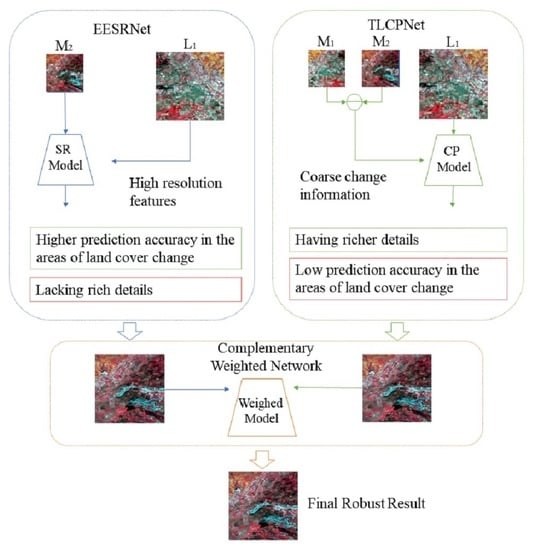
2.1. Method Overview

The flowchart of the proposed fusion method is shown in Figure 2. The first stage is the prediction stage via the dual-branch network, which consists of an edge-enhanced SR network (EESRNet) with a reference image and a two-layer change prediction network (TLCPNet) based on the attention mechanism [25]. The second stage is the weighting stage. The weighted network (WNet) is designed, and the final fusion result is obtained by weighing the two branches.

EESRNet transfers the coarse image into the fine image and eliminates the ambiguity and artifacts as much as possible through a series of optimization methods. The prediction image can be described as:

$$\begin{array}{c}\hfill L_2^{SR}(x_i,y_i,b)=SR(F\left(M_2(x_i,y_i,b)\right),F\left(L_1(x_i,y_i,b)\right),F(L_1\_R(x_i,y_i,b)))\end{array}$$

(1)

$M_1$ and $M_2$ refer to the coarse images at the reference date $t_1$ and the prediction date $t_2$. $L_1$ refers to the fine image at $t_1$ and $L_1\_R$ refers to the resample image of $L_1$. $SR$ refers to the SR model. F refers to feature extraction operation. $(x_i,y_i,b)$ stands for coordinates and bands respectively.

TLCPNet is composed of two networks with the same structure. According to the reference image and the change features from the coarse image sequence, the fine image at the prediction date is reconstructed. The prediction image can be described as:

$$\begin{array}{c}\hfill L_2^{CP}(x_i,y_i,b)=Re(F\left(L_1(x_i,y_i,b)\right)+F\left(M_2(x_i,y_i,b)\right)-F\left(M_1(x_i,y_i,b)\right))\end{array}$$

(2)

$Re$ refers to the image reconstruction model.

TLCPNet can predict rich spatial details based on the reference fine image but may introduce wrong details in the changing area. Therefore, TLCPNet shows better performance in phenological change and no-change areas, but poor performance in type change areas. EESRNet incorporates the phenological change, type changes, and no change in a unified fusion framework, and it has the same excellent performance in the three areas. However, compared to TLCPNet, the image details predicted by EESRNet are not rich enough due to the large magnification factor. The advantages of TLCPNet and EESRNet are complemented by weighting to improve the fusion results.

2.2. Edge-Enhanced Remote Sensing Super-Resolution Network with Reference Image

Compared with the SR of natural images (usually ranging from 2 to 4), the magnification factor of STF is much larger (usually ranging from 8 to 16). In that case, details have been severely blurred and distorted in coarse images. Remote sensing images contain more complex heterogeneous areas with abundant details, which further increase the difficulty in fine image prediction. Hence, it is impossible to accurately predict the fine image only by a coarse image. The fine image at the reference date is introduced to provide high-quality features for image SR. We propose an edge-enhanced super-resolution network with the reference image (EESRNet).

As shown in Figure 3, EESRNet is composed of three parts: a low-resolution feature (LF) extractor, high-resolution feature (HF) extractor, and image reconstruction module (IRM). LFs are extracted from the MODIS image and downsampled Landsat image by the LF extractor, as well as their edge maps. HFs are extracted from a Landsat image and its edge map by the HF extractor. The IRM uses these features to obtain the preliminary prediction result.

First, to make better use of the edge information, the image and the edge map of the image are used as the input to the feature extractor. The edge maps are obtained by Laplacian operator. The edge information is more conducive to image detail reconstruction, especially for the remote sensing image SR [26]. LF combines the features extracted from the low-resolution image and its edge maps. We call the edge combination feature(s) (ECF):

$$ECF(I,I\_edge)=F\left(I(x_i,y_i,b)\right)+F(I\_edge(x_i,y_i,b))$$

(3)

I and $I\_edge$ refer to the image and its edge map, respectively. The edge map feature can guide the construction of the image details and improve the performance of the image SR.

Figure 3. Architecture of the EESRNet. $M_2\_Edge$, $L_1\_Edge$, and $L_1\_R\_Edge$ refer to the edge map derived from the corresponding image, respectively. LF and HF refer to low-resolution features and high-resolution features, respectively.

Figure 3. Architecture of the EESRNet. $M_2\_Edge$, $L_1\_Edge$, and $L_1\_R\_Edge$ refer to the edge map derived from the corresponding image, respectively. LF and HF refer to low-resolution features and high-resolution features, respectively.

Second, LF from the MODIS image and downsampled Landsat image are concatenated to the reconstructed fine image at the prediction date. Since the coarse and fine images come from different sensors, the SR model also implies the sensor mapping relationship, which not only increases the complexity of the model but also reduces its robustness. To eliminate the influence of sensor differences, STFDCNN adds a non-linear mapping to transform the coarse image into a downsampled fine image, which is described as follows:

$$F\left(Modis\right)\Rightarrow F(Landsat\_LR)\Rightarrow F(Landsat\_HR)$$

(4)

However, the nonlinear mapping increases the computational cost and complexity of the STF algorithm. Therefore, we convert it in a more convenient way:

$$F\left(Modis\right)\cup F(Landsat\_LR)\Rightarrow F(Landsat\_HR)$$

(5)

Finally, IRM obtains preliminary prediction results by combining LFs and HFs. Due to the serious degradation of the coarse image, the fine image at the reference date is utilized to extract HFs. HFs can help to eliminate the noise interference of MODIS. Furthermore, the shallow and deep features of the HF extractor are introduced into the corresponding shallow and deep layers of the IRM to better reconstruct high-resolution images at the prediction date.

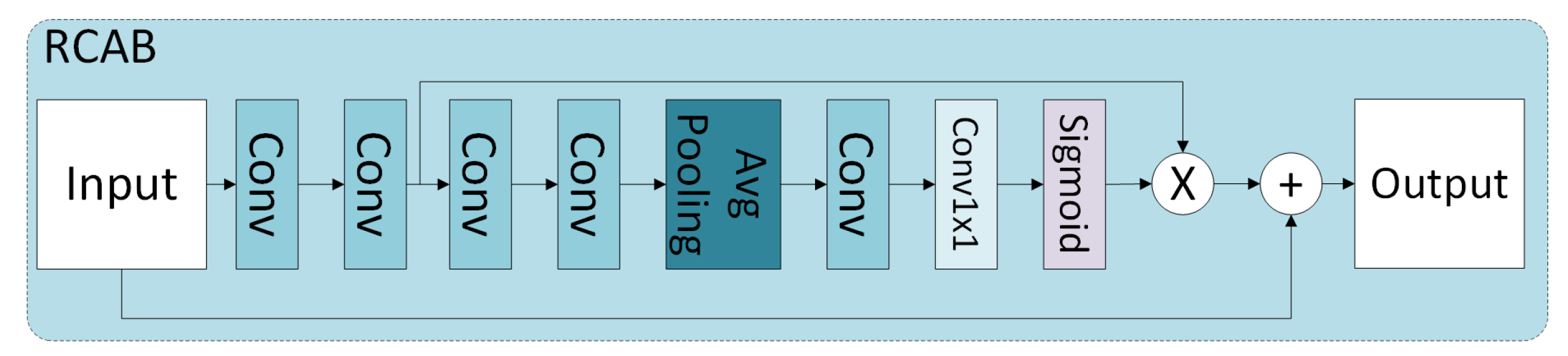
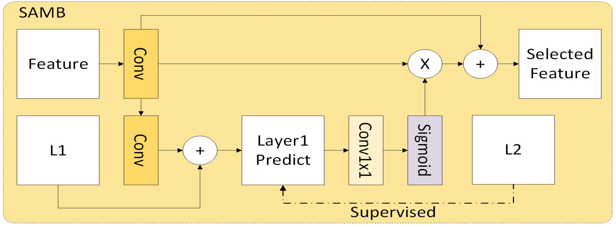
2.3. Two-Layer Change Prediction Network Based on Attention Mechanisms

The fine image prediction based on CP can be described by Equation (2) in Section 2.1. Due to insufficient datasets and seriously degraded coarse images, it is difficult to obtain accurate reconstruction models. To this end, we decompose the complex problem into two layers of the network. In this way, the complexity of each layer is reduced, the accuracy is improved, and the complex problem is solved step by step.

A two-layer change prediction network (TLCPNet) based on attention mechanisms is proposed. As shown in Figure 4, the two layers have the same structure, and there is a supervised attention mechanism block (SAMB) [27] between the two layers. The inputs of TLCPNet are coarse image sequences and a fine image at the reference date. In the training process, the two layers have their respective supervision.

As shown in Figure 4, the single-layer network consists of two separate convolutional layers, residual feature extractor (RFE), residual channel attention block (RCAB) [28], and UNet [29]. Two separate convolutional layers are responsible for converting backbone information and change information into corresponding feature information. RFE consisting of a four-layer convolutional residual network provides residual information to the network.

Figure 4. Architecture of the TLCPNet.

Figure 4. Architecture of the TLCPNet.

The RCAB is responsible for combining the backbone and change features, and filtering them on the channel level. As shown in Figure 5, RCAB consists of a global residual network. The RCAB makes the network pay attention to the relationship between different features at the channel level and assigns corresponding weights to each channel to strengthen features useful for image reconstruction.

The UNet, whose architecture is as shown in Figure 6, performs deeper feature extraction on the obtained shallow features and combines the features from RFE and RCAB. Our UNet can keep shallow features and deep features of backbone information and change information, which can improve the prediction performance.

The first layer network ($Laye{r}_1$) generates a rough prediction result using the features obtained by UNet through SAMB. We describe the whole process in $Laye{r}_1$ as:

$$\begin{array}{cc}\hfill P(x_i,y_i,b)=& R{e}_{Laye{r}_1}(F\left(L_1(x_i,y_i,b)\right)+F(M_2(x_i,y_i,b)-M_1(x_i,y_i,b))+\hfill \\ \hfill & RFE(L_1(x_i,y_i,b),M_1(x_i,y_i,b),M_2(x_i,y_i,b)))\hfill \end{array}$$

(6)

$P(x_i,y_i,b)$ refers to the prediction result of $Laye{r}_1$. Thus, the second layer network has a better reconstruction starting point. The second layer network ($Laye{r}_2$) completes the reconstruction task through a single convolution. We consider a similar process in $Laye{r}_2$:

$$L_2^{CP}(x_i,y_i,b)=R{e}_{Laye{r}_2}(F\left(P(x_i,y_i,b)\right)+RFE\left(P(x_i,y_i,b)\right)+SF)$$

(7)

$SF$ refers to the selected feature. The SAMB is used to select better reconstruction features from $Laye{r}_1$ for $Laye{r}_2$. As shown in Figure 7, we use a form of spatial attention for the feature selection task. Based on the above reasons, the final prediction result is improved.

2.4. Weighted Network

The weighted network is designed to integrate the complementary advantages of EESRNet and TLCPNet to improve the fusion results. The most commonly used weighting scheme is the weight function based on sliding window (WFSW), whose main characteristics are the fixed window size and fixed weight function. Take HDLSFM as an example; the weight is inversely proportional to the distance from the coarse image at the predicted date in a 3 × 3 sliding window. Due to the serious degradation of the coarse image, the distance from the coarse image cannot be equivalent to the degree far from the ideal value. In addition, due to the difference in the degradation degree in different areas (the detail-rich areas are more degraded than the flat areas), the fixed function cannot be adapted to all scenarios. Although various WFSW algorithms have been proved as statistically valid, the weight model based on deep learning can give a more accurate representation of complex scenes. Therefore, we designed a weighted network (WNet) as shown in Figure 8. Weight models that can represent various complex situations can be generated through deep learning. Moreover, in the form of a WNet, the two stages can be turned into a whole to participate in the training, which can better utilize the complementarity of the two branches. The weight calculation process of the two branches can be described as:

$$WeightMap(x_i,y_i,b)=sub\_WNet\left(I(x_i,y_i,b)\right)$$

(8)

The $sub\_WNet$ refers to the sub-branch of the WNet. $I(x_i,y_i,b)$ refers to the input of the sub-branch. As shown in Figure 8, we use several layers of residual networks to build the network. Our final prediction is the dot product sum of the branch prediction and its weight map.

$$Final\_Result=w_1*Result\_SR+w_2*Result\_CP$$

(9)

$w_1$ refers to the weight map of the EESRNet result. $w_2$ refers to the weight map of the TLCPNet result. $Result\_SR$ refers to the preliminary prediction result of the EESRNet. $Result\_CP$ refers to the preliminary prediction result of the TLCPNet.

Figure 8. Architecture of the WNet.

Figure 8. Architecture of the WNet.

2.5. Loss Function

In the training phase, our algorithm needs to calculate the output loss of two branches and the output loss of the whole network, respectively. These loss functions adopt the same expression. Our loss function consists of content loss, feature loss, and structure loss, formulated as Equation (10),

$$Loss=Loss\_feature+Loss\_content+Loss\_structure$$

(10)

To calculate the feature loss, the most usual feature extractors in natural image tasks are from the VGG network pre-trained on ImageNet. However, the feature distribution of a remote sensing image is obviously different from that of a natural image. We pre-trained an encode–decode network (EDNet) [16] for better feature representation and feature loss calculation. The feature loss and content loss are calculated by the mean square error (MSE) and defined as:

$$Loss\_feature=MSE(EDNet\left(L_2\right),EDNet\left(Prediction\right))$$

(11)

$$Loss\_content=MSE(L_2,Prediction)$$

(12)

We evaluate structural losses using the multi-scale structural similarity index (mssim) [30]. The structural loss is defined as:

$$Loss\_structure=1-mssim(L_2,Prediction)$$

(13)

3. Experiment

3.1. Experiment Datasets

To better verify the universality of our algorithm for various scenarios, the following three types of scene images from Landsat-MODIS datasets were selected in our experiments: (1) type change, (2) phenological change, and (3) heterogeneous landscape. The following are the experimental dataset descriptions.

The lower Gwydir catchment (LGC) is located in northern New South Wales, Australia. The LGC dataset includes significant land cover type changes due to the occurrence of a large flood. The dataset is used to test the generalization ability of our algorithm and the ability to predict type changes. Figure 9 shows the test data we used on the LGC dataset.

The Ar Horqin banner (AHB) is located in Inner Mongolia Province, China. The main industry of AHB is agriculture and animal husbandry, with a large number of circular pastures and farmland. The time span of the AHB dataset is more than 5 years, and there are significant phenological changes with the response of time and season to climate change. Because of the obvious error of the MODIS short-wave infrared band on this dataset [31], only four bands were used in the experiment. Figure 10 shows the test data we used on the AHB dataset.

The Coleambally irrigation area (CIA) is located in southern New South Wales, Australia. The CIA dataset contains a large number of irregularly shaped irrigated farmlands, and the sizes of farmlands are relatively small. Thus, we can consider CIA a spatially heterogeneous area with multiple phenological changes. Figure 11 shows the test data we used on the CIA dataset.

Figure 9. Test data from the LGC dataset. These figures exhibit the false color composite images using band 4, band 3, and band 2. (a,c) are the MOIDS and Landsat images on 26 November 2004, respectively. (b,d) are the MOIDS and Landsat images on 12 December 2004, respectively.

Figure 9. Test data from the LGC dataset. These figures exhibit the false color composite images using band 4, band 3, and band 2. (a,c) are the MOIDS and Landsat images on 26 November 2004, respectively. (b,d) are the MOIDS and Landsat images on 12 December 2004, respectively.

Figure 10. Test data from the AHB dataset. These figures exhibit the false color composite images using band 4, band 3, and band 2. (a,c) are the MOIDS and Landsat images on 29 August 2017, respectively. (b,d) are the MOIDS and Landsat images on 4 January 2018, respectively.

Figure 10. Test data from the AHB dataset. These figures exhibit the false color composite images using band 4, band 3, and band 2. (a,c) are the MOIDS and Landsat images on 29 August 2017, respectively. (b,d) are the MOIDS and Landsat images on 4 January 2018, respectively.

Figure 11. Test data from the CIA dataset. These figures exhibit the false color composite images using band 4, band 3, and band 2. (a,c) are the MOIDS and Landsat images on 11 January 2002, respectively. (b,d) are the MOIDS and Landsat images on 12 February 2002, respectively.

Figure 11. Test data from the CIA dataset. These figures exhibit the false color composite images using band 4, band 3, and band 2. (a,c) are the MOIDS and Landsat images on 11 January 2002, respectively. (b,d) are the MOIDS and Landsat images on 12 February 2002, respectively.

3.2. Experiment Design and Evaluation

Two traditional STF methods (STARFM, FSDAF) and three deep learning-based methods(STFDCNN, EDCSTFN, HDLSFM) are used for comparison. We used PyTorch to build our experimental code to complete the experiments on Intel 10,700 k and Nvidia RTX 3090. For the different dataset experiments, we used different patch sizes. For LGC and AHB, we cropped the image size to 2400 × 2400 and used a patch size of 240 × 240. For CIA, we cropped the image size to 1280 × 1280 and used a patch size of 160 × 160. The overlapping patch training scheme was not used, and the stride size was set to the same as the corresponding patch size. The batch size was set to 16. The epoch was set to 90 for each group of experiments. We used Adam [32] as the optimization algorithm, the learning rate was $5\times {10}^4$, the weight decay was $1\times {10}^{-6}$, and other hyperparameters were the default values.

In order to evaluate the experimental results objectively and comprehensively, we selected six representative evaluation indexes from the aspects of spatial and spectral quality. These indexes are root mean square error (RMSE), structure similarity (SSIM) [33], correlation coefficient (CC), peak-signal-to-noise ratio (PSNR), erreur relative global adimensionnelle de synthese (ERGAS) [34], and spectral angle mapper (SAM) [35]. Among them, SSIM is a spatial quality index, SAM is a spectral quality index, and RMSE, ERGAS, and CC are spatial–spectral quality indexes. RMSE, expressed by Equation (14), was used to gauge the difference between the predicted reflectance and the actual reflectance.

$$RMSE=\sqrt{\frac{{\sum }_{i=1}^N{(y_i-{\widehat{y}}_i)}^2}{N}}$$

(14)

N denotes the total number of pixels of the image; $y_i$ and ${\widehat{y}}_i$ denote the ith observed value and predicted value. SSIM, expressed by Equation (15), was also used to evaluate the similarity of the overall structure between the true and predicted images.

$$SSIM=\frac{(2{\mu }_x{\mu }_y+C_1)(2{\sigma }_{xy}+C_2)}{({\mu }_x^2+{\mu }_y^2+C_1)({\sigma }_x+{\sigma }_y+C_2)}$$

(15)

${\mu }_x$ and ${\mu }_y$ are means, ${\sigma }_x$ and ${\sigma }_y$ are the variances of the true and predicted images, ${\sigma }_{xy}$ is the covariance of the two images, $C_1$ and $C_2$ are the two small constants used to avoid unstable results when the denominator of Equation (16) is very close to zero. CC, expressed by Equation (17), was used to show the linear relationship between predicted and actual reflectance.

$$CC=\frac{{\sum }_{i=1}^N{y}_i{\widehat{y}}_i}{\sqrt{{\sum }_{i=1}^N{y}_i^2}\sqrt{{\sum }_{i=1}^N{\widehat{y}}_i^2}}$$

(16)

PSNR, expressed by Equation (14), was used to measure the quality of predicted images.

$$PSNR=10·lo{g}_{10}\left(\frac{MA{X}_I^2}{MSE}\right)$$

(17)

$MA{X}_I$ refers to the maximum pixel value of the corresponding bit image. $MSE$ refers to mean square error. ERGAS, expressed by Equation (18), was used to show the overall performance of the image.

$$ERGAS=100\frac{h}{l}\sqrt{\frac{1}{M}{\sum }_{i=1}^M[RMSE{\left(L_i\right)}^2/{\left({\mu }_i\right)}^2]}$$

(18)

h and l refer to the resolution of the high-resolution image and fine-resolution image, respectively. M refers to the band of images. $L_i$ refers to the ith band image and ${\mu }_i$ refers to its mean value. SAM, expressed by Equation (19), was used to evaluate the spectral performance of the predict.

$$SAM=\frac{1}{N}\sum _{i=1}^{N}arccos\frac{{\sum }_{j=1}^M{L}_i^j{\widehat{L}}_i^j}{\sqrt{{\sum }_{j=1}^M{\left(L_i^j\right)}^2{\sum }_{j=1}^M{\left({\widehat{L}}_i^j\right)}^2}}$$

(19)

3.3. Experiment Results

3.3.1. Experiment A: Exploring the Performance of Algorithm in Type Change

Figure 12 shows the fusion results of our method and contrastive algorithm on the LGC dataset and the ground truth as the evaluation. We first evaluated our experimental results on intuitive visual performance. The DL-based algorithms have better performance than the traditional algorithms, and the overall performance of our algorithm is better than other DL-based algorithms. STARFM has serious distortion in the shape and color of the image. FSDAF results in the outer edge of the water being blurred. STFDCNN still has a certain block effect. The prediction results of HDLSFM are not sufficient in terms of spectrum and deformation. The bluer the average difference map is, the closer the result is to the ground truth. Obviously, our difference map is the bluest. From the comparison of the average surface reflection change map, it can also be seen that our algorithm and EDCSTFN are closer to the real situation in the prediction of the change areas. However, our method performs better in the changing areas in the lower left corner. In summary, our method exhibits richer details with other comparative methods under complex type changes.

According to the quantitative evaluation shown in

Table 1. Evaluation metrics of LGC prediction results. Bold values indicate the best results.

	Band	STARFM	FSDAF	STFDCNN	EDCSTFN	HDLSFM	Ours
RMSE	band1	0.0671	0.0608	0.0577	0.0575	0.0709	0.0495
	band2	0.0915	0.0829	0.0803	0.0801	0.1063	0.0701
	band3	0.1121	0.1018	0.0989	0.1013	0.1306	0.0869
	band4	0.1638	0.1615	0.1346	0.1509	0.1634	0.1423
	band5	0.2727	0.2738	0.2180	0.2308	0.2633	0.2206
	band7	0.2380	0.2396	0.1703	0.1727	0.1983	0.1636
	avg	0.1576	0.1534	0.1266	0.1322	0.1555	0.1222
SSIM	band1	0.6980	0.7218	0.7399	0.7661	0.7028	0.7934
	band2	0.6808	0.7115	0.7283	0.7485	0.6712	0.7831
	band3	0.6861	0.7116	0.7422	0.7459	0.6780	0.7888
	band4	0.7933	0.8007	0.8510	0.8219	0.7922	0.8267
	band5	0.7465	0.7388	0.8161	0.8264	0.7740	0.8246
	band7	0.6756	0.6600	0.7995	0.8176	0.7680	0.8319
	avg	0.7134	0.7241	0.7795	0.7877	0.7310	0.8081
CC	band1	0.7002	0.7250	0.7416	0.7830	0.7130	0.8059
	band2	0.6813	0.7174	0.7345	0.7703	0.6839	0.7993
	band3	0.6863	0.7186	0.7446	0.7644	0.6921	0.8014
	band4	0.8059	0.8276	0.8614	0.8329	0.7996	0.8484
	band5	0.7704	0.7764	0.8247	0.8322	0.7847	0.8368
	band7	0.7390	0.7438	0.8053	0.8255	0.7819	0.8432
	avg	0.7305	0.7515	0.7853	0.8014	0.7425	0.8225
PSNR	band1	50.8121	51.4574	51.7529	51.6421	50.3942	52.7013
	band2	48.6171	49.3067	49.5108	49.4070	47.5024	50.3989
	band3	47.0945	47.8015	48.0375	47.8118	45.9352	48.9266
	band4	44.1177	44.2285	45.6888	44.7855	44.1405	45.2478
	band5	39.8971	39.8665	41.7810	41.3061	40.1913	41.6843
	band7	41.0475	40.9871	43.8792	43.7893	42.5744	44.2330
	avg	45.2643	45.6079	46.7750	46.4570	45.1230	47.1987
ERGAS		4.0797	4.0170	3.4131	3.2708	3.8665	3.1786
SAM		13.8487	12.9682	8.9418	9.1865	12.1420	8.8463

, firstly, our method shows minimal RMSE. Compared with the suboptimal STFDCNN, RMSE is reduced by 3.476%. Secondly, the average quantization indices of SSIM, PSNR, and CC show that our algorithm does improve the fusion accuracy. Compared with the suboptimal index, SSIM, CC, and PSNR increase by 2.577%, 2.633%, and 0.906%, respectively. Finally, our algorithm decreases by 1.068% in SAM and 2.819% in ERGAS compared with the suboptimal STFDCNN. RMSE, ERGAS, PSNR, and CC reflect that the overall performance of our algorithm is excellent, and the fusion result is closer to the ground truth. The highest SSIM and SAM indicate that our results have significant advantages in terms of spatial structure and spectral fidelity. These quantitative results demonstrate that WDBSTF can better adapt to type change.

Figure 12. The fusion results on 12 December 2001 in LGC (the first row exhibits the false color composite images using band 4, band 3, and band 2; the second row exhibits the zoomed-in details of the yellow rectangles marked in the first row; the third row exhibits the average difference map between the prediction and ground truth; the fourth row exhibits the average surface reflection change map).

Figure 12. The fusion results on 12 December 2001 in LGC (the first row exhibits the false color composite images using band 4, band 3, and band 2; the second row exhibits the zoomed-in details of the yellow rectangles marked in the first row; the third row exhibits the average difference map between the prediction and ground truth; the fourth row exhibits the average surface reflection change map).

3.3.2. Experiment B: Exploring the Performances of Algorithms in Phenological Changes

Figure 13 shows the fusion results of our algorithm and the comparison algorithm on the AHB dataset and ground truth as the evaluation. From an intuitive evaluation, our algorithm is closer to ground truth in terms of overall color and texture style. There are drastic color changes between the reference date and prediction date. Both STARFM and FSDAF show obvious chromatic aberration and halo phenomenon. We can see that there is a relatively obvious motion blur [36] on the MODIS image. This is mainly because the relative motion between the acquisition device and target occurs at the instance image exposure of the image acquisition, resulting in the offset and superposition of the beam. Neither STFDCNN nor HDLSFM can effectively remove motion blur. Instead, they amplify the motion blur feature, which results in oblique stripes in the final prediction. Our average difference map is the bluest and the average surface reflection change map is also closer to the real situation. Although both the EDCSTFN and our eliminate the effect of motion blur, compared to the EDCSTFN, our algorithm is richer in color representation. To sum up, our algorithm has a more robust performance in handling drastic phenological changes and eliminating motion blur.

Table 2. Evaluation metrics of AHB prediction results. Bold values indicate the best results.

	Band	STARFM	FSDAF	STFDCNN	EDCSTFN	HDLSFM	Ours
RMSE	band1	0.1223	0.1219	0.0200	0.0137	0.0237	0.0081
	band2	0.1061	0.1058	0.0168	0.0139	0.0195	0.0099
	band3	0.1429	0.1415	0.0244	0.0168	0.0263	0.0140
	band4	0.1337	0.1307	0.0348	0.0326	0.0365	0.0244
	avg	0.1263	0.1250	0.0240	0.0193	0.0265	0.0141
SSIM	band1	0.5747	0.5705	0.8878	0.9266	0.8097	0.9644
	band2	0.6867	0.6848	0.9519	0.9550	0.9241	0.9712
	band3	0.6446	0.6454	0.9435	0.9660	0.9131	0.9698
	band4	0.7845	0.7897	0.9469	0.9530	0.9019	0.9590
	avg	0.6726	0.6726	0.9325	0.9501	0.8872	0.9661
CC	band1	0.4368	0.6668	0.5658	0.6148	0.5228	0.7177
	band2	0.6289	0.6953	0.6571	0.7176	0.5659	0.7598
	band3	0.6023	0.6512	0.5955	0.7252	0.4847	0.7401
	band4	0.5864	0.6162	0.5278	0.6844	0.4448	0.6975
	avg	0.5636	0.6574	0.5865	0.6855	0.5045	0.7288
PSNR	band1	18.2502	18.2795	33.9727	37.2373	32.4955	41.8343
	band2	19.4867	19.5102	35.4971	37.1236	34.2032	40.0772
	band3	16.9014	16.9856	32.2522	35.5138	31.5848	37.0757
	band4	17.4744	17.6777	29.1667	29.7241	28.7553	32.2565
	avg	18.0282	18.1132	32.7222	34.8997	31.7597	37.8109
ERGAS		5.3351	5.3112	3.8448	3.5259	3.9795	3.1030
SAM		20.4020	20.3929	7.6826	3.9386	11.1393	2.7584

shows the specific quantitative evaluation metrics of Experiment B. Our methods achieve the best on all metrics. Our algorithm outperforms the corresponding suboptimal algorithms by 26.94%, 1.684%, 6.317%, 8.342%, 29.96%, and 11.23% on RMSE, SSIM, CC, PSNR, SAM, and ERGAS, respectively. These quantitative results demonstrate that WDBSTF can be well adapted to scenes with phenological changes and motion blur. Moreover, The quantitative metrics of STFDCNN and HDLSFM also show that the inability to eliminate motion blur has a serious impact on the results.

Figure 13. The fusion results on 4 January 2018 in AHB (the arrangement of the subfigures is the same as the above).

Figure 13. The fusion results on 4 January 2018 in AHB (the arrangement of the subfigures is the same as the above).

3.3.3. Experiment C: Exploring the Performance of the Algorithm in a Heterogeneous Landscape

Figure 14 shows the fusion results of our method and comparison algorithm on the CIA dataset and the ground truth as the evaluation. The main changes in the data are the differences in vegetation growth and the surface reflection of the irrigation water body. From the intuitive evaluation, there is little difference between the prediction results of different methods. From the overall color style of the zoomed-in local area, STFDCNN and our algorithm are the closest to ground truth. STARFM, FSDAF, and HDLSFM exhibited whiter colors, while EDCSTFN exhibited darker greens. From the comparison with STFDCNN, our average difference map is bluer and the average surface reflection change map is also closer to the real situation. In summary, our method exhibits more robust performance than other comparative methods in a heterogeneous landscape area.

Table 3. Evaluation metrics of CIA prediction results. Bold values indicate the best results.

	Band	STARFM	FSDAF	STFDCNN	EDCSTFN	HDLSFM	Ours
RMSE	band1	0.1024	0.0889	0.0757	0.0799	0.0951	0.0692
	band2	0.1632	0.1326	0.1038	0.1109	0.1412	0.0974
	band3	0.2717	0.2079	0.1600	0.2075	0.2276	0.1405
	band4	0.4716	0.3971	0.2754	0.3417	0.4176	0.2862
	band5	0.3340	0.2807	0.2659	0.2739	0.3055	0.2625
	band7	0.2662	0.2336	0.2312	0.2364	0.2443	0.2327
	avg	0.2682	0.2235	0.1853	0.2084	0.2385	0.1814
SSIM	band1	0.8740	0.9005	0.9264	0.8997	0.8898	0.9278
	band2	0.8367	0.8823	0.9190	0.8878	0.8662	0.9169
	band3	0.8337	0.8906	0.9261	0.9080	0.8699	0.9365
	band4	0.5863	0.6618	0.8574	0.8023	0.6250	0.8567
	band5	0.9062	0.9311	0.9371	0.9241	0.9205	0.9357
	band7	0.9269	0.9416	0.9431	0.9344	0.9375	0.9384
	avg	0.8273	0.8680	0.9182	0.8927	0.8515	0.9187
CC	band1	0.8816	0.9045	0.9278	0.9108	0.8929	0.9352
	band2	0.8517	0.8889	0.9194	0.9056	0.8720	0.9266
	band3	0.8557	0.8993	0.9264	0.9163	0.8803	0.9402
	band4	0.5865	0.6716	0.8591	0.8032	0.6351	0.8572
	band5	0.9075	0.9312	0.9372	0.9332	0.9211	0.9443
	band7	0.9272	0.9416	0.9432	0.9409	0.9377	0.9464
	avg	0.8350	0.8729	0.9189	0.9017	0.8565	0.9250
PSNR	band1	52.0626	52.8371	53.8265	53.2995	52.1282	53.7872
	band2	48.9261	50.2918	52.0281	51.7482	49.8488	52.4045
	band3	45.1920	47.2700	49.0842	47.1689	46.5798	49.8942
	band4	40.6068	42.0486	45.0620	43.2943	41.6327	44.7219
	band5	43.4576	44.8760	45.3143	45.0985	44.1878	45.4340
	band7	45.2783	46.2860	46.3466	46.0842	45.9509	46.2221
	avg	45.9206	47.2682	48.6103	47.7823	46.7214	48.7440
ERGAS		2.9060	2.6700	2.3985	2.5402	2.8036	2.3886
SAM		5.8321	4.8365	3.9851	4.7364	5.4252	3.7658

shows the specific quantitative evaluation metrics of Experiment C. The better performance of the indicators is mainly reflected in our algorithm and STFDCNN. Our algorithm achieves the best performance on average, and outperforms the suboptimal algorithms by 2.105%, 0.0545%, 0.664%, 0.275%, 5.55%, and 0.413% on RMSE, SSIM, CC, PSNR, SAM, and ERGAS, respectively. These quantitative results demonstrate that WDBSTF can be well adapted to a scene with a heterogeneous landscape.

4. Discussion

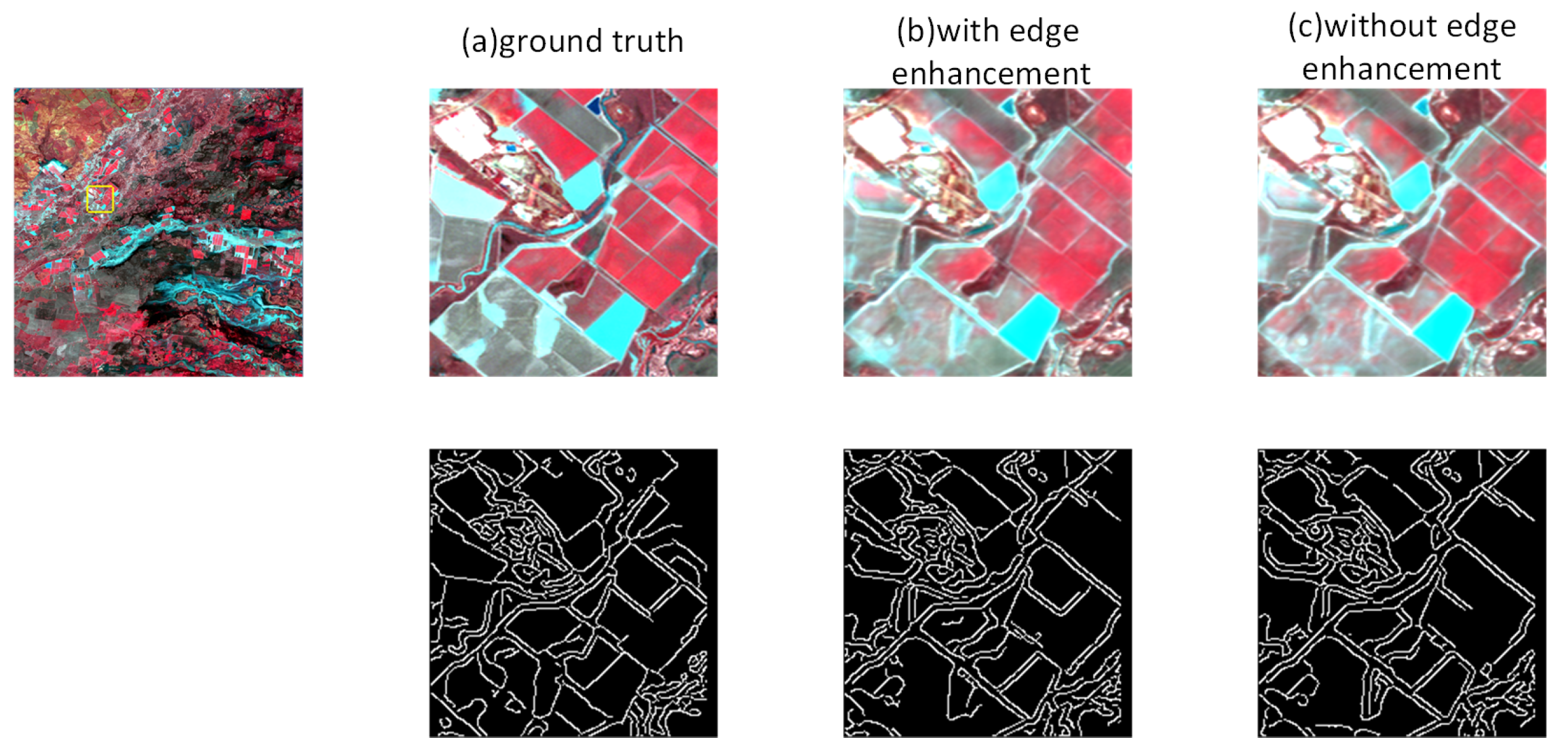
4.1. Exploring the Influence of Edge Enhancement on Prediction Results

To verify the effect of edge enhancement on the results, we performed experiments on the three datasets after removing and retaining the input edge extraction features separately.

Table 4. Evaluation metrics on the results of ablation experiments of edge enhancement on different datasets. Bold values indicate the best results.

	With Edge Enhancement			Without Edge Enhancement
	LGC	AHB	CIA	LGC	AHB	CIA
RMSE	0.1222	0.0141	0.1814	0.1275	0.0169	0.1986
SSIM	0.8081	0.9661	0.9187	0.7972	0.9580	0.8995
CC	0.8225	0.7288	0.9250	0.8133	0.6751	0.9055
PSNR	47.1987	37.8109	48.7440	46.8941	36.6753	48.1105
ERGAS	3.1786	3.1030	2.3886	3.2134	3.2536	2.4739
SAM	8.8463	2.7584	3.7658	9.1642	3.1826	4.3976

shows our experimental results. It can be seen that the final results are optimized by the edge enhancement of ECF.

In order to present our results more intuitively, we selected an area of the predicted results from the LGC dataset for display. Moreover, we show the edge extraction maps corresponding to each result, and the edge extraction maps are obtained by the Canny algorithm [37]. Figure 15 shows the results of related experiments on the LGC dataset. From a direct observation, the difference between the results with and without edge enhancement operation is not obvious. However, it can be seen from the edge maps that the results with ECF added are closer to the ground truth in terms of edges. For results without ECF, more false edges are generated. This leads to a worse structural performance of the final result. The analysis of quantitative metrics for the three datasets shows that ECF has a better advantage in edge-guided structure generation.

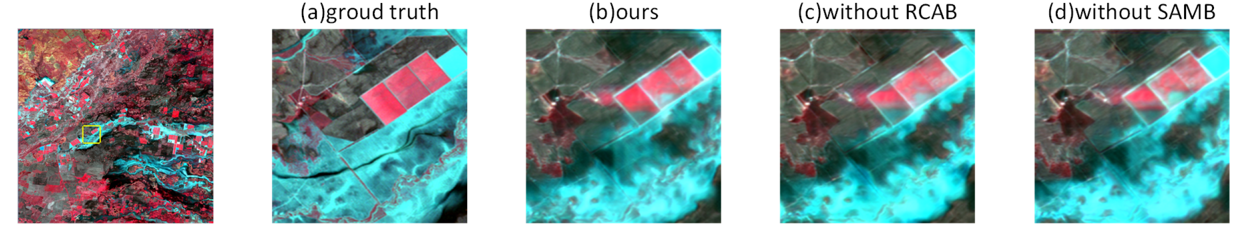
4.2. Exploring the Influence of Attention Mechanism on Prediction Results

We use the channel-based attention mechanism RCAB and the spatial-based attention mechanism SAMB in TLCPNet. To verify the effectiveness of the two modules on the results, we tested the experimental results on three datasets after removing the two modules, respectively. Figure 16 shows the experimental results of removing the two modules on the LGC dataset, and we can see that the prediction of the middle water part of the image is not as good as the original result after removing both modules, respectively.

Table 5. Evaluation metrics on the results of ablation experiments of attention mechanism on different datasets. Bold values indicate the best results.

	With Attention Mechanism			Without RCAB			Without SAMB
	LGC	AHB	CIA	LGC	AHB	CIA	LGC	AHB	CIA
RMSE	0.1222	0.0141	0.1814	0.1238	0.0170	0.1989	0.1245	0.0197	0.2080
SSIM	0.8081	0.9661	0.9187	0.8047	0.9532	0.8907	0.8018	0.9360	0.8997
CC	0.8225	0.7288	0.9250	0.8179	0.6951	0.9019	0.8150	0.6884	0.9066
PSNR	47.1987	37.8109	48.7440	47.1112	36.1273	48.0364	47.0286	34.5176	47.7171
ERGAS	3.1786	3.1030	2.3886	3.2001	3.3196	2.4484	3.2071	3.5358	2.4360
SAM	8.8463	2.7584	3.7658	8.8418	2.9602	4.3116	8.9166	2.8246	4.2420

shows the quantitative evaluation metrics of the corresponding experiments. By comparing the specific quantitative results, we can see that the experimental results after removing the two modules are worse than those after retaining them on all three datasets, indicating that the two are positively boosted for our prediction process. We can effectively improve the metrics of the prediction results by enhancing the attention of the features in the channel dimension and the spatial dimension. The experimental results of removing SAMB also illustrate the positive effect of selecting features valuable for image reconstruction on the results.

4.3. Comparison with Other STF Algorithms

Traditional algorithms, such as STARFM and FSDAF, can usually produce relatively stable results. However, the results on the three datasets also show that the two methods cannot produce sufficiently robust results in the case of complex cover changes. This may be because both use a linear relationship to obtain the final prediction. The performance of linear relationships for complex scene changes is limited. DL-based algorithms can often achieve better performance than traditional algorithms. The results on the CIA datasets show that STFDCNN achieves better performance on phenological changes because of two references. However, in the large type change areas of LGC, STFDCNN produces a severe block effect. This is because it adopts direct end-to-end mapping of coarse and fine images. For huge resolution differences, direct mapping may not be able to effectively generate high-quality images. Thus, STFDCNN uses high-pass modulation to enhance image quality. However, the use of high-pass modulation also introduces unnecessary features to the result. At the same time, direct mapping may not be able to remove noise effects in MODIS images. The results of the AHB dataset show the oblique stripes phenomenon. Due to the lack of valid high-resolution information, the motion blur is enhanced into diagonal stripes, which produces a large deviation from the ground truth. For HDLSFM, the double branch weighting enables the results to obtain better performance. However, LC with a similar structure to STFDCNN also produces results with oblique stripes on AHB datasets. EDCSTFN is a suboptimal method used for handling large change areas. The difference of MODIS can eliminate the influence of motion blur to a certain extent, so as to not produce oblique stripes. However, the change information provided by the MODIS difference is limited. We can see that EDCSTFN results still have considerable deviations in some details.

Our method achieves the best performance in all three scenarios. We summarize the reasons from four aspects: (1) We design a super-resolution model called EESRNet with high-resolution image references. EESRNet provides structured guidance for result generation via ECF. The combination of low-resolution image features from different satellites can ensure a similar function to the radiance normalization of different sensors in STFDCNN. HF can help to eliminate the noise interference of MODIS. EESRNet does not produce diagonal stripes due to motion blur. In summary, the network can generate higher-quality images without additional image enhancement operations. (2) We designed a TLCPNet for the CP task. The gradual restoration of the two-layer structure decomposes the original difficult problem into two easier sub-problems, thereby improving the overall network performance. The introduction of the attention mechanism can also improve the performance of the network. (3) Although EESRNet obtains higher-quality generation results, its details are still insufficient compared to the CP branch. Although the TLCPNet obtains a more stable performance, providing more reference information for the changing areas is undoubtedly more conducive to the accuracy of the results. Combining the CP branch to improve the details of the SR results and combining the SR branch to provide more change areas references for the CP results can make the results of the two branches promote each other and obtain more robust prediction results. So, we designed a WNet to generate the weight for two branch results. The training-based weights were obtained through nonlinear mapping, which can be applied to more complex changing scenarios, resulting in more robust results. (4) We added independent supervision to the generated results of EESRNet and TLCPNet. Overall supervision also promoted per-module and overall generated results closer to ground truth.

5. Conclusions

In this paper, we proposed a weighted and multi-supervised WDBSTF based on complementary SR and CP branch networks. Quantitative and visual evaluations of contrastive experiments demonstrate the superiority of WDBSTF. The advantages of our model are threefold: (1) Edge enhancement and high-resolution feature reference can enable SR models to obtain higher-quality images without additional image enhancement operations. (2) Decomposing the complex change prediction problem into sub-problems through a two-layer network can make the CP network have a more stable performance. (3) The trained weighted network can better combine the advantages of the two complementary branches for more robust final prediction results. However, our network still has difficulty in training due to a large number of parameters and the complex network structure. Our future work can consider more lightweight models to complete the work. At the same time, the vision transformer [38,39] has brought about a higher baseline to some image processing fields compared to CNN. Our future work will also consider the vision transformer as a backbone to develop more efficient networks.

References

1. Shi, C.; Wang, X.; Zhang, M.; Liang, X.; Niu, L.; Han, H.; Zhu, X. A comprehensive and automated fusion method: The enhanced flexible spatiotemporal data fusion model for monitoring dynamic changes of land surface. Appl. Sci. 2019, 9, 3693. [Google Scholar] [CrossRef] [Green Version]
2. Shen, Y.; Shen, G.; Zhai, H.; Yang, C.; Qi, K. A Gaussian Kernel-Based Spatiotemporal Fusion Model for Agricultural Remote Sensing Monitoring. IEEE J. Sel. Top. Appl. Earth Obs. Remote Sens. 2021, 14, 3533–3545. [Google Scholar] [CrossRef]
3. Li, P.; Ke, Y.; Wang, D.; Ji, H.; Chen, S.; Chen, M.; Lyu, M.; Zhou, D. Human impact on suspended particulate matter in the Yellow River Estuary, China: Evidence from remote sensing data fusion using an improved spatiotemporal fusion method. Sci. Total Environ. 2021, 750, 141612. [Google Scholar] [CrossRef] [PubMed]
4. Zhu, X.; Cai, F.; Tian, J.; Williams, T.K.A. Spatiotemporal fusion of multisource remote sensing data: Literature survey, taxonomy, principles, applications, and future directions. Remote Sens. 2018, 10, 527. [Google Scholar] [CrossRef] [Green Version]
5. Gao, F.; Masek, J.; Schwaller, M.; Hall, F. On the blending of the Landsat and MODIS surface reflectance: Predicting daily Landsat surface reflectance. IEEE Trans. Geosci. Remote Sens. 2006, 44, 2207–2218. [Google Scholar]
6. Hilker, T.; Wulder, M.A.; Coops, N.C.; Linke, J.; McDermid, G.; Masek, J.G.; Gao, F.; White, J.C. A new data fusion model for high spatial-and temporal-resolution mapping of forest disturbance based on Landsat and MODIS. Remote Sens. Environ. 2009, 113, 1613–1627. [Google Scholar] [CrossRef]
7. Zhu, X.; Chen, J.; Gao, F.; Chen, X.; Masek, J.G. An enhanced spatial and temporal adaptive reflectance fusion model for complex heterogeneous regions. Remote Sens. Environ. 2010, 114, 2610–2623. [Google Scholar] [CrossRef]
8. Zhu, X.; Helmer, E.H.; Gao, F.; Liu, D.; Chen, J.; Lefsky, M.A. A flexible spatiotemporal method for fusing satellite images with different resolutions. Remote Sens. Environ. 2016, 172, 165–177. [Google Scholar] [CrossRef]
9. Huang, B.; Song, H. Spatiotemporal reflectance fusion via sparse representation. IEEE Trans. Geosci. Remote Sens. 2012, 50, 3707–3716. [Google Scholar] [CrossRef]
10. Song, H.; Huang, B. Spatiotemporal satellite image fusion through one-pair image learning. IEEE Trans. Geosci. Remote Sens. 2012, 51, 1883–1896. [Google Scholar] [CrossRef]
11. Wu, B.; Huang, B.; Zhang, L. An error-bound-regularized sparse coding for spatiotemporal reflectance fusion. IEEE Trans. Geosci. Remote Sens. 2015, 53, 6791–6803. [Google Scholar] [CrossRef]
12. Wei, J.; Wang, L.; Liu, P.; Song, W. Spatiotemporal fusion of remote sensing images with structural sparsity and semi-coupled dictionary learning. Remote Sens. 2016, 9, 21. [Google Scholar] [CrossRef] [Green Version]
13. Song, H.; Liu, Q.; Wang, G.; Hang, R.; Huang, B. Spatiotemporal satellite image fusion using deep convolutional neural networks. IEEE J. Sel. Top. Appl. Earth Obs. Remote Sens. 2018, 11, 821–829. [Google Scholar] [CrossRef]
14. Tan, Z.; Di, L.; Zhang, M.; Guo, L.; Gao, M. An enhanced deep convolutional model for spatiotemporal image fusion. Remote Sens. 2019, 11, 2898. [Google Scholar] [CrossRef] [Green Version]
15. Jia, D.; Cheng, C.; Song, C.; Shen, S.; Ning, L.; Zhang, T. A hybrid deep learning-based spatiotemporal fusion method for combining satellite images with different resolutions. Remote Sens. 2021, 13, 645. [Google Scholar] [CrossRef]
16. Tan, Z.; Gao, M.; Li, X.; Jiang, L. A flexible reference-insensitive spatiotemporal fusion model for remote sensing images using conditional generative adversarial network. IEEE Trans. Geosci. Remote Sens. 2021, 60, 1–13. [Google Scholar] [CrossRef]
17. Song, Y.; Zhang, H.; Huang, H.; Zhang, L. Remote Sensing Image Spatiotemporal Fusion via a Generative Adversarial Network with One Prior Image Pair. IEEE Trans. Geosci. Remote Sens. 2022, 60, 1–17. [Google Scholar] [CrossRef]
18. Lei, D.; Ran, G.; Zhang, L.; Li, W. A Spatiotemporal Fusion Method Based on Multiscale Feature Extraction and Spatial Channel Attention Mechanism. Remote Sens. 2022, 14, 461. [Google Scholar] [CrossRef]
19. Dong, C.; Loy, C.C.; He, K.; Tang, X. Learning a deep convolutional network for image super-resolution. In Proceedings of the European Conference on Computer Vision, Zurich, Switzerland, 6–12 September 2014; Springer: Berlin/Heidelberg, Germany, 2014; pp. 184–199. [Google Scholar]
20. Ledig, C.; Theis, L.; Huszár, F.; Caballero, J.; Cunningham, A.; Acosta, A.; Aitken, A.; Tejani, A.; Totz, J.; Wang, Z.; et al. Photo-realistic single image super-resolution using a generative adversarial network. In Proceedings of the IEEE Conference on Computer Vision and Pattern Recognition, Honolulu, HI, USA, 21–26 July 2017; pp. 4681–4690. [Google Scholar]
21. Zhang, H.; Song, Y.; Han, C.; Zhang, L. Remote sensing image spatiotemporal fusion using a generative adversarial network. IEEE Trans. Geosci. Remote Sens. 2020, 59, 4273–4286. [Google Scholar] [CrossRef]
22. Tan, Z.; Yue, P.; Di, L.; Tang, J. Deriving high spatiotemporal remote sensing images using deep convolutional network. Remote Sens. 2018, 10, 1066. [Google Scholar] [CrossRef] [Green Version]
23. Li, W.; Zhang, X.; Peng, Y.; Dong, M. DMNet: A network architecture using dilated convolution and multiscale mechanisms for spatiotemporal fusion of remote sensing images. IEEE Sens. J. 2020, 20, 12190–12202. [Google Scholar] [CrossRef]
24. Wang, Q.; Atkinson, P.M. Spatio-temporal fusion for daily Sentinel-2 images. Remote Sens. Environ. 2018, 204, 31–42. [Google Scholar] [CrossRef] [Green Version]
25. Zhao, B.; Wu, X.; Feng, J.; Peng, Q.; Yan, S. Diversified visual attention networks for fine-grained object classification. IEEE Trans. Multimed. 2017, 19, 1245–1256. [Google Scholar] [CrossRef] [Green Version]
26. Yang, X.; Mei, H.; Zhang, J.; Xu, K.; Yin, B.; Zhang, Q.; Wei, X. DRFN: Deep recurrent fusion network for single-image super-resolution with large factors. IEEE Trans. Multimed. 2018, 21, 328–337. [Google Scholar] [CrossRef] [Green Version]
27. Zamir, S.W.; Arora, A.; Khan, S.; Hayat, M.; Khan, F.S.; Yang, M.H.; Shao, L. Multi-stage progressive image restoration. In Proceedings of the IEEE/CVF Conference on Computer Vision and Pattern Recognition, Nashville, TN, USA, 20–25 June 2021; pp. 14821–14831. [Google Scholar]
28. Wang, F.; Jiang, M.; Qian, C.; Yang, S.; Li, C.; Zhang, H.; Wang, X.; Tang, X. Residual attention network for image classification. In Proceedings of the IEEE Conference on Computer Vision and Pattern Recognition, Honolulu, HI, USA, 21–26 July 2017; pp. 3156–3164. [Google Scholar]
29. Ronneberger, O.; Fischer, P.; Brox, T. U-net: Convolutional networks for biomedical image segmentation. In Proceedings of the International Conference on Medical Image Computing and Computer-Assisted Intervention, Munich, Germany, 5–9 October 2015; Springer: Berlin/Heidelberg, Germany, 2015; pp. 234–241. [Google Scholar]
30. Zhao, H.; Gallo, O.; Frosio, I.; Kautz, J. Loss functions for neural networks for image processing. arXiv 2015, arXiv:1511.08861. [Google Scholar]
31. Li, J.; Li, Y.; He, L.; Chen, J.; Plaza, A. Spatio-temporal fusion for remote sensing data: An overview and new benchmark. Sci. China Inf. Sci. 2020, 63, 140301. [Google Scholar] [CrossRef] [Green Version]
32. Kingma, D.P.; Ba, J. Adam: A method for stochastic optimization. arXiv 2014, arXiv:1412.6980. [Google Scholar]
33. Wang, Z.; Bovik, A.C.; Sheikh, H.R.; Simoncelli, E.P. Image quality assessment: From error visibility to structural similarity. IEEE Trans. Image Process. 2004, 13, 600–612. [Google Scholar] [CrossRef] [Green Version]
34. Khan, M.M.; Alparone, L.; Chanussot, J. Pansharpening quality assessment using the modulation transfer functions of instruments. IEEE Trans. Geosci. Remote Sens. 2009, 47, 3880–3891. [Google Scholar] [CrossRef]
35. Yuhas, R.H.; Goetz, A.F.; Boardman, J.W. Discrimination among semi-arid landscape endmembers using the spectral angle mapper (SAM) algorithm. In Proceedings of the JPL, Summaries of the Third Annual JPL Airborne Geoscience Workshop, Pasadena, CA, USA, 1–5 June 1992. Volume 1: AVIRIS Workshop. [Google Scholar]
36. Deshpande, A.M.; Patnaik, S. A novel modified cepstral based technique for blind estimation of motion blur. Optik 2014, 125, 606–615. [Google Scholar] [CrossRef]
37. Canny, J. A computational approach to edge detection. IEEE Trans. Pattern Anal. Mach. Intell. 1986, 679–698. [Google Scholar] [CrossRef]
38. Dosovitskiy, A.; Beyer, L.; Kolesnikov, A.; Weissenborn, D.; Zhai, X.; Unterthiner, T.; Dehghani, M.; Minderer, M.; Heigold, G.; Gelly, S.; et al. An image is worth 16×16 words: Transformers for image recognition at scale. arXiv 2020, arXiv:2010.11929. [Google Scholar]
39. Liu, Z.; Lin, Y.; Cao, Y.; Hu, H.; Wei, Y.; Zhang, Z.; Lin, S.; Guo, B. Swin transformer: Hierarchical vision transformer using shifted windows. In Proceedings of the IEEE/CVF International Conference on Computer Vision, Montreal, QC, Canada, 10–17 October 2021; pp. 10012–10022. [Google Scholar]
Figure 1. Dimensional analysis of the spatiotemporal fusion process.
Remotesensing 14 05883 g001
Figure 2. Flowchart of the whole network. M 1 and M 2 refer to the coarse images at the reference date t 1 and the prediction date t 2 . L 1 refers to the fine image at t 1 and L 1 _ R refers to the resample image of L 1 .
Remotesensing 14 05883 g002
Figure 5. Architecture of the RCAB.
Remotesensing 14 05883 g005
Figure 6. Architecture of the UNet.
Remotesensing 14 05883 g006
Figure 7. Architecture of the SAMB.
Remotesensing 14 05883 g007
Figure 14. The fusion results on 12 February 2002 in CIA (The arrangement of the subfigures is the same as above).
Remotesensing 14 05883 g014
Figure 15. This figure shows the local results with edge enhancement on the LGC dataset and their corresponding edge images. These color figures exhibit the false color composite images using band 4, band 3, and band 2.
Remotesensing 14 05883 g015
Figure 16. This figure shows the effect of removing the RCAB or SAMB modules on the LGC dataset on the results. These figures exhibit the false color composite images using band 4, band 3, and band 2.
Remotesensing 14 05883 g016