Physics-Guided Reduced-Order Representation of Three-Dimensional Sound Speed Fields with Ocean Mesoscale Eddies

Abstract

Ocean mesoscale eddies have an important role in the ocean and affect the underwater sound speed field (SSF). Many physical models have been proposed for mesoscale eddy three-dimensional (3D) structure analysis and construction. Here, we propose a model for the reduced-order representation of 3D SSF with ocean mesoscale eddies. Particularly, the radial basis functions (RBFs), which are guided by the universal physics model of mesoscale eddy in horizontal dimensions, are employed. RBF and empirical orthogonal function (EOF) are used as basis functions for 3D representation. The proposed method is an approximation of the classical Gaussian eddy model in the first-order form. Simulation results confirm the reduced-order representation performance and effectiveness in reconstruction using 136 days of HYCOM data in the northwestward of the South China Sea with a warm eddy and a cold eddy. The proposed RBF + EOF method roughly halves the number of coefficients for mesoscale eddy representation, compared with classical methods. The reduced-order representation method can be utilized in ocean acoustic tomography and acoustic remote sensing in a mesoscale area.

1. Introduction

Improving underwater sensing [1], localization [2,3], and communication [4] performance relies on accurate, fine-grained, and agile sound speed awareness. Towards this goal, acoustical oceanography research has put a lot of effort into acquiring the sound speed fields via acoustic measurements (e.g., ocean acoustic tomography (OAT)) [5,6,7]. SSF inversion by OAT belongs to an inverse problem which is always an under-determined problem in practice [5,8]. In order to reduce the degree of under-determination, the effective reduced-order representation of SSF and basis functions learning are considered the first step [9]. Historically, the development of SSF reduced-order representation (or basis functions) has mainly focused on capturing general spatial–temporal variations (e.g., EOFs and Fourier basis functions) [8], while paying little attention to integrating the physics knowledge of crucial ocean phenomena, particularly, the ocean mesoscale eddy considered in this paper.

Ocean mesoscale eddies profoundly affect the heat and material transport across the global oceans [10], thus resulting in varying sound speeds. To characterize the eddies’ physical properties, abundant observation data have been collected using various sensor technologies (e.g., satellites, moorings, gliders, and Argo floats), which facilitate extensive studies in physical oceanography [11,12]. Some studies in the field of ocean acoustics have focused on developing analytical models of the single mesoscale eddy (3D Gaussian shape, etc.) and acoustic propagation theory through mesoscale eddies [13,14,15,16,17]. The parametric model (such as the Gaussian eddy model [14]) of 3D SSF of the mesoscale eddy is powerful and simple and has been widely used in acoustic field calculation and model-based inversion. However, it is designed for single mesoscale eddy representation and is not suitable for complex 3D SSF with various ocean phenomena, not only for the single mesoscale eddy. The SSF outside the mesoscale eddy edge is not considered in the above model. The representation error of SSF determined by the parametric model has not been quantitatively calculated using reanalysis data. These models are not appropriate for the classical multi-site tomography scheme [18]. Although the statistical characteristics of mesoscale eddies [12] and the physical attributes of a specific mesoscale eddy [11] are well documented in the literature, no work seamlessly incorporates this knowledge into the SSF representation algorithm, which motivates the development of this paper.

The use of specific ocean phenomenon knowledge in SSF representation has been preliminarily introduced in some recent works. The thermal front forms homogeneous water near the coast and stratified water off the shore, resulting in a range-dependent temperature field. Feature models (FMs) are used as parameterization schemes for the 2D temperature field of the vertical slices of the temperature field using the range-dependent hyperbolic tangent function or exponential function. This method has been used in OAT for ocean front reconstruction and is named feature-oriented acoustic tomography (FOAT) [19]. Although the physical structure of thermal fronts has been considered, the key is FMs-based EOFs, while no horizontal (range-dependent) structure is used in SSF or temperature field inversion. Feature-oriented ocean acoustic tomography makes use of the structure of SSF with specific ocean phenomena such as front and eddy. The perturbation in the ocean sound field can be simplified related to the fluctuation of SSF model parameters, which is helpful in identifying the model parameters to some degree [20]. This method is suitable for the case where the SSF is dominated by known oceanographic processes. The acoustic signal characteristics are associated with the expected oceanographic main characteristics such as location, intensity, scale, etc. Therefore, the physical-guided 3D SSF representation with mesoscale eddies method is proposed for mesoscale eddy FOAT.

In contrast to 2D front-FMs, mesoscale eddies have a typical 3D structure (two-directional range-dependent and depth-dependent). Mesoscale eddies have a universal structure with an associated pressure anomaly described by Gaussian range-dependent and stretched sinusoidal depth-dependent functions [12]. Inspired by this physical universal structure, we propose a physics-guided FMs representation method. Gaussian-shaped radial basis function networks (RBF) [21,22] are used in horizontal dimensions’ representation. Due to the strong non-linear properties of mesoscale eddies, RBF provides non-linear behaviors to attempt to solve the turbulent behavior which is suitable for eddies representation, while the coefficients of RBF inversion are solved in a linear sense. The links between RBF and 3D SSF with ocean mesoscale eddies mainly manifest in two aspects. One is that Gaussian-shaped RBF is consistent with the shape of mesoscale eddy in the horizontal dimension. Another is that RBF can be used as general and effective basis functions for SSF interpolation with or without mesoscale eddies. The effectiveness of RBFs as basis functions have been demonstrated in ad-hoc applications [23] such as vorticity representation [24], current inversion in OAT [25], and well-logging data inversion [26].

In this paper, a 3D SSF reduced-order representation scheme is proposed. EOFs are applied as basis functions in the vertical direction while semi-data-driven and semi-model-driven RBFs are used in the horizontal directions. The radiuses of RBF are trained from historical data, while the Gaussian-shaped RBF is guided following the mesoscale eddies physical model. To evaluate the performance of the proposed method, HYCOM SSF data with identified mesoscale eddies will be used for simulation. The parameters of RBFs will be discussed in detail. The performance of the proposed method will be compared to the classic spectrum–analytical Fourier method [8] and the newly proposed fully data-driven tensor method [9].

The structure of this paper is as follows: Section 2 introduces the data and methods, including HYCOM data, sound speed calculation equation, various 3D basis function representation methods, and the RBF-based method. Section 3 describes the results and discussion, including the performance of the proposed representation method and comparison with benchmark methods, and the selection of RBF parameters. Section 4 is the summary and future work.

2. Data and Methods

In this section, we first introduce the 3D SSF data that contains one or multiple mesoscale eddies. Then, the state-of-the-art general-purpose reduced-order representation methods are briefly reviewed, which, however, have not taken the physical properties of mesoscale eddies into account. Finally, by analyzing the physical model of a mesoscale eddy, we propose a physics-guided representation method tailored to 3D SSF data with mesoscale eddies.

2.1. 3D SSF Data and Mesoscale Eddies

3D SSF data are calculated using the corresponding conductivity, temperature, and depth (CTD) data from a data-assimilative hybrid coordinate ocean model (HYCOM), following the Mackenzie sound speed formula [27]:

$$\begin{array}{l}c=1448.96+4.591T-5.304\times {10}^{-2}{T}^2+2.374\times {10}^{-4}{T}^3\\ \hspace{1em} +1.340(S-35)+1.630\times {10}^{-2}D+1.675\times {10}^{-7}{D}^2\\ \hspace{1em} -1.025\times {10}^{-2}T(S-35)-7.139\times {10}^{-13}T{D}^3\end{array},$$

(1)

where $c$ is the sound speed (in m/s), $T$ is the temperature (in Celsius), $D$ is the depth (in meters), and S is the salinity (in PSU). Ranges of validity encompass: temperature −2 °C to 30 °C, salinity 30 PSU to 40 PSU, and depth 0 to 8000 m.

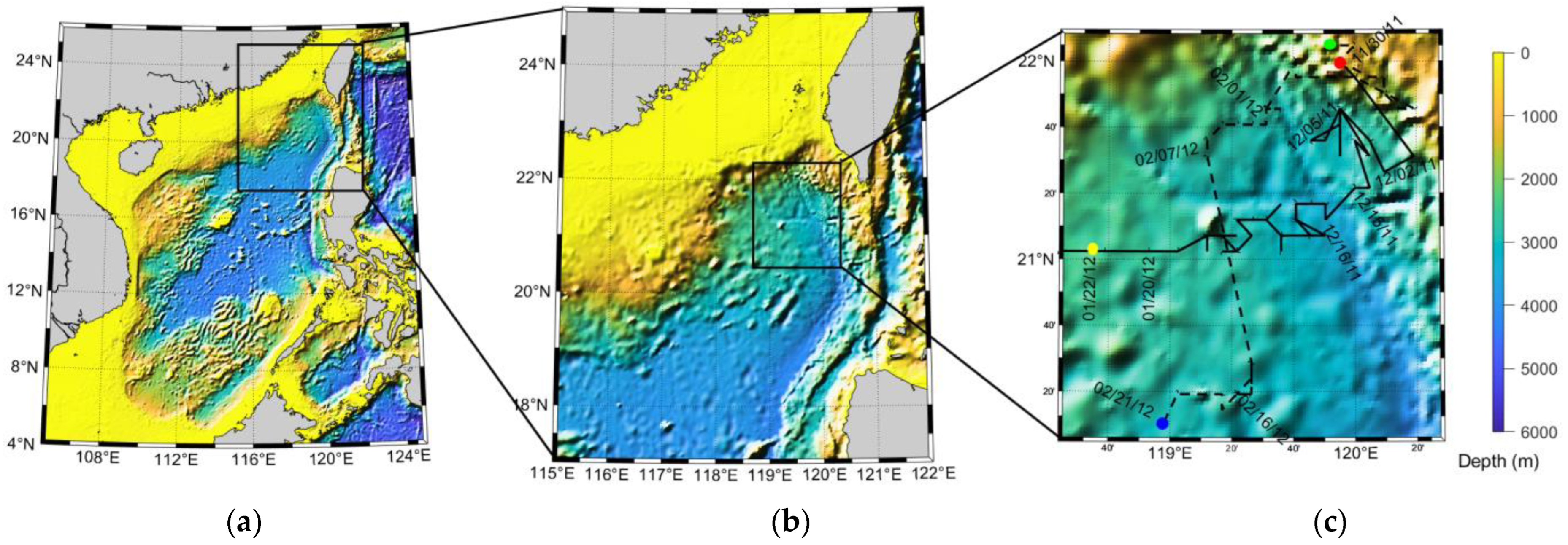
The area considered is located in the north of the South China Sea, as shown in the topographic map in Figure 1. The horizontal resolution of the data is 1/12°, i.e., 7.6 km. In longitude and latitude, 27 points are chosen, covering an area of 200 km $\times$ 200 km. The HYCOM data have 37 layers in vertical depth, ranging from 0 m to 2500 m, with an unequal grid. Here, depth grids are interpolated to have a resolution of 10 m, thus resulting in 251 points. Consequently, the 3D SSF has a grid size of $27\times 27\times 251$. The data are from 6 November 2011 to 20 March 2012, across 136 days.

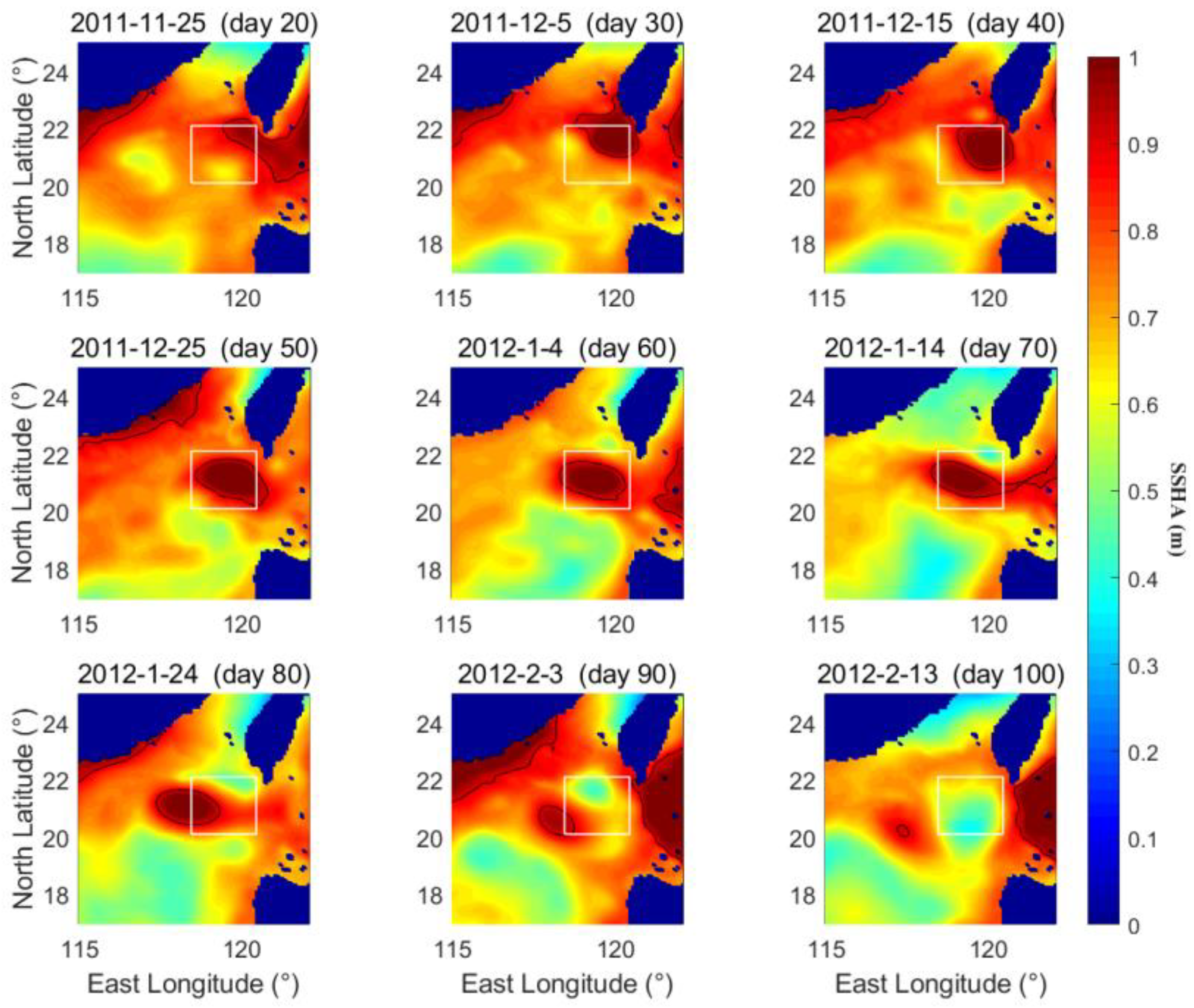
An aerial view of the whole of the South China Sea is shown in Figure 1a. The northwest of the South China Sea is enlarged in Figure 1b. The area in Figure 1c is the SSF reconstruction area. The sea surface height anomaly (SSHA) data during this period were measured by satellites, as shown in Figure 2, which has the same area in Figure 1b. During this period, a warm eddy (anticyclone) and a cold eddy (cyclone) are moving across the region, as seen in Figure 2. The 0.9 m contour line reflects the mesoscale warm eddy. The warm eddy center is identified by the maximum of the SSHA contour. It can be seen from Figure 2 that the mesoscale warm eddy moves southward into the area in the 25th day, 30 November 2011, center dotted by red circle in Figure 1c. Then it moved westward from the 40th day, 15 December 2011, along the latitude of about 21.2°N. It almost locates at the center of the area in the 60th day, 4 January 2012. It moves out of the area in the 78th day, 22 January 2012, center dotted by yellow circle in Figure 1c. The locations of the eddy center are shown in Figure 1c and the trajectory of the warm eddy center is plotted by the black line. The cold eddy enters into the area in the 68th day, 12 January 2012, center dotted by green circle in Figure 1c. The cold eddy moves out of the area in the 108th day, 21 February 2012, center dotted by blue circle in Figure 1c.

To clearly show the 3D SSF variations by the warm mesoscale eddy, the 40th, 60th, and 80th day 3D SSFs are demonstrated in Figure 3, with the 3D structure of the warm mesoscale eddy being highlighted by black dashed lines. From the highlighted areas, it can be observed that the inducing positive sound speed anomalies lie in the depth of 100 m to 700 m. The cold eddy is also shown in the corner of Figure 3c, side by side with the warm eddy.

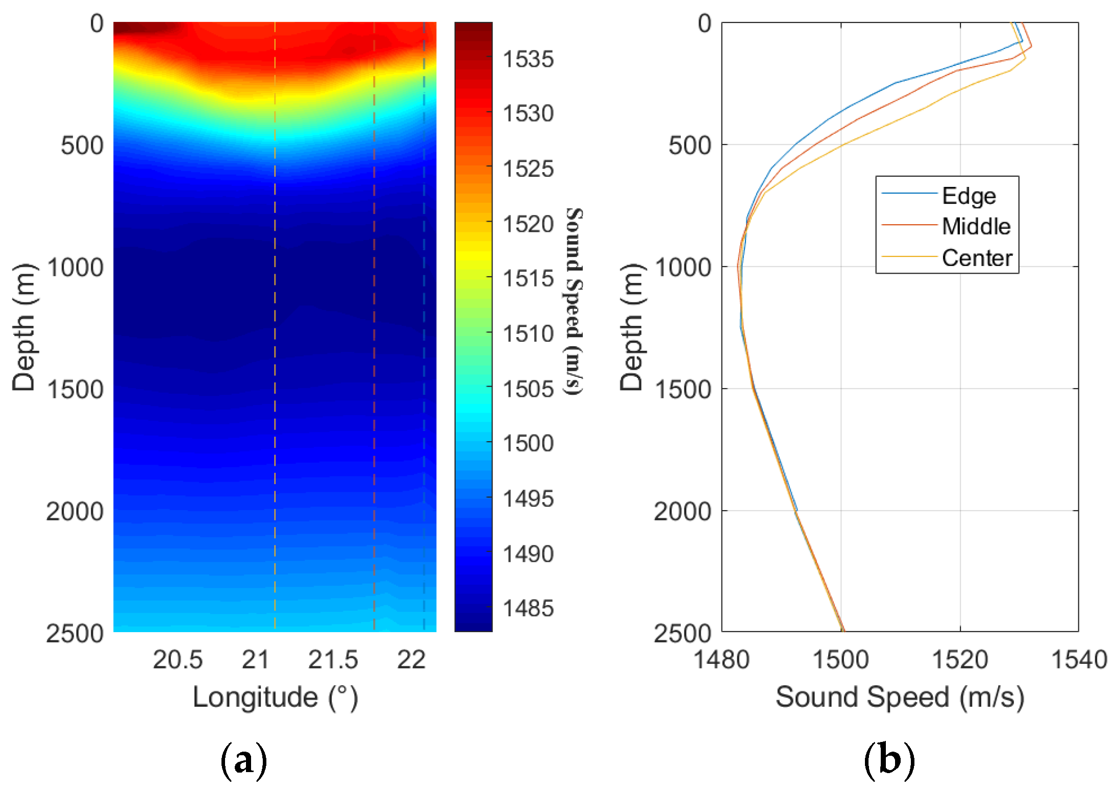
We take a closer look at one section in Figure 3b. Taking one section from the 3D SSF on the 60th day at 119.44°E, the 2D SSF can be seen as a cross section of the mesoscale eddy in Figure 4a. The isosonic line is downward, indicating a warm eddy in the area since the warm eddy leads to positive sound speed anomalies compared with the nominal. It can be seen that there are significant differences among the SSPs, mainly below the mixing layer and above 700 m. The eddy center has the highest sound speed, and the sound speed gradually decreases towards the edge of the eddy, as seen in Figure 4b.

The methods for reduced-order representation include vertical representation and horizontal representation. EOF is most widely used as a vertical basis function.

2.2. Reduced-Order Representation Methods Review

Here, the 3D SSF ${\{c(x,y,z)\}}_{x=1,y=1,z=1}^{M,N,I}$ refers to the sound speed distribution in a 3D space at a single time. $x,y,z$ represent longitude, latitude, and depth, respectively. $M, N, I$ are the number of grids in longitude, latitude, and depth, respectively.

The 3D SSF contains the mean part (range-independent) and perturbation part (range-dependent). The mean SSP is the zeroth order basis function while perturbation can be expressed as a sum of modal basis functions. Horizontal stratification characteristics in the deep ocean are well known, due to the significant differences between the horizontal and vertical scales of the ocean. Therefore, the 3D representation in the vertical dimension (depth) and horizontal dimensions (longitude and latitude) are separately treated, taking the following form:

$$c(x,y,z)=c(z)+{\displaystyle \sum _{j=1}^{N_{xy}}{\displaystyle \sum _{i=1}^{N_z}{w}_{ij}{\left[F(x,y)\right]}_j{\left[E(z)\right]}_i}},$$

(2)

where $c(z)$ is the mean SSP, ${\left[F(x,y)\right]}_j$ is the j-th horizontal basis function and ${\left[E(z)\right]}_i$ is the i-th vertical basis function. $N_{xy}$ and $N_z$ denote the number of basis functions for horizontal and vertical axes, respectively.

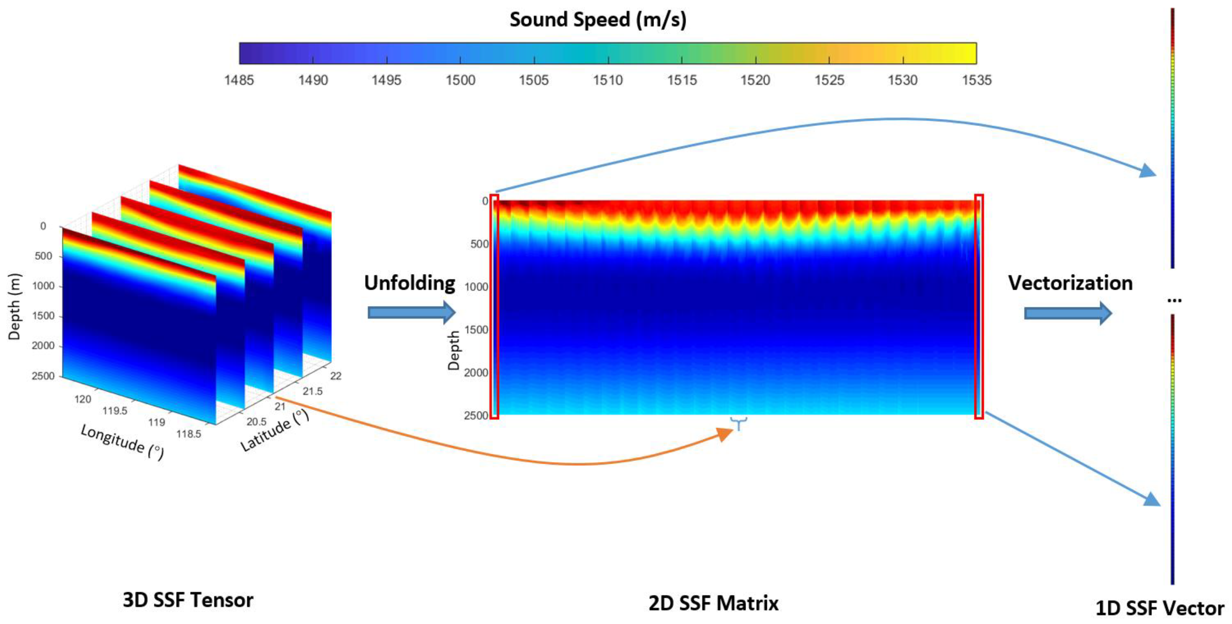
Based on the above numerical analysis, we further express the de-mean 3D SSF in the form of tensor, matrix, and vector. The tensor form of 3D SSF is expressed as $\chi \in {ℝ}^{M\times N\times I}$. Stacking the longitude–depth slice (mode–latitude unfolding), the tensor will be unfolded into a matrix as $X\in {ℝ}^{I\times MN}$. Expanding the matrix by depth (column vectorization), the matrix will be vectored as $x\in {ℝ}^{IMN\times 1}$. That is, a 3D SSF can be expressed as $\chi$, $X$, $x$ in the form of tensor, matrix, and vector, respectively. The relationship between them is

$$\mathrm{unfolding}(\chi )=X,$$

(3)

$$\mathrm{vec}(X)=x,$$

(4)

where unfolding means mode–latitude unfolding and vec means column vectorization. A sketch map of the transforms is shown in Figure 5.

2.2.1. SSP Representation and EOF

The empirical orthogonal function (EOF) is the most widely used basis function in the vertical dimension. EOFs are empirical modes calculated by historical sound speed profiles. It is a pure data-driven reduced-order method. The calculation of EOFs will be described after the matrix definition of 3D SSF.

The calculation of EOFs is drawn from the SVD decomposition of a set of SSPs. The commonly used method is to calculate the covariance matrix for principal component analysis (PCA), that is, eigenvalue decomposition.

At first, the mean SSP is calculated. The mean of 3D SSF $Y\in {ℝ}^{I\times MN}$ is $m=(1/MN){\displaystyle \sum _{j=1}^{MN}{y}_j}\in {ℝ}^{I\times 1}$. A mean matrix is constructed by $M=[m,\dots ,m]\in {ℝ}^{I\times MN}$. Subtract $M$ from $Y$ and resulting the de-mean 3D SSF matrix

$$X=\left[x_1,\dots ,x_{MN}\right]=Y-M\in {ℝ}^{I\times MN}.$$

(5)

Eigenvalue decomposition of the covariance matrix of $X$ is

$$X{X}^{\mathrm{T}}=E\Lambda E^{\mathrm{T}},$$

(6)

where $E=\left[e_1,\dots ,e_I\right]\in {ℝ}^{I\times I}$ and $\Lambda =\mathrm{diag}\left(\left[{\lambda }_1,\dots ,{\lambda }_I\right]\right)$ with decreasing eigenvalues ${\lambda }_1\ge \cdots \ge {\lambda }_I$. In practice, the first K of I eigenvectors are generally taken for reduced-order representation with $K\ll I$. The truncated SVD decomposition is expressed as $X{X}^{\mathrm{T}}\approx E_K{\Lambda }_K{E}_K^T$, where ${\Lambda }_K=\mathrm{diag}\left(\left[{\lambda }_1,\dots ,{\lambda }_K\right]\right)$ and

$$E_K=\left[e_1,\dots ,e_K\right]\in {ℝ}^{I\times K}.$$

(7)

The selection rule of $K$ is generally as ${\displaystyle \sum _{i=1}^K{\lambda }_i}/{\displaystyle \sum _{i=1}^I{\lambda }_i}$ greater than a certain threshold, which can be taken as 90% or 99%. The empirical value of $K$ in the literature is 2 to 6 [28,29,30]. The 3D SSF matrix is expressed as

$$X\approx E_{K}W,$$

(8)

where $W\in {ℝ}^{K\times MN}$ is the matrix of representation coefficients. Since the EOF matrix $E_K$ satisfies orthogonality (e.g., $E_K^{\mathrm{T}}{E}_K=I_K$), the coefficients matrix can be obtained by

$$\widehat{W}=E_K^{\mathrm{T}}X.$$

(9)

2.2.2. 3-D SSF Representation

Furthermore, the orthogonality assumptions are applied for horizontal dimensions in x and y, and we can separate basis functions in x and y, as

$$c(x,y,z)=c(z)+{\displaystyle \sum _{k=1}^{N_x}{\displaystyle \sum _{j=1}^{N_y}{\displaystyle \sum _{i=1}^{N_z}{w}_{ijk}{\left[F_1(x)\right]}_k{\left[F_2(y)\right]}_j{\left[E(z)\right]}_i}}},$$

(10)

where ${\left[F_1(x)\right]}_{k=1}^{N_x}$ is the basis function in the x-axis (longitude) and ${\left[F_2(y)\right]}_{j=1}^{N_y}$ in the y-axis (latitude), with a total of $N_x$ and $N_y$, respectively.

A.

Spectral-analysis Method

Two-dimensional Fourier decomposition is often used to represent the horizontal dimensions of 3D SSF. As horizontal basis functions, Fourier basis are a reduced-order method of spectral analysis, which use exponential basis as structural modes. The 3D reduced-order representation using horizontal two-dimensional Fourier basis and vertical EOF basis can be expressed as

$$c(x,y,z)={\displaystyle \sum _{f_1=1}^{N_{F_1}}{\displaystyle \sum _{f_2=1}^{N_{F_2}}{\displaystyle \sum _{k=1}^{K_F}{w}_{f_1,f_2,k}}}}\underset{1\mathrm{D} \mathrm{EOF}}{\underbrace{{\left[E_{K_F}\right]}_{z,k}}}\times \exp \left(2\pi j\left[\frac{x\left(f_1-1\right)}{L_x}\right]\right)\exp \left(2\pi j\left[\frac{y\left(f_2-1\right)}{L_y}\right]\right),$$

(11)

where ${\left[E_{K_F}\right]}_{z,k}$ is the z-th depth and the k-th order EOF. $K_F$ is the number of EOFs for z-axis. $N_{F_1}$ and $N_{F_2}$ denote the number of Fourier basis functions for the x-axis and y-axis.

For a 3D SSF, ${\left\{c^{*}(x,y,z)\right\}}_{x=1,y=1,z=1}^{M,N,I}$, the representation coefficients ${\left\{w_{f_1,f_2,k}^{*}\right\}}_{f_1=1,f_2=1,k=1}^{N_{F_1},N_{F_2},K_F}$ can be expressed in matrix form as

$${\widehat{X}}^{*,\mathrm{u}}=E_{K_F}{W}^{*}{F}^{\mathrm{T}},$$

(12)

$$W^{*}=E_{K_F}^{\mathrm{T}}{X}^{*,\mathrm{u}}{\left(F^{\mathrm{T}}\right)}^{†},$$

(13)

where $X^{*,\mathrm{u}}\in {ℝ}^{I\times MN}$ is 3D SSF in matrix form and $W^{*}\in {ℝ}^{K_F\times N_{F_1}{N}_{F_2}}$ is the matrix of representation coefficients. $F_1$ and $F_2$ are Fourier basis matrices and $F=F_2\otimes F_1\in {ℂ}^{MN\times N_{F_1}{N}_{F_2}}$. The expression of $F_1$ and $F_2$ are listed in Appendix A. Henceforth, the method proposed in this subsection is named Fourier + EOF.

B.

Data-Driven Method

A fully data-driven method for 3D SSF reduced-order representation is described here, which learns all of the basis functions in three directions from data.

Assuming the basis functions of the three dimensions are orthogonal to each other, the basis functions can be obtained by tensor decomposition CPD. Here, we use the higher-order orthogonal iteration (HOOI) algorithm [9]. The specific calculation algorithm can be found in the reference and will not be listed here. The theory insight of orthogonal tensor decomposition shows that it is a universal 3D representation method. The depth basis functions learned from HOOI are the same as EOFs.

The decomposition of HOOI can be expressed as

$$\mathcal{X}=\mathcal{S}{\times }_1{B}^{(1)}{\times }_2{B}^{(2)}{\times }_3{B}^{(3)},$$

(14)

where $\mathcal{S}\in {ℝ}^{L_1\times L_2\times L_3}$ is core-tensor with a size of $L_1\times L_2\times L_3$, $B^{(1)}\in {ℝ}^{M\times L_1}$, $B^{(2)}\in {ℝ}^{N\times L_2}$, $B^{(3)}\in {ℝ}^{I\times L_3}$ are basis functions in longitude, latitude, and depth, respectively, and ${\times }_p$ means mode-p product. Henceforth, the method proposed in this subsection is named HOOI.

For a reconstructed 3D SSF $\widehat{\chi }, \widehat{X}, \widehat{x}$ in the form of tensor, matrix and vector respectively, the reconstruction error is expressed by RMSE (root mean square error) of each grid point, that is

$$\mathrm{RMSE}=\frac{1}{\sqrt{MNI}}{\Vert \widehat{\chi }-\chi \Vert }_F=\frac{1}{\sqrt{MNI}}{\Vert \widehat{X}-X\Vert }_F=\frac{1}{\sqrt{MNI}}{\Vert \widehat{x}-x\Vert }_2.$$

(15)

2.3. RBF and Physics-Guided Representation Method

The radial distance refers to the distance related to the position and unrelated to the direction. The radial distance between the data point $\overrightarrow{p}$ and the measurement point ${\overrightarrow{p}}_0$ is $r=\phi (\overrightarrow{p}-{\overrightarrow{p}}_0)$. In general, Euclidean distance is used as the radial distance $r=\Vert \overrightarrow{p}-{\overrightarrow{p}}_0\Vert$ where $\Vert \Vert$ is l-2 norm of the vector.

RBF is a function of radial distance. Here, we use Gaussian RBF which takes the exponential weighted sum of the reciprocal of radial distance as the interpolation function. The weighting function is

$$\phi (r)=\exp (-\frac{r^2}{2R_0{}^2}),$$

(16)

where $R_0$ is the width of RBF, representing the range and distribution in the input space.

In physical oceanography, the universal structure of a mesoscale eddy is expressed as $p_{\mathrm{n}}\left(r_{\mathrm{n}},z\right)=R\left(r_{\mathrm{n}}\right)\cdot H(z)$ where $R\left(r_n\right)=\left(1-r_n^2/2\right)\cdot \exp \left(-r_n^2/2\right)$ and $r_{\mathrm{n}}=r/R_m$. $p_{\mathrm{n}}$ is pressure anomaly, $r_{\mathrm{n}}$ is the normalized range, $r$ is the range, $R_m$ is the radius of mesoscale eddy and $z$ is depth. Thus, the horizontal structure of the mesoscale eddy is expressed as

$$R\left(r\right)=\exp \left(-r^2/2R_m{}^2\right).$$

(17)

In the subsequent discussion, we will use the radius (a concept in the mesoscale eddy model) as the width (a concept in RBF) to emphasize the physical meaning of width. However, it should be noted that in the RBF interpolation, the optimal $R_0$ is not equal to the radius $R_m$ of the mesoscale eddy. The 3D SSF includes various ocean phenomena including mesoscale eddy affecting SSF. It can be evaluated that the radius is related to the order of RBF.

The Gaussian RBF is expressed as

$$\mathsf{\Phi }(r)={\displaystyle \sum _{p=1}^P{w}_p\phi (r_p)}={\displaystyle \sum _{p=1}^P{w}_p\phi \left[\exp (-\frac{r_p{}^2}{2R_0{}^2})\right]},$$

(18)

and in matrix form as

$$\mathsf{\Phi }(P)={\displaystyle \sum _{p=1}^P{w}_p\phi (\Vert P-P^p\Vert )}={\displaystyle \sum _{p=1}^P{w}_p\exp (-\frac{1}{2R_0{}^2}{\Vert P-P^p\Vert }^2)},$$

(19)

where $P$ indicate the points to be interpolated and $P^p$ are the RBF centers. Here, $P\in {ℝ}^{MN\times 2}=\left[p_{\mathrm{x}},p_{\mathrm{y}}\right]$ are all discrete longitude and latitude grids in the reconstructed region, with longitude vector $p_{\mathrm{x}}\in {ℝ}^{MN\times 1}={[p_{x_1},p_{x_2},\dots ,p_{x_{MN}}]}^{\mathrm{T}}$ and latitude vector $p_{\mathrm{y}}\in {ℝ}^{MN\times 1}={[p_{y_1},p_{y_2},\dots ,p_{y_{MN}}]}^{\mathrm{T}}$. $P^p$ are selected center points from $P$, with a total number of $P$ while $P<MN$. $w_p$ is the weighting coefficient of p-th RBF. The matrix form of $\Phi \in {ℝ}^{MN\times P}$ is,

$$\Phi =\left[\begin{array}{cccc}{\phi }_{11}& {\phi }_{12}& \cdots & {\phi }_{1P}\\ {\phi }_{21}& {\phi }_{22}& \cdots & {\phi }_{2P}\\ ⋮& ⋮& & ⋮\\ {\phi }_{[MN]1}& {\phi }_{[MN]2}& \cdots & {\phi }_{[MN]P}\end{array}\right],$$

(20)

where

$${\phi }_{ip}=\phi (\Vert P^i-P^p\Vert )=\exp (-\frac{1}{2R_0{}^2}{\Vert P^i-P^p\Vert }^2),$$

(21)

where i indicates the i-th row in $P\in {ℝ}^{MN\times 2}$ and p indicates p-th RBF center $P^p$.

The inverse of $\Phi$ is solved by pseudo inverse, because $\Phi$ is not orthogonal, is derived by

$${\Phi }^{†}={({\Phi }^T\Phi )}^{-1}{\Phi }^{\mathrm{T}}.$$

(22)

In the matrix form of 3D SSF representation, the coefficients and reconstructed 3D SSF is shown as

$$W^{*}=E_{K_F}^{\mathrm{T}}{X}^{*,\mathrm{u}}{\left({\Phi }^{\mathrm{T}}\right)}^{†},$$

(23)

$${\widehat{X}}^{*,\mathrm{u}}=E_{K_F}{W}^{*}{\Phi }^{\mathrm{T}}.$$

(24)

In the vector form of 3D SSF representation, and define $w^{*}\equiv \mathrm{vec}(W^{*})$, $x^{*,\mathrm{u}}\equiv \mathrm{vec}(X^{*,\mathrm{u}})$, the Eq above can be expressed as [31]

$$x^{*,\mathrm{u}}=(\Phi \otimes E_{K_F})w^{*}.$$

(25)

The order reduction of RBF representation is due to $P<MN$. There are two rules for the selection of $P^p$, including random selection and regular selection. Random selection refers to a random selection of points among all grid points while regular selection refers to the selection of points in the region that are equally spaced in each direction. In addition, the center of RBF can be learned by clustering methods, which is an adaptive self-organized algorithm. If the central positions of the mesoscale eddies are known, this point can be selected. The central position of the mesoscale eddies generally can be obtained from the satellite altimeter data, before taking charge of the underwater 3D SSF data.

The width $R_0$ of RBFs is selected as a scalar here, that is, each order of RBF has the same width, as well as isotropic RBFs. $R_0$ is learned from historical data, which is the correlation radius of the SSF. The radius is near the radius of the mesoscale eddy, ranging from 50 km to 200 km. Empirically, the radius can be selected as 100 km. Henceforth, the method proposed in this subsection is named RBF + EOF.

3. Results and Discussion

In this section, we interpret the theory of the RBF + EOF method in a physical and data sense, evaluate the performance and discuss the parameters of the proposed method, compared with benchmarking methods for 3D SSF reduced-order representation.

3.1. Theoretical Interpretation and First-Order RBF + EOF

Previously, there has been some literature accounting for the universal 3D structure of mesoscale eddies such as [12,14], which both use the Gaussian function in horizontal dimensions, indicating the physical guide of representing mesoscale eddies. Particularly, the Gaussian eddy model [14] links the 3D SSF structure and the mesoscale eddy for the first time, exploring the universal 3D SSF anomaly distribution feature. The Gaussian eddy model represents one mesoscale eddy by one-order Gaussian approximation.

RBF + EOF is the representation method proposed by us, which can represent and reconstruct the 3D SSF. It is suitable for 3D SSF representation containing various ocean phenomena including mesoscale eddies. RBF + EOF is a physics-guided eddy representation model. In theory, the first-order RBF + EOF is physically inextricably linked to the Gaussian eddy model. The formulation of the Gaussian eddy model and the first-order RBF + EOF are listed below for comparison.

The Gaussian eddy model [14] can be expressed as

$$\Delta c(x,y,z)=\Delta c_{\max }\exp (-\frac{{(\sqrt{x^2+y^2}-r_c)}^2}{D_r{}^2})\exp (-\frac{{(z-z_c)}^2}{D_z{}^2}),$$

(26)

The first-order RBF + EOF is characterized by setting $K_F=1$ in Equation (24) and $P=1$ in Equation (20) as

$$\Delta c(x,y,z)=w_{11}\exp (-\frac{{(\sqrt{x^2+y^2}-r_c)}^2}{R_0{}^2}){\left[E(z)\right]}_1,$$

(27)

We can find both of them have a similar form, especially since the exponential term is almost the same as $D_r=R_0$. The horizontal structures are both in Gaussian form, which indicates that the Gaussian RBF is a physics-guided universal structure in 3D SSF representation for mesoscale eddies. The relation between the first-order RBF + EOF method and the Gaussian eddy model has been viewed in a physical and mathematical sense, and the difference in depth dimension term is further explained by numerical simulation using HYCOM data.

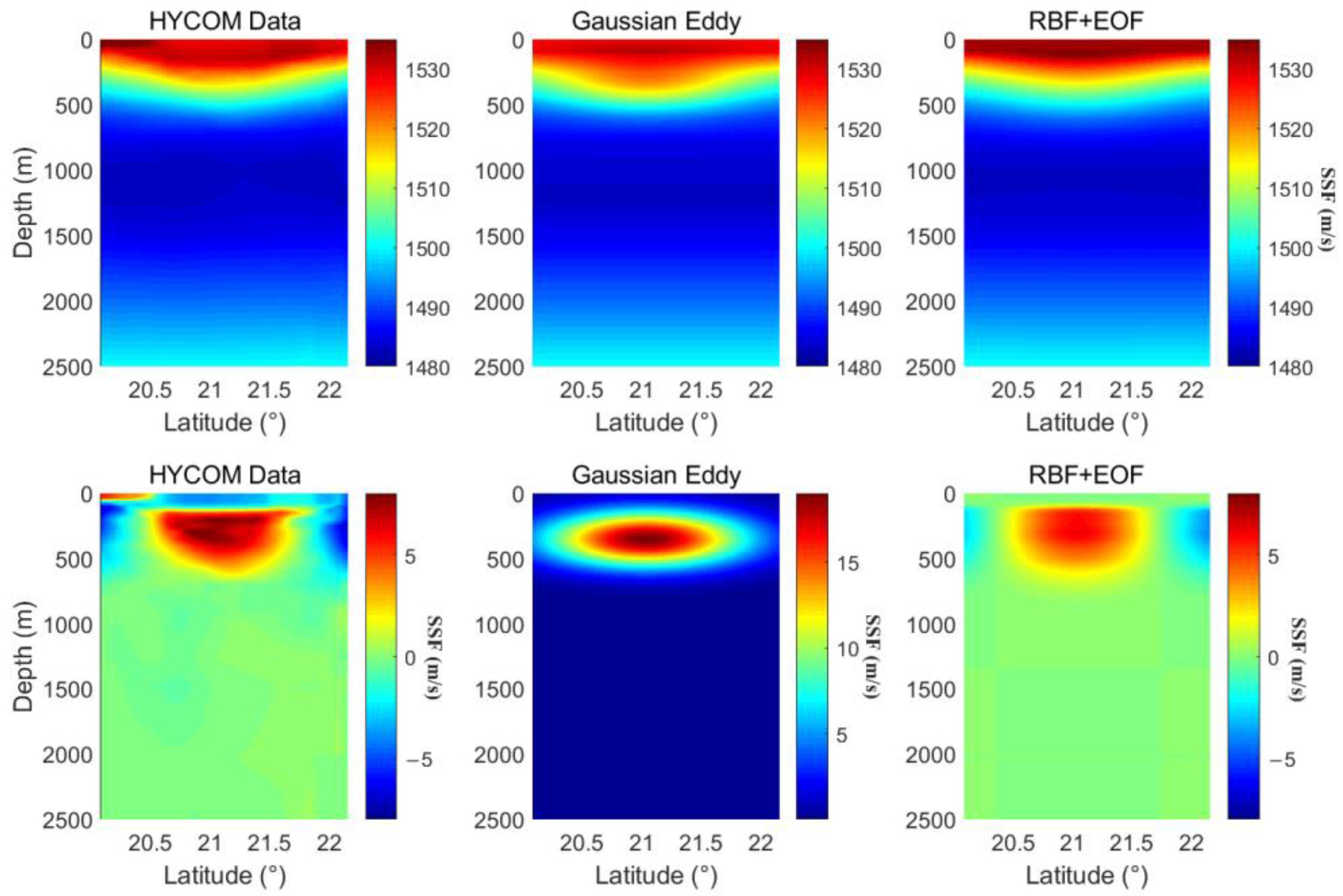
3D SSF data on the 60th day are used to reconstruct by the Gaussian eddy model and the first-order RBF + EOF, respectively. The parameter is set to $P=N_{E_K}=1$, $D_r=R_0=80 \mathrm{km}$, $z_c=350 \mathrm{m}$, the longitude and latitude of $r_c$ is 21.04°N, 119.36°E. As shown in Figure 6, for the horizontal section of the 3D SSF, the Gaussian eddy model and RBF have the same structure, which are both Gaussian approximations of the original data. As shown in Figure 7, the vertical profile of EOF and Gaussian eddy are similar, which is the fitting and smoothing of the original HYCOM data. The Gaussian eddy has a symmetrical structure of the center depth $z_c$, which is slightly deeper than the actual value. The true eddy has a nonsymmetrical structure of the center depth, which is learned by EOF, showing the ability to learn features from data.

As shown in Figure 8, the vertical slices of 3D SSF reconstructed by the Gaussian eddy model and the first-order RBF + EOF are compared. The RMSE of Gaussian eddy and RBF + EOF are 1.46 m/s and 1.32 m/s, respectively. Their performances are basically similar. Considering the slight difference between them, RMSE of RBF + EOF is slightly lower because the eddy in HYCOM data has the shape of a bowl rather than a ball, and the error of EOF is relatively smaller than the Gaussian eddy model. According to simulation results, the performance of the first-order RBF + EOF is significantly superior from the 40th to 60th day. During this period of time, the mesoscale eddy is completely located in the reconstruction area (as shown in Figure 2), indicating that the first-order RBF + EOF has a pretty representation performance to characterize the 3D SSF dominated by one mesoscale eddy.

According to the above analysis, we conclude that the first-order RBF + EOF can be regarded as an approximation of the Gaussian eddy model. The first-order RBF is completely consistent with the horizontal Gaussian eddy model. The first-order EOF represents the vertical characteristics of mesoscale eddy learned from the data while the Gaussian eddy model is structured as a Gaussian shape with two parameters.

3.2. Multi-Order RBF + EOF Representation Method and Parameters Selection

In this subsection, we introduce the multi-order RBF + EOF representation method and show its representation results. The parameters selection of different parameters for RBF + EOF is discussed, including the position of RBF center points, the order of RBF, and the width of RBF. This section uses the data from the first day for testing.

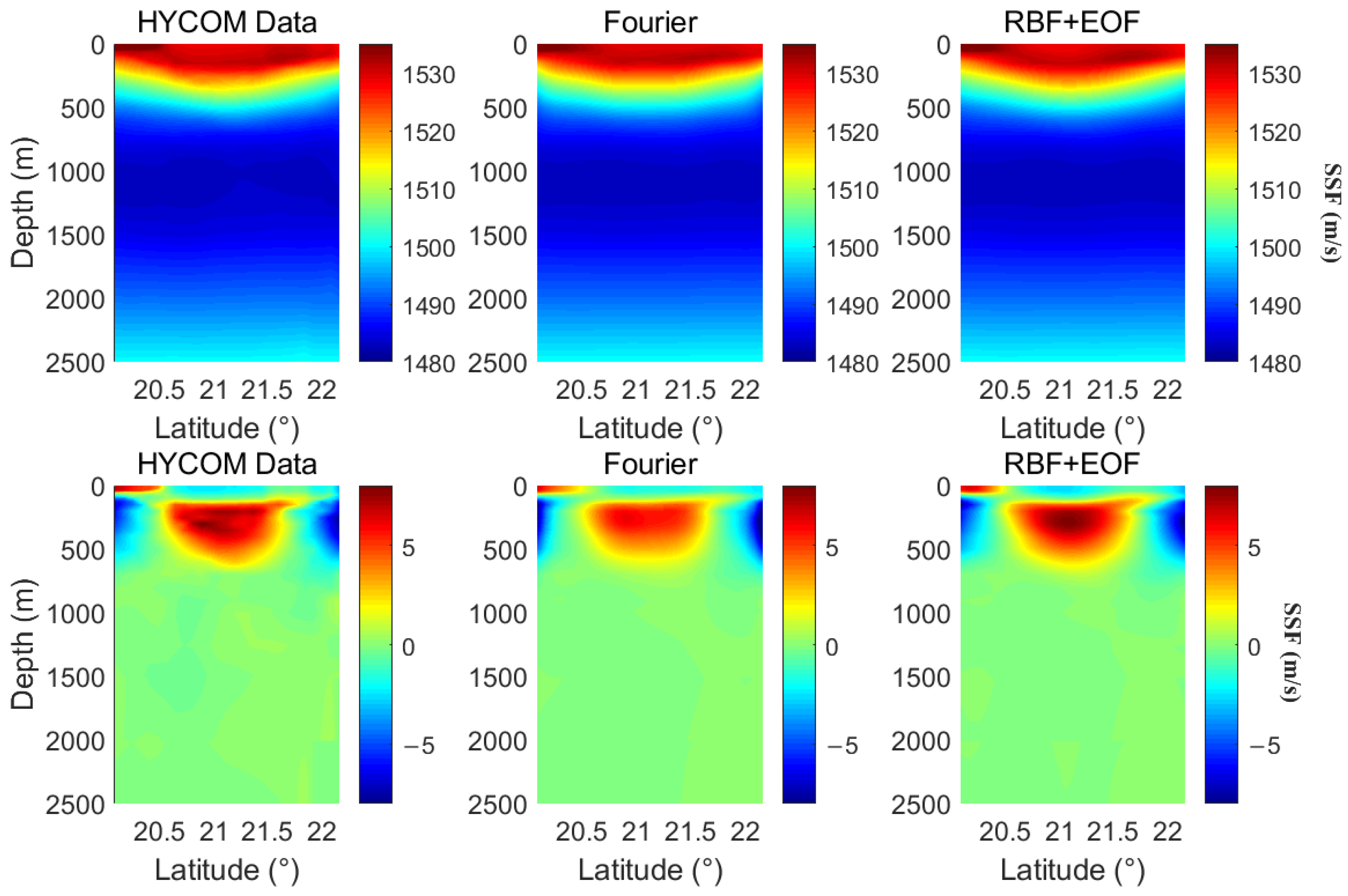
We use the 3D SSF data on the 60th day to represent 3D SSF, similar to Section 3.1, with the multi-order RBF + EOF method and the Fourier + EOF method. The parameters are set to $N_{E_K}=6$, $N_{F_1}\times N_{F_2}=P=36$, $R_0=80 \mathrm{km}$. The center of RBFs is randomly selected. As shown in Figure 9, the 36-order RBFs represent the mesoscale more accurately in horizontal dimensions, compared with the first-order RBF in Figure 6. The vertical slice of a mesoscale eddy representation using multi-order RBF + EOF in Figure 10 is more delicate compared with the first-order RBF + EOF in Figure 8. The Fourier method in Figure 9 and Figure 10 has less recoverable detail compared with multi-order RBF + EOF, especially near the center of the eddy.

Considering the amount of calculation, the pseudo inversion of matrix $\Phi$ in Equation (22) is dominating. The amount of calculation for the multi-order $P$ RBFs inversion is $P$ times of first-order RBF, which takes much time. In practice, the pseudo inversion for a matrix with size of 27 $\times$ 27 and $P=100$ times only takes 0.02 s. This procedure can be calculated and saved in advance to save time. Once the basis functions are calculated, in the following representation, pseudo inversion will not be repeated.

In the above simulation, the representation performance of the multi-order RBF + EOF method for the 3D SSF dominated by one mesoscale eddy is qualitatively evaluated. The quantitative performance and robustness of more complex 3D SSF will be evaluated in the next subsection, such as the 90th day including two mesoscale eddies. Afterward, parameters selection will be carried out.

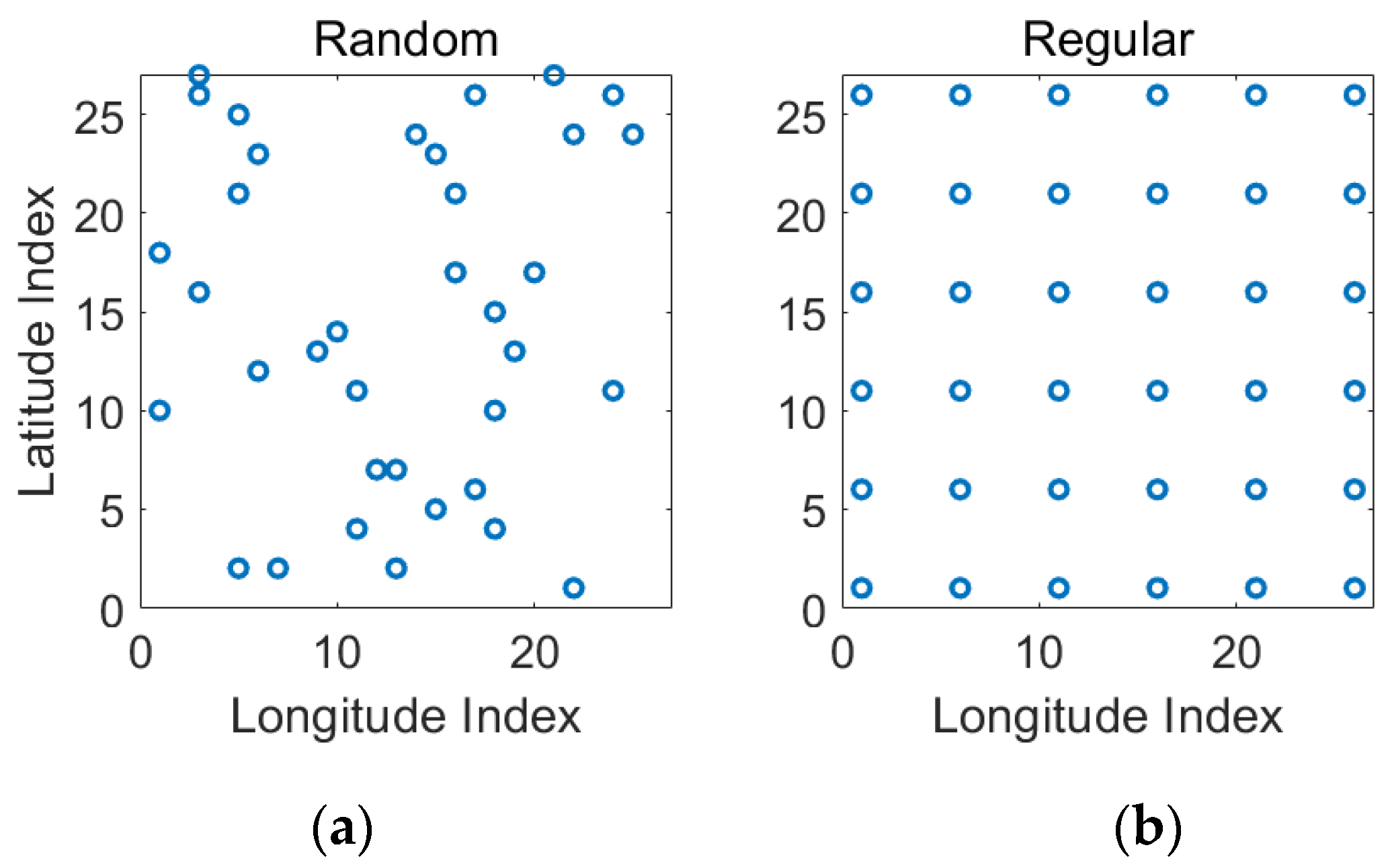
For the position’s selection of $P$ RBF center points, there are two rules, random selection, and regular selection. Regular selection refers to equally spaced points in the area being selected which makes the distribution of RBF centers uniform space. Take 36 orders of RBF as an example. Figure 11 shows the 36 points (blue circle) by random selection and regular selection in the two-dimensional horizontal region, where the horizontal and vertical axis represent the longitude and latitude grid points of the area to be reconstructed with grid size 1/12°.

The position of RBF centers will affect the performance of 3D SSF representation. We compare RBF center positions selected by different rules, including random selection and regular selection. Random selection will select P points in the area randomly and 100 Monte Carlo experiments are carried out. It can be seen from Figure 12 that the average performance of random selection is almost consistent with that of regular selection. The specific performance of random selection is related to the SSF data. As shown in the error bar in Figure 12, the performance of random selection may be better or worse than regular selection, while the latter always achieves a robust performance. In the case of low-order RBF order, the performance gap of random selection is large. Thereafter, the optimal center point needs to be obtained by other algorithms. As the order of RBF increases, the error bar gradually decreases to zeros. In the case of high-order RBF (for example, in the region of 200 km, the RBF is greater than 36 orders), the selection of the center point has little impact on the reconstruction performance, which indicates the selection rules of RBF centers will not be a key issue. Therefore, 36-order RBFs will be selected as a reference.

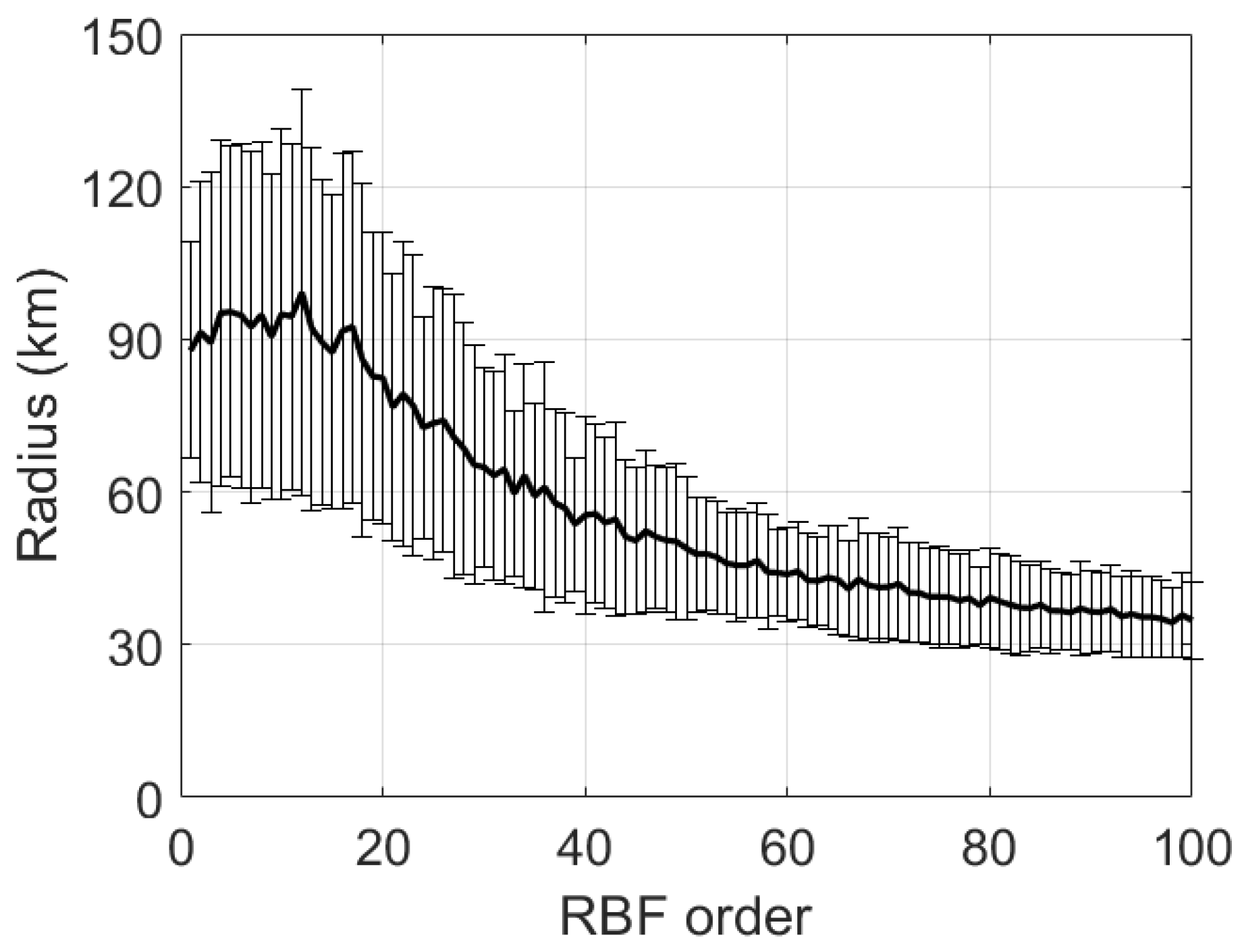
For different orders of RBF, the optimal radius $R_0$ is different. We test the 3D SSF data on the first day using 6 EOFs. As shown in Figure 13, with the increase of RBF order, the mean optimal radius (thick black line) gradually decreases from 90 km to 40 km, and the variance (thin line, error bar in figure) also decreases. This result is in conformity with the theory because with the increase of the number of RBF centers, the region represented by each order of RBF gradually converges from the global area to the local point. If the RBF center takes all grid points in the reconstruction area, the radius should be infinite so that the scale factor is zeros, that is, each order of RBF is equal to the value of the local point. This theory is called the Nadaraya–Watson regression estimator (NWRE) [32]. Within a value range, the radius is not very sensitive to RMSE. Whether 60 km or 80 km, the RMSE is very close, which indicates the radius is relatively robust. Therefore, 80 km will be selected as a reference radius for all simulations, which balances the performance of different RBF orders.

3.3. Mesoscale 3D SSF Experiment

In this section, we evaluate the performances of the RBF + EOF method, the Fourier + EOF method [8], and the tensor decomposition-based method (HOOI) [9], all in a long time period (136 days) data. We also compare the number of coefficients and performance.

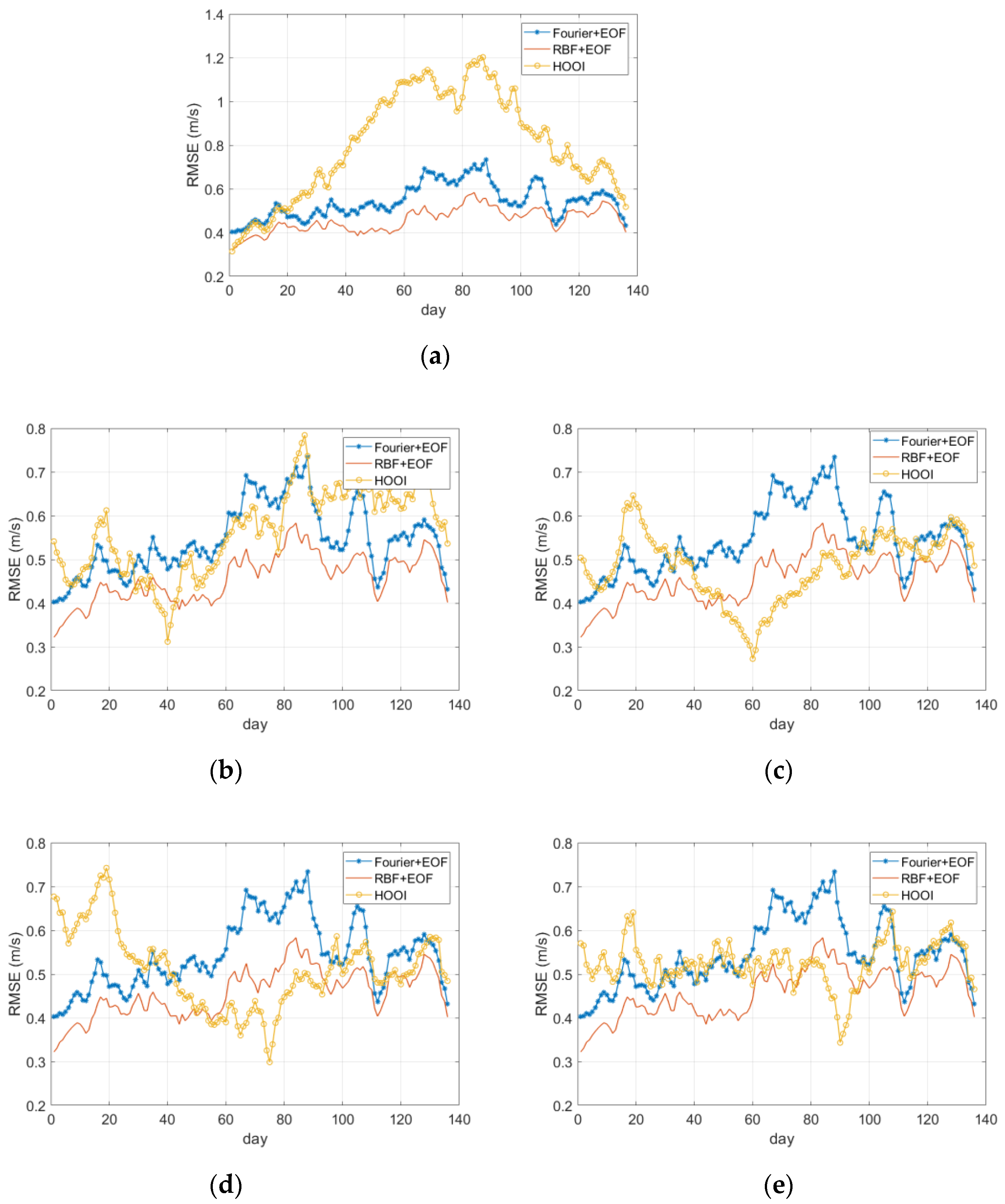
We tested 136 days of the 3D SSF data using all mentioned methods and calculated the RMSE. The parameter setting is shown in

Table 1. Parameters settings.

Method	RBF + EOF	Fourier + EOF	HOOI
Parameters	$P=36, N_{E_K}=6$	$N_{F_1}=N_{F_2}=6, N_{E_K}=6$	$L_1=L_2=L_3=6$
The Number of Coefficients	216	216	216

. As shown in Figure 14, the performance of RBF + EOF is always better than Fourier + EOF, especially in the range from the 40th to the 90th day. Although the performance of all methods decreased from the 60th to the 90th day, RBF + EOF has more advantages than Fourier + EOF. The performance of HOOI is related to the selection of training data. As shown in Figure 14a–e the training data are the first, 40th, 60th, 75th, and 90th day, respectively, which has the smallest RMSE on the training day. When the training data of HOOI is the first day (training data without eddy) as shown in Figure 14a, RMSE of HOOI is greater than that of other methods in all subsequent days and increases linearly from the first day to the 60th day. That is due to the first day data not containing mesoscale eddies, and HOOI learning no effective basis functions related to mesoscale eddies. When the training data is set as the 40th day (training data with a warm eddy), shown in Figure 14b, the RMSE in the 40th day and adjacent days are smaller than that of other methods, but the performance will be worse than that of RBF + EOF for most of the period, especially in the beginning (from the first day to the 20th day) and end period with cold mesoscale eddy (from the 90th day to the 136th day). When the training data is set as the 90th day (training data with a cold eddy) shown in Figure 14e, the RMSE in the 90th day and adjacent days are smaller than that of other methods, similar to the trend in Figure 14b. The results of other days shown in Figure 14c,d have a similar situation, where RBF + EOF outperforms than HOOI during days without eddy, which performs robustly during the period. On most days, RBF + EOF has the lowest RMSE than HOOI regardless of the training data, while the former uses only one parameter learned from data (the radius).

The performance comparison of various methods with different parameter numbers is compared. Take the 20th day SSF data for HOOI training, and take the 60th day data for performance comparison. The radius of RBF is set as 80 km for all cases.

Firstly, we compare the role of vertical dimension parameters, shown in case1 in

Table 2. Parameters setting.

Method	RBF + EOF	Fourier + EOF	HOOI
Parameters (Case1)	$P=6^2,$ $N_{E_K}=\{2,4,6\dots 10,12\}$	$N_{F_1}=N_{F_2}=6$ $N_{E_K}=\{2,4,6\dots 10,12\}$	$L_1=L_2=6$ $L_3=\{2,4,6\dots 10,12\}$
Parameters (Case2)	$P={\{4,5\dots 11,12\}}^2$ $N_{E_K}=6$	$N_{F_1}=N_{F_2}=\{4,5\dots 11,12\}$ $N_{E_K}=6$	$L_1=L_2=\{4,5\dots 11,12\}$ $L_3=6$
The Number of Coefficients(Case1)	$\{72,144,\dots 360,432\}$	$\{72,144,\dots 360,432\}$	$\{72,144,\dots 360,432\}$
The Number of Coefficients(Case2)	$\{96,150,\dots 726,864\}$	$\{96,150,\dots 726,864\}$	$\{96,150,\dots 726,864\}$

. With fixed horizontal dimension parameters which are all 36 orders, the performance comparison of the vertical dimension parameters is taken as 2 to 12 orders, respectively. The results are shown on the left of Figure 15a. With the same number of parameters, the RMSE of RBF + EOF is smaller than the other two methods.

Then, we compare the role of horizontal dimension parameters, shown in case2 in Table 2. With fixed vertical dimension parameters which are all six orders, the performance comparison of the horizontal dimension parameters is taken as 16 to 121 (square numbers), respectively. The results are shown in Figure 15b. With same number of parameters, the RMSE of RBF + EOF is smaller than the other two methods. Especially in the case of a small number of parameters, the performance of RBF + EOF is much better than Fourier + EOF.

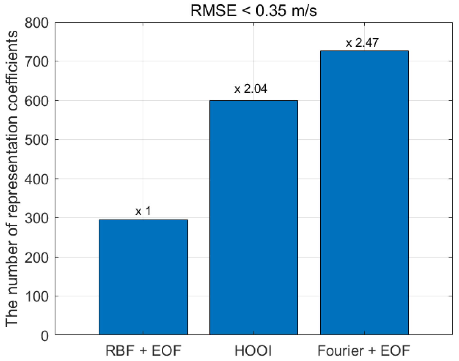
Lastly, the number of parameters required to achieve the same performance (RMSE) can be calculated. As shown in Figure 16, to achieve the goal of RMSE less than 0.35 m/s, RBF + EOF needs 296 coefficients while HOOI needs 600 and Fourier + EOF needs 726, which are 2.04 times and 2.47 times RBF + EOF, respectively. This result is based on a SSF with a mesoscale warm eddy in the center of the reconstruction area, which is state-of-the-art performance for RBF + EOF method. This shows that the proposed RBF + EOF method has good performance in the representation in the horizontal dimension, achieves acceptable RMSE with a lower number of coefficients, and can greatly reduce the degree of uncertainty in the inverse problem.

4. Conclusions

In this paper, a 3D SSF with mesoscale eddies has been considered by way of reduced-order representation with proposed effective basis functions. The physics of mesoscale eddies is connected to the RBF in a seamless physical guide and math-analytical method. The first-order RBF + EOF representation method is an approximation of the classic Gaussian eddy model. Multi-order RBF + EOF is a semi-data-driven and semi-model-driven method combining knowledge in data and in physics.

The theory interpretation between 3D SSF with mesoscale eddy and Gaussian RBF is shown and tested. The parameters of RBF are assessed in detail. The performance of the RBF + EOF method is evaluated using the reanalysis 3D SSF data in the South China Sea and compared to other benchmark methods including Fourier + EOF and tensor-based HOOI, showing robustness and accuracy in whole days. The results also indicate RBF + EOF is relatively better with a lower number of representation coefficients, which will be appropriate in acoustical oceanography.

We will use the proposed method in OAT for 3D SSF inversion and try to observe mesoscale eddies in the South China Sea [33]. Several OAT experiments have been conducted [34] and mesoscale eddies have been captured with sea surface height anomalies from satellites. Acoustic observation for 3D SSF and mesoscale eddies is still an interesting area. We can express the measurement equation in OAT as

$$d=Gx,$$

where d is acoustic arrival time, G is the measurement matrix and m is 3D SSF. Applying Equation (25) $x=(\Phi \otimes E_{K_F})w$ (omitting markers) to the above, a linear problem is derived as

$$d=\left[G(\Phi \otimes E_{K_F})\right]w=Hw,$$

which is suitably solved by linear regression methods.

Linear formulation of RBF is used in this study while the RBF neural network (RBFNN) has been widely used [22], including underwater acoustics such as shallow water geoacoustic inversion [35]. An RBFNN-based 3D SSF representation method with anisotropy widths and adaptive centers is an interesting subject. An RBFNN-based 3D SSF acoustic inversion scheme is also attractive.