Spatiotemporal Characteristics of Soil Moisture and Land–Atmosphere Coupling over the Tibetan Plateau Derived from Three Gridded Datasets

Abstract

Soil moisture is a crucial component of the water cycle and plays an important role in regional weather and climate. However, owing to the lack of In Situ observations, an accurate understanding of the spatiotemporal variations of soil moisture (SM) on the Tibetan Plateau (TP) is still lacking. In this study, we used three gridded SM products to characterize the spatiotemporal features of SM on the TP during the warm season (May to August). We analyzed the fifth-generation European Centre for Medium-Range Weather Forecasts atmospheric reanalysis (ERA5), Global Land Data Assimilation System (GLDAS), and Soil Moisture Active Passive (SMAP) datasets and used station observation data and triple collocation to quantify product accuracy and consistency. Results of the evaluation based on observation data show that both ERA5 and GLDAS overestimate SM, while the accuracy of SMAP is high. In terms of capturing the temporal variations of SM measured at stations, the performance of ERA5 and that of SMAP are superior to that of GLDAS. According to the evaluation based on triple collocation, SMAP exhibits the smallest random error over the TP and the highest temporal correlation with the unknown true SM in eastern TP. For SMAP, SM variability is the largest in the southern TP. For ERA5 and GLDAS, variability in the western TP is substantially larger than that for SMAP. Low-frequency (30–90 days) variations are the largest contributor to TP SM intraseasonal variability. Relative to SMAP, the contribution of high-frequency variations is low in ERA5 and GLDAS. Land-atmosphere coupling is stronger (weaker) in the western (southeastern) TP, which is relatively dry (wet). Our evaluation of SM product performance over the TP may facilitate the use of these products for disaster monitoring and climate and hydrological studies.

1. Introduction

Soil moisture (SM) is a key component of the Earth’s system [1,2]. It governs the exchange of energy and water between the land surface and the atmosphere and controls hydrological, meteorological, and ecological processes [3,4,5]. It is a crucial state variable of the land surface and directly influences food security, human health, and ecosystem function [6]. Therefore, quantification of the magnitude and dynamics of SM is crucial for improving weather prediction and climate modeling [7] and is useful for extreme climate early warning systems [8,9] and crop yield estimates [10,11,12].

The Tibetan Plateau (TP), known as the “Third Pole of the Earth” or the “Roof of the World,” is the highest and most complex terrain plateau in the world, which covers approximately 2.5 × 10⁶ km², with a mean elevation above 4000 m [13,14]. Because of strong thermal and dynamic forcing, the TP greatly influences the regional climate over Asia and the global climate [15,16,17]. The TP is warming at a rate that is 1.5 times that of the average global rate of warming, and is extremely sensitive and vulnerable to climate change and its impacts [18,19,20]. Soil moisture is a key hydrological variable and an important indicator of climate change over the TP. However, understanding of the spatiotemporal characteristics of SM on the TP is limited by the sparseness of In Situ observations.

In Situ observations have been used to study the spatiotemporal characteristics of TP SM. Deng et al. [21] analyzed data collected at 10 test sites and reported clear seasonal variations (two maxima and two minima per year) in SM at Naqu. Wan et al. [22] analyzed high-resolution hourly SM observations data at the BJ site in central TP and reported clear diurnal variations in SM at a depth of 0–4 cm. Many SM products with high spatiotemporal resolutions have been derived from satellite and numerical model data. They provide new opportunities for studying the spatiotemporal characteristics of TP SM. However, before the products can be used, it is necessary to quantify their accuracy and error, because product quality is influenced by data assimilation technique, retrieval algorithm, and model optimization.

In many recent studies, In Situ observations have been used to evaluate the accuracy of SM products over the TP [23,24]. Chen et al. [25] used data from two observation networks to evaluate SM products derived from the data of three satellite-borne microwave sensors—the Soil Moisture Active Passive (SMAP), the Soil Moisture and Ocean Salinity (SMOS), and the Advanced Microwave Scanning Radiometer 2 (AMSR2). Zeng et al. [26] used In Situ observations to evaluate the accuracy of European Center for Medium-Term Weather Forecast (ECMWF) reanalysis and seven remotely sensed SM products over the TP. However, In Situ data are representative of the few square meters that are immediately surrounding the observation station and most stations are located in central and eastern TP, while SM products provide mean values of grid cells that cover hundreds of square kilometers. The difference in scale reduces the reliability of evaluation results [27,28].

Triple collocation (TC) does not require In Situ observation data and has been widely used to estimate the errors of combinations of three mutually independent SM products [29,30,31]. The basic assumptions of TC are error stationarity, error orthogonality, and zero error cross-correlation, and are often violated [32]. Previous studies have shown that TC can be used to obtain reliable estimates of random errors over areas where ground-based SM data are unavailable. Crow et al. [27] found that the scale issue between grid-scale SM products and point-scale In Situ observations can be minimized by using TC. To quantify the correspondence between an SM product and the true SM value, McColl et al. [33] proposed extended triple collocation (ETC), which is based on the same assumptions as TC, and derived the correlation coefficient of the product with respect to the unknown true SM value.

Some SM products have been evaluated by previous studies, but a systematic assessment of SM products and a comparison of the characteristics of product-derived SM over the TP are missing. Therefore, in this study, we compared the spatiotemporal characteristics of TP SM during the warm season (May to August) derived from three SM products: the fifth-generation European Centre for Medium-Range Weather Forecasts atmospheric reanalysis (ERA5), Global Land Data Assimilation System (GLDAS), and Soil Moisture Active Passive (SMAP) datasets were analyzed. To quantify product accuracy and consistency, we used In Situ observations to calculate conventional statistical metrics and conducted an evaluation based on TC. Our results can be used to improve SM product quality and further our understanding of the spatiotemporal characteristics of TP SM.

In Section 2, we provide a description of the data that were used in this study: they include In Situ observation data and three SM products. Our methods are described in Section 3: include conventional statistical metrics, TC, fast Fourier transform, and the terrestrial coupling index. We present the results of the evaluation and comparison in Section 4. The related discussions and our conclusions are presented in Section 5 and Section 6, respectively.

2. Materials

2.1. In Situ Observations

We used In Situ SM observation data provided by the Tibetan Plateau system multisource information integrated data sharing platform (http://data.cma.cn:8888/tipexn (accessed on 1 December 2021)). Data from nine stations were used to validate SM products. The newly released automatic soil moisture observation data has carried out quality control, such as the relationship with ground temperature and precipitation, hourly variability and internal relationship inspection, while unifying data format, units and characteristic values. Stations are located across the TP: from west to east, they are Shiquanhe (SQH), Dongcuo (DC), Cuoqin (CQ), Shenzha (SZ), Qiangma (QM), Anduo (AD), Naqu (NQ), Tuotuohe (TTH), and Maqu (MQ) (black dots in Figure 1a). Stations DC, CQ, SZ, QM, AD, and NQ were set in the Third Tibetan Plateau Atmospheric Scientific Experiment (TIPEX-III) and began operation in 2015 [34]. They are in different locations across the TP and are under different land surface and climatic conditions. According to previous studies, there is a close correlation between surface SM and SM in deeper layers, and surface SM values are sufficiently representative of local conditions [35]. Therefore, we used surface SM values that were obtained hourly by a probe at a depth of approximately 10 cm, with measurement resolution of 0.01 g·cm⁻³. To ensure data quality, continuity, and compatibility, we used observation data from May, June, July, and August (MJJA) in 2017 and 2018 to evaluate gridded SM products.

Land cover affects the energy, water exchange, and carbon cycle between land and atmosphere. Most of the plateau is covered with grassland, while bare soil is mainly distributed in the north (Figure 1b). The southeastern edge of the TP is partially covered with forest. The soil over the TP is mainly sandy soil, especially in the western and northern TP (Figure 1c).

2.2. Gridded Datasets

We used ERA5 reanalysis, GLDAS assimilation, and SMAP satellite data. The ERA5 (available at https://cds.climate.copernicus.eu (accessed on 1 December 2021)) is the fifth generation of the global atmospheric reanalysis of the ECMWF. It covers January 1959 to near real time. Temporal resolution is 1 h and spatial resolution is 0.25° × 0.25° [37]. It uses the new version of the ECMWF assimilation system in the Integrated Forecasting System (IFS) to assimilate historical and newly released observations, and the accuracy of the SM product derived from ERA5 is higher than that from ERA-interim [38,39]. We used the volumetric soil moisture data (unit: m³ m⁻³) from the first layer (depth of 0–7 cm).

The GLDAS is a global land data assimilation system developed jointly by National Aeronautics and Space Administration (NASA), Goddard Space Flight Center (GSFC), and the National Center for Environmental Forecasting (NCEP) of the National Oceanic and Atmospheric Agency (NOAA) in the United States [40]. It uses advanced land surface modeling and data assimilation techniques to generate optimal fields of land surface states. It consists of three land surface models—NOAH, CLM, and MODIS—and one hydrologic model—VIC. We used soil moisture (unit: kg·m⁻²) of the first layer (depth of 0–10 cm) of the GLDAS_NOAH output: temporal resolution of 3 h and spatial resolution of 0.25° × 0.25°. We obtained the data from the NASA Goddard Earth Sciences Data and Information Services Center (GES-DISC) websites (https://disc.gsfc.nasa.gov/datasets (accessed on 1 December 2021)).

According to previous studies, the accuracy of TP SM derived from SMAP is higher than that from SMOS and AMSR [25,41]. In January 2015, NASA launched SMAP [42] with an L-band (1.41 GHz) radiometer and an L-band (1.26 GHz) radar, which operate in a sun-synchronous morning and evening orbit at an altitude of 685 km. Only radiometer data have been available after radar failure in July 2015. We used the SMAP Level-4 Global 3-hourly 9 km EASE-Grid Surface and Root Zone Soil Moisture Analysis Update (available at https://nsidc.org/data/spl4smau/versions/6 (accessed on 1 December 2021)), which was generated by assimilating SMAP L-band brightness temperature observations into the NASA Catchment Land Surface Model. It provides a complete and consistent picture of land surface hydrological conditions [43,44]. We used surface (depth of 0–5 cm) soil moisture data (unit: m³ m⁻³) with temporal resolution of 3 h and spatial resolution of 9 km.

3. Methods

Soil moisture units and temporal resolutions vary with dataset. Therefore, we converted all data to volumetric water content (unit: m³ m⁻³) and used daily average values.

3.1. Statistical Metrics

We used In Situ observation data from MJJA in 2017 and 2018 to evaluate the three SM products over the same period. Ding et al. [45] matched station soil temperature and moisture data with gridded data and found that the nearest neighbor-matching method resulted in standard errors that were lower than those from bilinear interpolation. Therefore, we used a proximity grid method to match In Situ observations with gridded data. While statistical metrics are important evaluation results, a single metric is usually insufficient to fully characterize SM estimate errors [46]. Therefore, to quantify product accuracy and the consistency between products and In Situ observations, we used five conventional statistical metrics: mean bias (Bias), root mean square error (RMSE), unbiased RMSE (ubRMSE), Pearson correlation coefficient (R), and ratio of the standard deviation (SDR).

Bias is the mean difference between product-derived SM and observed SM:

$$\mathrm{Bias}=\frac{{{\displaystyle \sum }}_{i=1}^N\left({\theta }_s\left(i\right)-{\theta }_o\left(i\right)\right)}{N}$$

(1)

where N is the length of the time series, which is 246, and ${\theta }_s$and ${\theta }_o$ are product-derived and observed SM at time step i, respectively. Positive bias indicates that product-derived SM is higher than observed SM (wet bias), while negative bias indicates that product-derived SM is lower than observed SM (dry bias).

The RMSE is the absolute difference between product-derived SM and observed SM:

$$\mathrm{RMSE}=\sqrt{\frac{{{\displaystyle \sum }}_{i=1}^N{\left({\theta }_s\left(i\right)-{\theta }_o\left(i\right)\right)}^2}{N}}$$

(2)

A small RMSE value indicates a close agreement between product-derived and observed SM. We removed the difference between the long-term mean of product-derived SM and that of observed SM to obtain ubRMSE:

$$\mathrm{ubRMSE}=\sqrt{RMS{E}^2-Bia{s}^2}$$

(3)

A small ubRMSE value indicates a small unbiased error. The linear relationship between product-derived SM and observed SM is quantified by R:

$$\mathrm{R}=\frac{\frac{1}{N}{{\displaystyle \sum }}_{i=1}^N\left({\theta }_s\left(i\right)-\overline{{\theta }_s}\right)\left({\theta }_o\left(i\right)-\overline{{\theta }_o}\right)}{{\sigma }_s{\sigma }_o}$$

(4)

where $\overline{{\theta }_s}$ and $\overline{{\theta }_o}$ are the mean product-derived SM and observed SM time series, respectively, and ${\sigma }_s$ and ${\sigma }_o$ are the standard deviations of product-derived SM and observed SM, respectively.

The amplitude of product-derived SM variations relative to the amplitude of observed SM variations is measured by SDR, which is the ratio between the standard deviations of product-derived and observed SM:

$$\mathrm{SDR}=\frac{{\sigma }_s}{{\sigma }_o}$$

(5)

An SDR value that is close to 1 indicates a close agreement between the amplitude of product-derived SM variations and that of observed SM variations.

We used mean square error (MSE), which is the square of the RMSE, to quantify the error between product-derived and observed SM:

$$\mathrm{MSE}=\frac{{{\displaystyle \sum }}_{i=1}^N{\left({\theta }_s\left(i\right)-{\theta }_o\left(i\right)\right)}^2}{N}$$

(6)

The MSE can be decomposed and rewritten as [38,47]:

$$\mathrm{MSE}=2{\sigma }_s{\sigma }_o\left(1-R\right)+{\left({\sigma }_s-{\sigma }_o\right)}^2+{\left(\overline{{\theta }_s}-\overline{{\theta }_o}\right)}^2$$

(7)

where $2{\sigma }_s{\sigma }_o\left(1-R\right)$ is the correlation term, ${\left({\sigma }_s-{\sigma }_o\right)}^2$ is the standard deviation term, and ${\left(\overline{{\theta }_s}-\overline{{\theta }_o}\right)}^2$ is the bias term, which quantify the influence of the difference between product-derived and observed SM in terms of temporal variability, amplitude of variation, and mean, respectively.

3.2. Triple Collocation

Triple collocation is a statistical method for estimating the standard deviation of the random errors of three mutually independent SM datasets. Data from SMAP are only available from 2015 onwards. Therefore, we used ERA5, GLDAS, and SMAP data from May to August between 2015 and 2021 as the three collocated datasets. Spatial resolutions vary with dataset. Therefore, we bilinearly interpolated all data onto a 0.25° × 0.25° grid.

The basic assumptions of TC are (1) linearity between product-derived SM and true SM signal, (2) independence between the errors of triplets, (3) independence between the errors of triplets and the true SM signal, and (4) SM signal and random error stationarity (i.e., their mean values and variances remain constant over time) [32]. The three datasets can be represented as follows:

$$\left\{\begin{array}{c}{\theta }_1={\alpha }_1+{\beta }_1\theta +{\epsilon }_1\\ {\theta }_2={\alpha }_2+{\beta }_2\theta +{\epsilon }_2\\ {\theta }_3={\alpha }_3+{\beta }_3\theta +{\epsilon }_3\end{array}\right.$$

(8)

where ${\theta }_i$(i = 1, 2, 3) is one of three collocated independent datasets, $\theta$ is the unknown true SM, ${\alpha }_i$ and ${\beta }_i$ are additive and multiplicative biases of dataset ${\theta }_i$ relative to $\theta$, respectively, and ${\epsilon }_i$ is the additive random error with zero mean. Errors are either systematic ($\alpha$, $\beta$) or random ($\epsilon$). We used TC to estimate the standard deviation of the random error. By differentiating Equation (8), the standard deviation of the random errors of the three datasets can be obtained as:

$$\left\{\begin{array}{c}{\sigma }_{{\epsilon }_1}=\sqrt{{\sigma }_1^2-\frac{{\sigma }_{12}{\sigma }_{13}}{{\sigma }_{23}}}\\ {\sigma }_{{\epsilon }_2}=\sqrt{{\sigma }_2^2-\frac{{\sigma }_{12}{\sigma }_{23}}{a_{13}}}\\ {\sigma }_{{\epsilon }_3}=\sqrt{{\sigma }_3^2-\frac{{\sigma }_{13}{\sigma }_{23}}{{\sigma }_{12}}}\end{array}\right.$$

(9)

where ${\sigma }_{{\epsilon }_{\mathrm{i}}}$ (i = 1, 2, 3) is the standard deviation of the random error of dataset i (TC-RMSE), ${\sigma }_i^2$ is the variance of dataset i, and ${\sigma }_{12}$, ${\sigma }_{13}$ and ${\sigma }_{23}$ are the covariances of datasets 1 and 2, 1 and 3, and 2 and 3, respectively. A small TC-RMSE value indicates a small standard deviation of the random error. Compared with the conventional ubRMSE, the TC-RMSE also removes the spatial representativeness error based on the removal of long-term mean bias, which is one of the advantages of the TC method.

The ETC uses the same assumptions as TC and can be used to quantify the linear correlation (TC-R) between product-derived SM and the unknown true SM as follows:

$$\left\{\begin{array}{c}TC-R_1=\sqrt{\frac{{\sigma }_{12}{\sigma }_{13}}{{\sigma }_1^2{\sigma }_{23}}}\\ TC-R_2=\sqrt{\frac{{\sigma }_{12}{\sigma }_{23}}{{\sigma }_2^2{\sigma }_{13}}}\\ TC-R_3=\sqrt{\frac{{\sigma }_{13}{\sigma }_{23}}{{\sigma }_3^2{\sigma }_{12}}}\end{array}\right.$$

(10)

where $TC-R_i$ (i = 1, 2, 3) is the correlation coefficient between dataset i and the true SM signal. A TC-R value that is close to 1 indicates a strong correlation between product-derived SM and the unknown true SM.

3.3. Fast Fourier Transform

Fast Fourier transform (FFT) is widely used to analyze variability in nonstationary time series at individual periodicities [48,49,50]. To examine SM intraseasonal variability, we decomposed the daily time series into three frequency bands using FFT. The frequency bands are high frequency (2–10 days), intermediate frequency (10–30 days), and low frequency (30–90 days). Using FFT, we obtained the SM amplitude spectrum ($F_{SSM}\left(k\right)$) for the kth frequency. We calculated the power spectrum ($E_{SSM}\left(k\right)={\left|F_{SSM}\left(k\right)\right|}^2$), which is the square of the absolute value of $F_{SSM}\left(k\right)$. We obtained the power sum of the ith (i = 1, 2, 3) frequency band, which is also the variance of the SM time series in the ith frequency band. To quantify the relative size of the variance of the three bands, we calculated the quotient between the variance of the ith band and the sum of the variances of the three bands (variance percentage). A large variance percentage indicates a strong signal from that frequency band.

3.4. Terrestrial Coupling Index

Various local land-atmosphere coupling metrics have been developed to quantify relationships between land surface and atmospheric processes. These include triggering feedback strength (TFS), amplification feedback strength (AFS), soil moisture memory, mixing diagrams, and terrestrial coupling index [51]. The terrestrial coupling index (I) reflects the extent to which soil moisture changes drive surface fluxes and can be easily used to indicate the strength of local soil moisture–evapotranspiration coupling [52]. It is defined as:

$$I={\sigma }_{\mathrm{SM}}\frac{\mathrm{dET}}{d\mathrm{SM}}={\sigma }_{\mathrm{ET}}r\left(\mathrm{SM},\mathrm{ET}\right)$$

(11)

where SM is soil moisture, ET is evapotranspiration, ${\sigma }_{\mathrm{ET}}$is the standard deviation of ET, and r is the correlation coefficient between SM and ET. dET/dSM is the slope of the linear regression of ET against SM and measures the sensitivity of ET to SM variations. A large positive I value indicates strong coupling.

4. Results

4.1. Product Evaluation Based on In Situ Observations

The climatological mean, Bias, RMSE, and ubRMSE of product-derived SM relative to observed SM are shown in Figure 2. All three products are wet-biased at most stations and the magnitude of the wet bias of ERA5 is the largest at all stations, except SQH and MQ. The ERA5 overestimates SM: the largest bias is 0.48 m³ m⁻³ (at station TTH). The GLDAS overestimates SM, except at MQ. The magnitude of the wet bias of GLDAS exceeds that of SMAP. The magnitude of the bias of SMAP is the smallest, and SMAP-derived SM is the closest to observed SM. For ERA5, the large bias is associated with large RMSE values that are spread across a wide range: ERA5 RMSE values are between 0.05 and 0.38 m³ m⁻³, and have an average of 0.2 m³ m⁻³. At stations SQH and MQ, ERA RMSE values are relatively small—0.09 and 0.05 m³ m⁻³, respectively. For GLDAS, RMSE values are between 0.07 and 0.14 m³ m⁻³, and have a mean of 0.11 m³ m⁻³. For SMAP, RMSE values are between 0.03 and 0.1 m³ m⁻³, and have a mean of 0.07 m³ m⁻³. The difference between product-derived and observed SM is the smallest in SMAP. For ERA5, ubRMSE values are larger at the stations in western TP (0.09–0.12 m³ m⁻³) and smaller at the stations in eastern TP. For GLDAS, ubRMSE values are large at all stations: average ubRMSE is 0.06 m³ m⁻³. For SMAP, ubRMSE values are relatively small at all stations: mean ubRMSE is less than 0.04 m³ m⁻³, which meets the accuracy requirements specified before the launch of the SMAP mission (average ubRMSE of 0.04 m³ m⁻³).

The Taylor diagram of R and SDR of product-derived SM relative to observed SM is shown in Figure 3. For ERA5, R values are between 0.45 and 0.91, and have an average of 0.74, while at stations DC, NQ, and MQ, R values are relatively high and are 0.9, 0.84, and 0.83, respectively. For GLDAS, R values are between 0.23 and 0.78 and the average is 0.54. For SMAP, R values are between 0.29 and 0.77 and the average is 0.65. The correlation coefficients of ERA5 are the highest, and those of GLDAS are the lowest. In terms of capturing the temporal variations of SM measured at stations, ERA5 has the best performance. For ERA5, SDR values are between 0.77 and 3.91 and the average is 1.83. At stations SQH, CQ, and DC, the amplitudes of ERA5-derived SM variations exceed those of observed SM variations, and SDR values are 3.91, 3.36, and 2.49, respectively. For GLDAS, SDR values are between 0.55 and 2.11 and the mean is 1.39. For SMAP, SDR values are between 0.64 and 1.57 and the mean is 0.99. The amplitudes of SMAP-derived SM variations are the closest to the amplitudes of observed SM variations.

To further examine the differences between the three products and In Situ observations, we decomposed the MSE of each product at each of the nine stations (Figure 4). For ERA5, at station SQH, the standard deviation term exceeds the correlation term. This indicates that the amplitude of ERA5-derived SM variations needs to be improved. At stations DC and CQ, the correlation term is smaller than the standard deviation and bias terms. This indicates that the main error of ERA5-derived SM at these stations comes from errors in capturing the amplitude of SM variations and accuracy of SM. For ERA5, MSE is the smallest at station MQ. This indicates that ERA5 can sufficiently capture observed SM at MQ. At other stations, the large bias term indicates that the accuracy of ERA5-derived SM needs to be improved. For GLDAS, improvements are needed in terms of accuracy and correlation. At all stations, MSE of SMAP is smaller than the MSE of ERA5 and that of GLDAS. For SMAP, improvements can be made in terms of correlation and accuracy at stations SZ, QM, and MQ. However, relatively small biases may be caused by the mismatch of grid cells, which is related to the high heterogeneity of the land surface within grid cells.

The temporal variations of SM averaged over the nine stations is shown in Figure 5a. The scatterplot of product-derived SM against observed SM is shown in Figure 5b. According to In Situ observations, SM increases from May to August. This trend is reproduced by ERA5 and SMAP, although ERA5 noticeably overestimates SM values. For GLDAS, SM decreases sharply between mid-May and mid-June, while observed SM increases slowly. As a result, R of GLDAS is low. The SMAP has the best overall performance, with a small additive bias (0.02 m³ m⁻³) and a high correlation coefficient (0.79). SMAP-derived SM is the closest to observed SM in terms of both magnitude and temporal variations.

4.2. Product Evaluation Based on Triple Collocation

The spatial distribution of the standard deviation of random errors derived from TC (TC-RMSE) and triple collocation correlation coefficients (TC-R) for ERA5, GLDAS, and SMAP is shown in Figure 6. For ERA5, TC-RMSE values are larger in western than in eastern TP. This indicates that the standard deviation of random errors is higher in western than in eastern TP. The TC-RMSE of GLDAS is large over the entire TP. For SMAP, TC-RMSE is small, except over the Himalayan region in southwestern TP. Values of TC-R indicate that correlation between ERA5-derived SM and the assumed true SM is high in western TP and low in eastern TP. This indicates that the performance of ERA5 is superior in terms of capturing the temporal variations of SM in western TP. For GLDAS, TC correlation is higher in southern than in northern TP. For SMAP, TC correlation is higher in eastern than in western TP. It can be found that the spatial distributions of TC-RMSE and TC-R are uneven over the TP, implying spatial variations in product performance, which may be related to soil texture, topography, vegetation, and land cover. The contribution of these factors to product error needs to be further investigated.

To further examine product performance over the entire TP, we created boxplots of TC-RMSE and TC-R for ERA5, GLDAS, and SMAP (Figure 7). The TC-RMSE values for ERA5 are the largest. Median and mean TC-RMSE values are 0.035 and 0.040 m³ m⁻³, respectively, for ERA5 and are considerably larger than those for GLDAS and SMAP. The range of the standard deviation of the random errors for ERA5 is the largest and the range for GLDAS is the smallest. This indicates considerable spatial variation in ERA5 performance and stable performance for GLDAS across the TP. For GLDAS, median and mean TC-RMSE values are 0.035 and 0.036 m³ m⁻³, respectively. Median and mean TC-RMSE values for SMAP are the smallest and are 0.023 and 0.026 m³ m⁻³, respectively. The range of TC-RMSE values for SMAP is smaller than that for ERA5. For TC-R, GLDAS values are the lowest (median of 0.63 and mean of 0.61), and SMAP values are the highest (median of 0.81 and mean of 0.75). Median and mean TC-R values for ERA5 are 0.70 and 0.68, respectively. There is little difference between the ranges of TC-R values of the three products. Therefore, we infer that the performance of SMAP is superior to that of ERA5 and GLDAS in terms of both TC-RMSE and TC-R, which is consistent with the results of the product evaluation based on In Situ observations.

Because of spatial variation in product performance, we identified the optimal product for each grid cell in terms of TC-RMSE and TC-R (Figure 8). Each of the three products is optimal for different parts of the TP. For TC-RMSE, the optimal product is the product with the lowest value and SMAP has the lowest TC-RMSE values over most of the TP. For TC-R, the optimal product is the product with the highest value and ERA5 has the highest TC-R values over western TP, while SMAP has the highest values over eastern TP.

4.3. Spatiotemporal Variability

The spatial distribution of monthly average SM derived from ERA5, GLDAS, and SMAP for the warm season (May to August) between 2015 and 2021 is shown in Figure 9. All three products can capture the general characteristics of the spatial distribution of TP SM. Soil moisture is high in the southeast and decreases gradually across the TP towards the northwest, and is consistent with the spatial distributions of precipitation and land cover. Precipitation is the lowest over the desert in northern TP and the highest over the Hengduan Mountains in southeastern TP [53]. Forests in southeastern TP transition gradually across the TP into meadows, grasslands, and deserts towards the northwest [54].

There are variations in the magnitudes of product-derived SM. For ERA5, SM values are approximately 0.1 and 0.5 m³ m⁻³ in western and eastern TP, respectively, in May. After May, SM increases by nearly 0.3 m³ m⁻³ in western TP and changes little in eastern TP. Maximum SM derived from ERA5 is in the eastern Tanggula Mountains, with approximately 0.7 m³ m⁻³. For GLDAS, SM increases by approximately 0.1 m³ m⁻³ from May to August and maximum SM is in southeastern TP, with approximately 0.4 m³ m⁻³. For SMAP, SM in southern TP also increases by 0.1 m³ m⁻³ between May and August and maximum SM is in southeastern TP, with 0.4 m³ m⁻³. Therefore, we conclude that ERA5 considerably overestimates SM on the TP, especially in eastern TP, and GLDAS overestimates SM in northern TP.

The spatial distribution of the standard deviation of SM for MJJA over the TP is shown in Figure 10 and is used to quantify SM temporal variability. In southwestern TP, standard deviations are relatively large for all three products, although there are differences between products. For SMAP, standard deviation is large in southern TP and small in northern TP (less than 0.03 m³ m⁻³). In southwestern and southeastern TP, standard deviation exceeds 0.06 m³ m⁻³. For ERA5, standard deviation is less than 0.04 m³ m⁻³ in southeastern TP, exceeds 0.1 m³ m⁻³ in western TP, and is considerably larger than that for SMAP. This indicates that ERA5 may overestimate SM variability in western TP and underestimate SM variability in southeastern TP. Relative to SMAP, SM variability is high in GLDAS in northwestern TP and low in southeastern TP.

To further examine SM intraseasonal variability, we decomposed the daily SM time series into high-, intermediate-, and low-frequency bands and calculated the contribution of each band to the total variance of the three bands (variance percentage). The spatial distribution of the variance percentages of the three products is shown in Figure 11. For ERA5 and GLDAS, the variance percentage of the low frequency band is the largest and the variance percentage of the high frequency band is the smallest. There is little spatial variation in the variance percentages of the different bands. This indicates that the intraseasonal variability of SM derived from ERA5 and that derived from GLDAS are dominated by low frequencies. For SMAP, the variance percentage of the low-frequency band in southern TP is large and exceeds 40%, but in northern TP, there is little difference between the variance percentages of the different bands. This indicates that the variability of SMAP-derived SM is high on the 30- to 90-day scale in southern TP. In northern TP, the intensities of the signals of the three frequency bands are approximately equal. For ERA5 and GLDAS and relative to SMAP, the contribution of the high-frequency band over the entire TP is low and the contribution of the low-frequency band in northern TP is high.

To examine the long-term trend of warm-season SM, we analyzed the spatial distributions of the trends of MJJA SM and simulated precipitation from ERA5 and GLDAS between 1981 and 2021 (Figure 12). Data from SMAP were excluded because they only cover 2015 to the present. For ERA5, SM has been increasing in western TP over the past 40 years at approximately 0.02 m³ m⁻³ per decade, while there is no clear trend in eastern TP. In contrast, for GLDAS, SM has been decreasing in western TP (in excess of 0.01 m³ m⁻³ per decade) and increasing slightly in eastern TP. Precipitation is the dominant driver of SM changes [55]. To further examine the inconsistencies between ERA5 and GLDAS trends, we analyzed the trends of simulated precipitation over the TP from ERA5 and GLDAS over the same period. For ERA5, precipitation has been increasing in western TP (in excess of 3 mm in warm season per year), and there is no clear trend in eastern TP. However, for GLDAS, precipitation has been decreasing in western TP (approximately in excess of 4 mm in warm season per year) and increasing in southwestern TP (in excess of 6 mm in warm season per year). For both ERA5 and GLDAS, spatial patterns of precipitation trends match their SM trends. Studies have shown that the summer precipitation has been increasing over the west TP in the last three to four decades, which is largely associated with the weakened westerlies [56,57,58]. Thus, ERA5 performs better than GLDAS in presenting the long-term trends of SM over the TP.

4.4. Land-Atmosphere Coupling

Quantification of the strength of the land-atmosphere coupling over the TP has been limited because of the lack of large-scale and long-term SM datasets. Soil moisture products based on satellite and numerical model data have high spatiotemporal resolutions and provide new opportunities for studying land-atmosphere coupling over the TP. To this end, we analyzed daily SM and ET from ERA5 and GLDAS over the TP for the warm season (May to August) between 1981 and 2021. The 31-day running means of SM and ET were removed from the time series to eliminate the effect of the seasonal cycle on analysis results. The terrestrial coupling index (I) was derived using SM and ET anomalies.

The spatial distribution of I derived from ERA5 and GLDAS is shown in Figure 13a,b. Values of I derived from both ERA5 and GLDAS are positive in western TP. This indicates strong ET response to SM anomalies: SM is the main factor limiting ET in this region. However, in eastern TP, there are large differences between I values derived from ERA5 and those derived from GLDAS. For ERA5, I value is mostly negative in eastern TP. This suggests that in this region, ET is insensitive to SM variations and energy is the main factor restricting ET. In contrast, for GLDAS, I value is mostly positive in eastern TP. For both datasets, the land-atmosphere coupling is stronger in the relatively dry western TP. The difference in the pattern of coupling strength between GLDAS and ERA5 is related to their different SM patterns (Figure 9), with ERA5 has much higher SM than GLDAS in eastern TP. GLDAS shows much weaker spatial variability in SM and I values (Figure 13c), with the highest I values in the intermediate SM condition. These are consistent with previous finding that the strongest land–atmosphere coupling is in the humid–arid transition zone, where ET is strongly influenced by SM (e.g., Koster et al. [7] and Wei et al. [59]).

5. Discussion

Through the above evaluation and analysis, we found that SM data from SMAP and ERA5 had good accuracy and continuity, which is consistent with previous studies [60,61,62]. Identification of sources of error and factors affecting product performance can facilitate the widespread use of SM products.

Discrepancies between gridded and In Situ data may arise from differences in spatial scale and choice of surface soil thickness [63]. There is high spatial heterogeneity in TP SM. In Situ observations are only representative of the few square meters that are immediately surrounding the observation station, while SM products based on satellite and numerical model data provide mean values of grid cells that cover hundreds of square kilometers. For example, one grid cell in ERA5 covers over 600 km². Spatial mismatch between SM products and In Situ observations may result in deviations between product-derived and observed SM, especially in areas with large SM variability. In In Situ observations, measurements were conducted at a depth of 10 cm, as few sites have data on 5 cm. For ERA5, GLDAS, and SMAP, we used SM values from depths of 0–7, 0–10, and 0–5 cm, respectively. The slight differences in depth may also affect evaluation results. In addition to using In Situ observations to evaluate SM products, we also conducted an evaluation based on TC, which does not require In Situ data. The consistent results indicate that TC can be used as a supplement to In Situ evaluation, which is appropriate for studies of estimating the random error of three mutually independent SM products and the correlation between product-derived SM and the unknown true SM in the absence or lack of In Situ data. As the stations are mainly distributed over the inner TP, the evaluation results based on In Situ observations are only representative in these areas. Results are uncertain in other regions of the TP. It should be noted that the evaluation results of the TC method and statistical metrics are not completely consistent across regions.

The performance of model-based products could be affected by uncertainties in the atmospheric forcing, model structure, and data assimilation scheme, which can be major sources of error [24]. Our results show that the correlation between ERA5-derived and observed SM is stronger than that between GLDAS-derived and observed SM. We also found differences between the annual SM trends derived from ERA5 and GLDAS for 1981–2021, and the simulated precipitation trends are consistent with SM trends. The land field simulated by ERA5 is forced by ERA5 atmospheric fields, while the GLDAS (GLDAS-2.0, GLDAS-2.1) models are forced by NOAA/Global Data Assimilation System (GDAS) atmospheric analysis fields [64], the disaggregated Global Precipitation Climatology Project (GPCP) precipitation fields [65], and the Air Force Weather Agency’s Agricultural Meteorological modeling system (AGRMET) radiation fields. In terms of land surface model, ERA5 uses HTESSEL, while GLDAS uses NOAH. More importantly, ERA5 uses 4D-Var data assimilation, but the GLDAS (GLDAS-2.0, GLDAS-2.1) models are open-loop and do not include data assimilation. The ERA5 and GLDAS differ in terms of forcing data, model structure, and data assimilation scheme. These differences could lead to differences in product performance. In addition, Qin et al. [66] indicated that the soil texture and land cover types may have greater impacts than precipitation in increasing the biases of model-derived SM over the TP.

For the satellite-based products, retrieval algorithms and auxiliary parameters, such as vegetation parameters, soil texture, topography, and surface temperature, may have greater impacts on product-derived SM [67,68,69]. Zhao et al. [69] pointed out that uncertainties in the vegetation parameters are some of the main sources of error in SM retrievals. According to several studies, the random error in SMAP-derived SM increases with radio-frequency interference (RFI) [28,70]. Over time, the SMAP team has developed a series of measures to deal with RFI issues. For example, SMAP can detect and mitigate a large number of low- to medium-level RFI, thereby reducing the impact of RFI on SM retrieval [71]. To further improve the performance of SM products, the contributions of these factors need to be further investigated.

6. Conclusions

We used In Situ observation data from nine stations and TC to quantify the accuracy and consistency of the gridded SM products from ERA5, GLDAS, and SMAP. We examined the spatiotemporal characteristics of warm-season SM and land-atmosphere coupling on the TP. The main findings of this study are as follows:

(1)

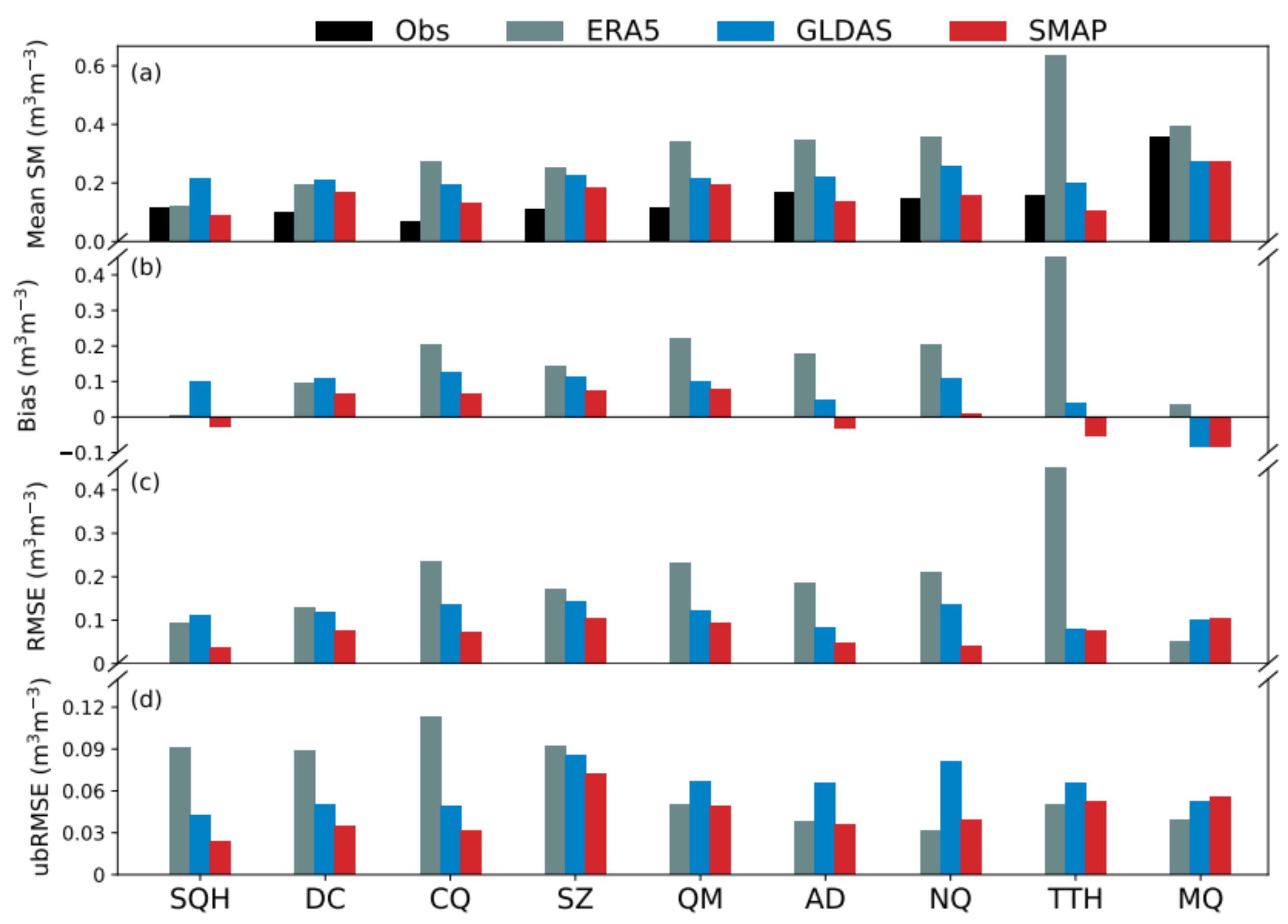
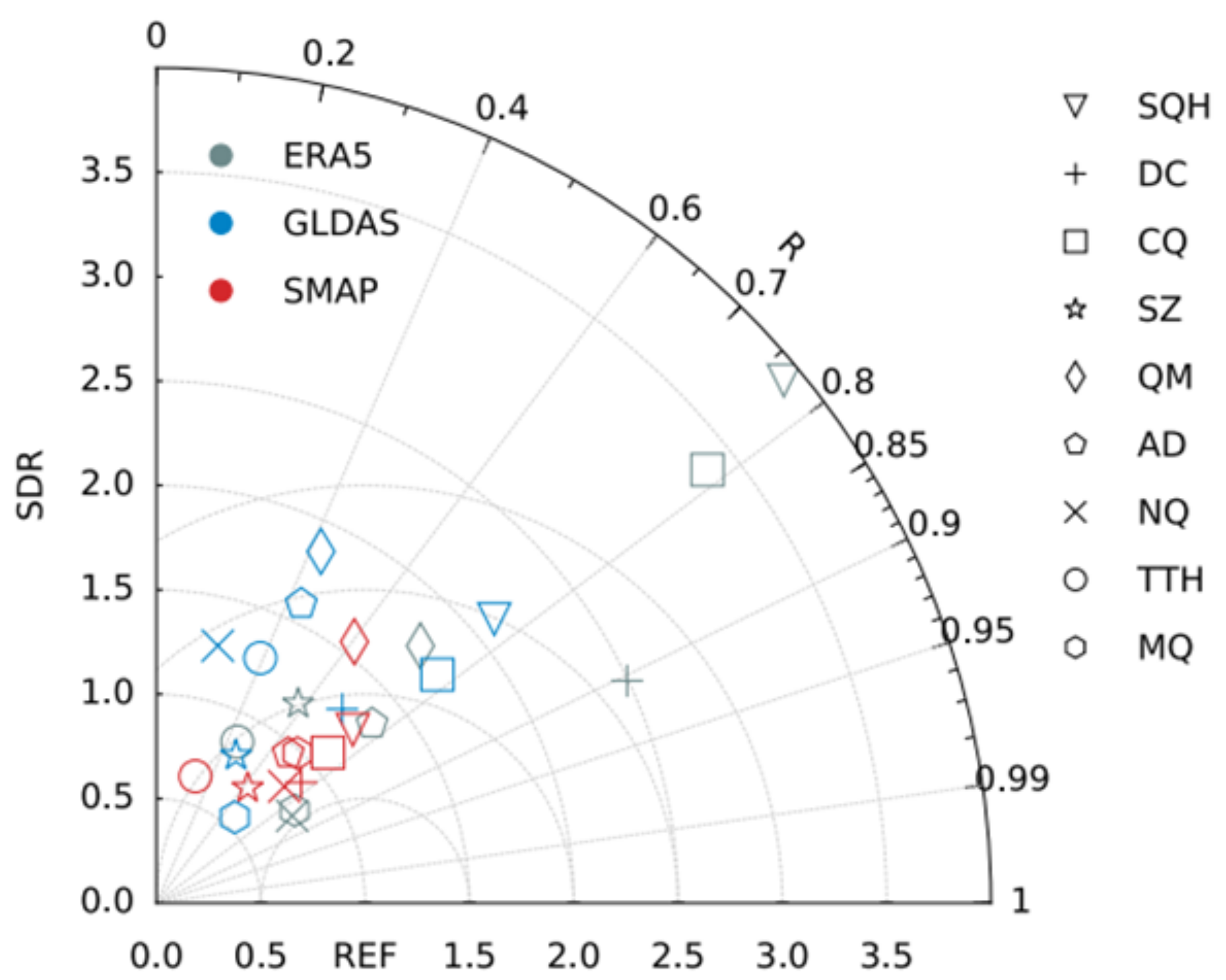
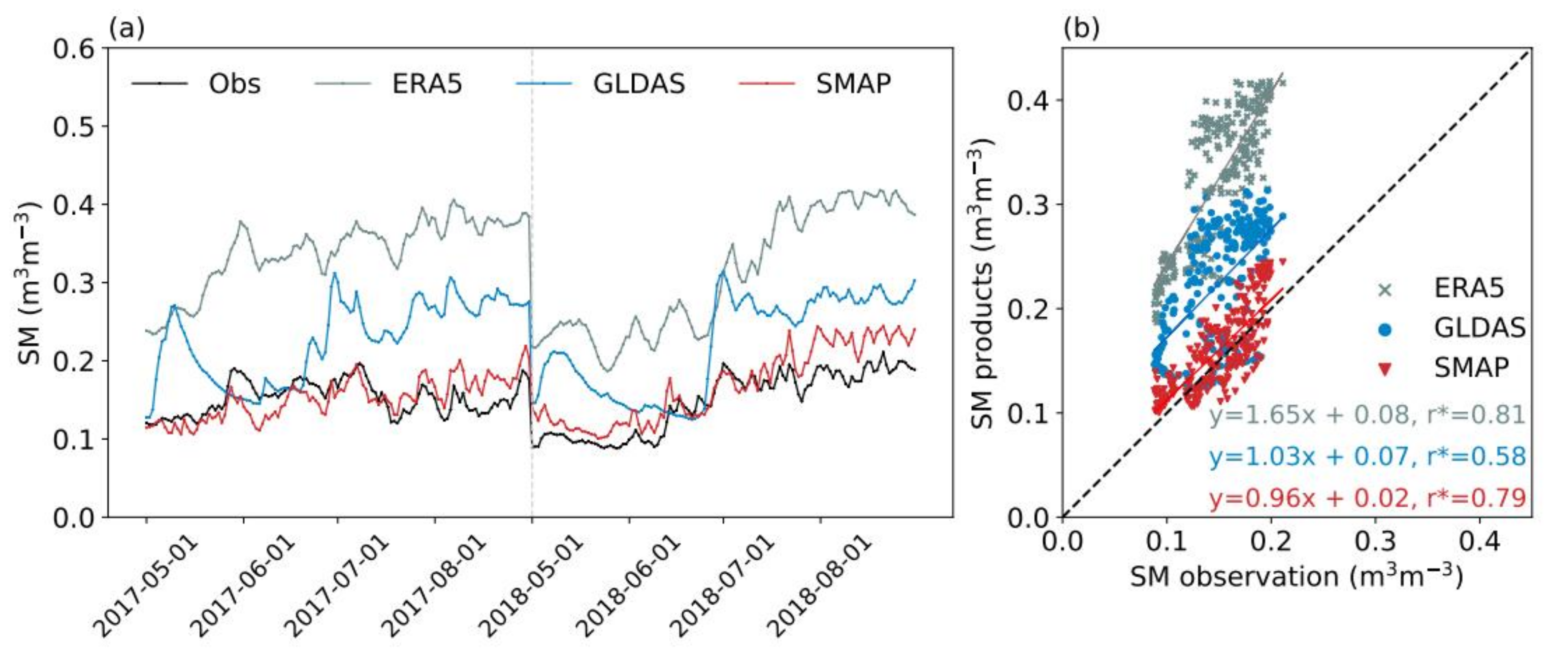
Product evaluation based on In Situ observations indicates that both ERA5 and GLDAS overestimate TP SM. SMAP-derived SM is the closest to observed SM in terms of magnitude. In terms of capturing the temporal variations of SM measured at the stations, the performance of ERA5 and SMAP is superior to that of GLDAS.

(2)

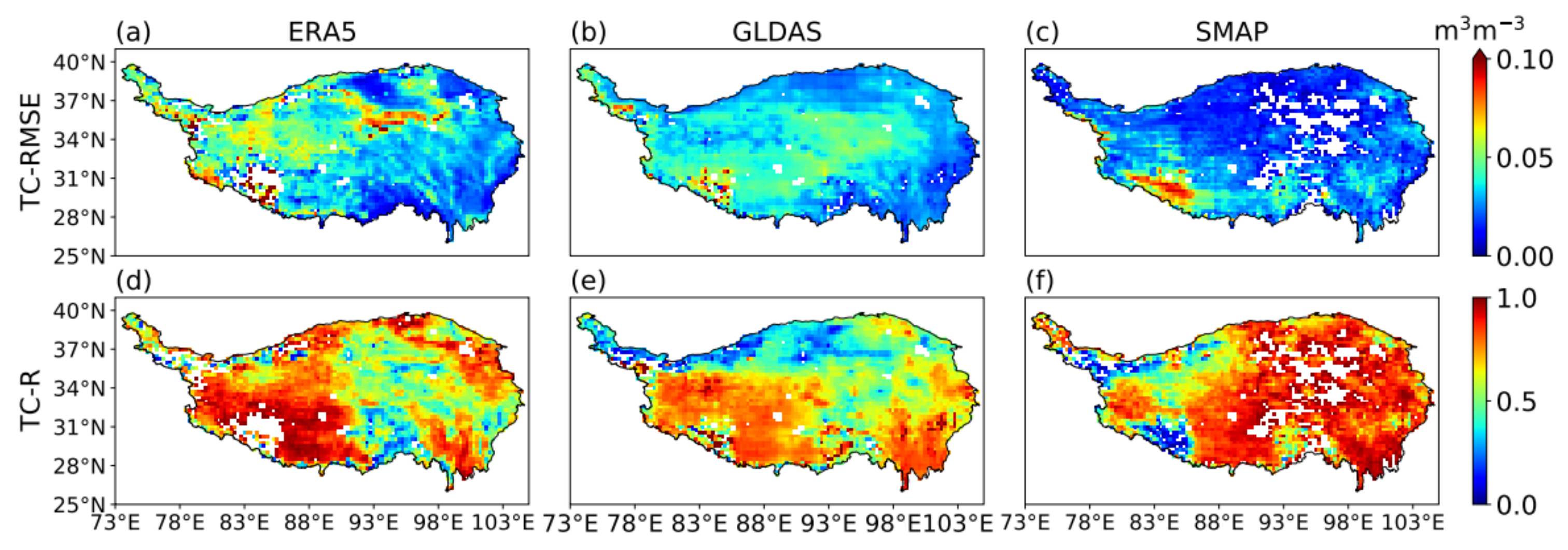
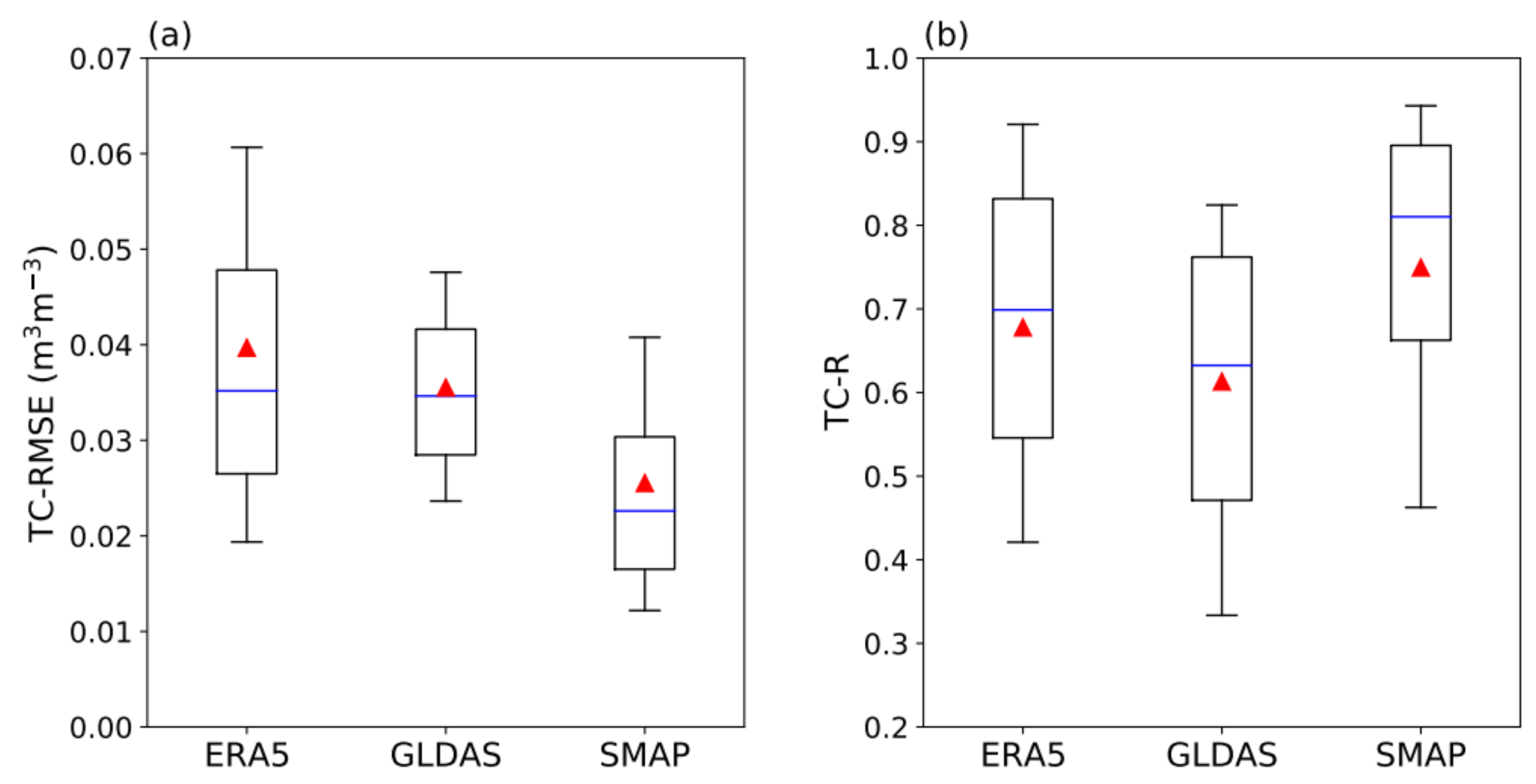
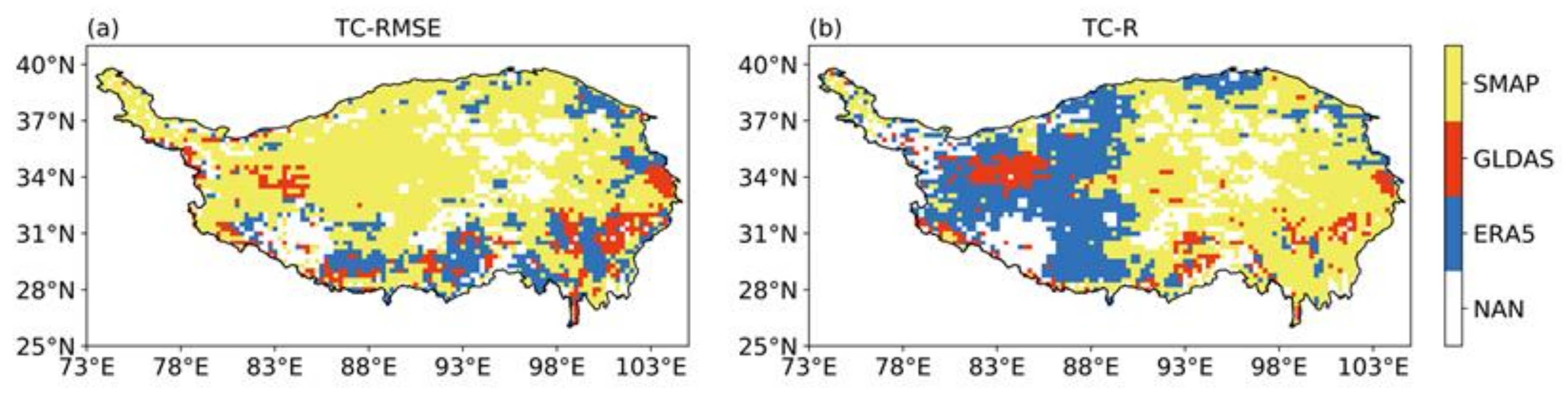
Product evaluation based on TC indicates that the random errors of ERA5 are the largest and those of SMAP are the smallest over the entire TP. Correlation between ERA5-derived SM and the unknown true SM is strong in western TP. For GLDAS, random errors are large and the correlation with true SM is low. In eastern TP, the performance of SMAP is superior to that of ERA5 and GLDAS in terms of correlation with the true SM. In general, results of the evaluation based on TC are consistent with those based on In Situ observations.

(3)

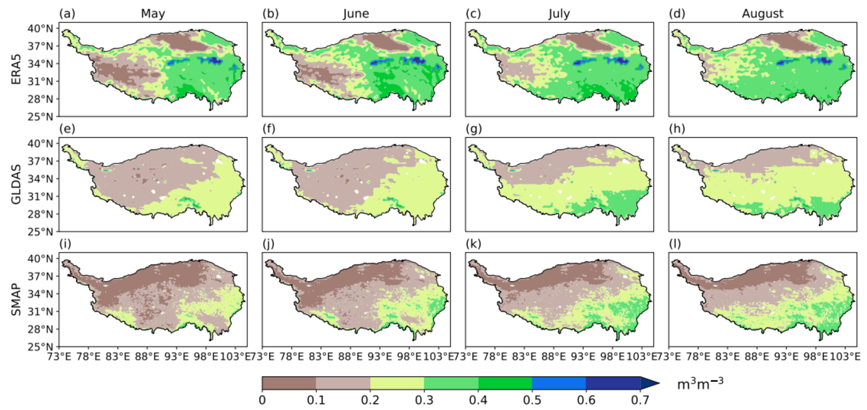
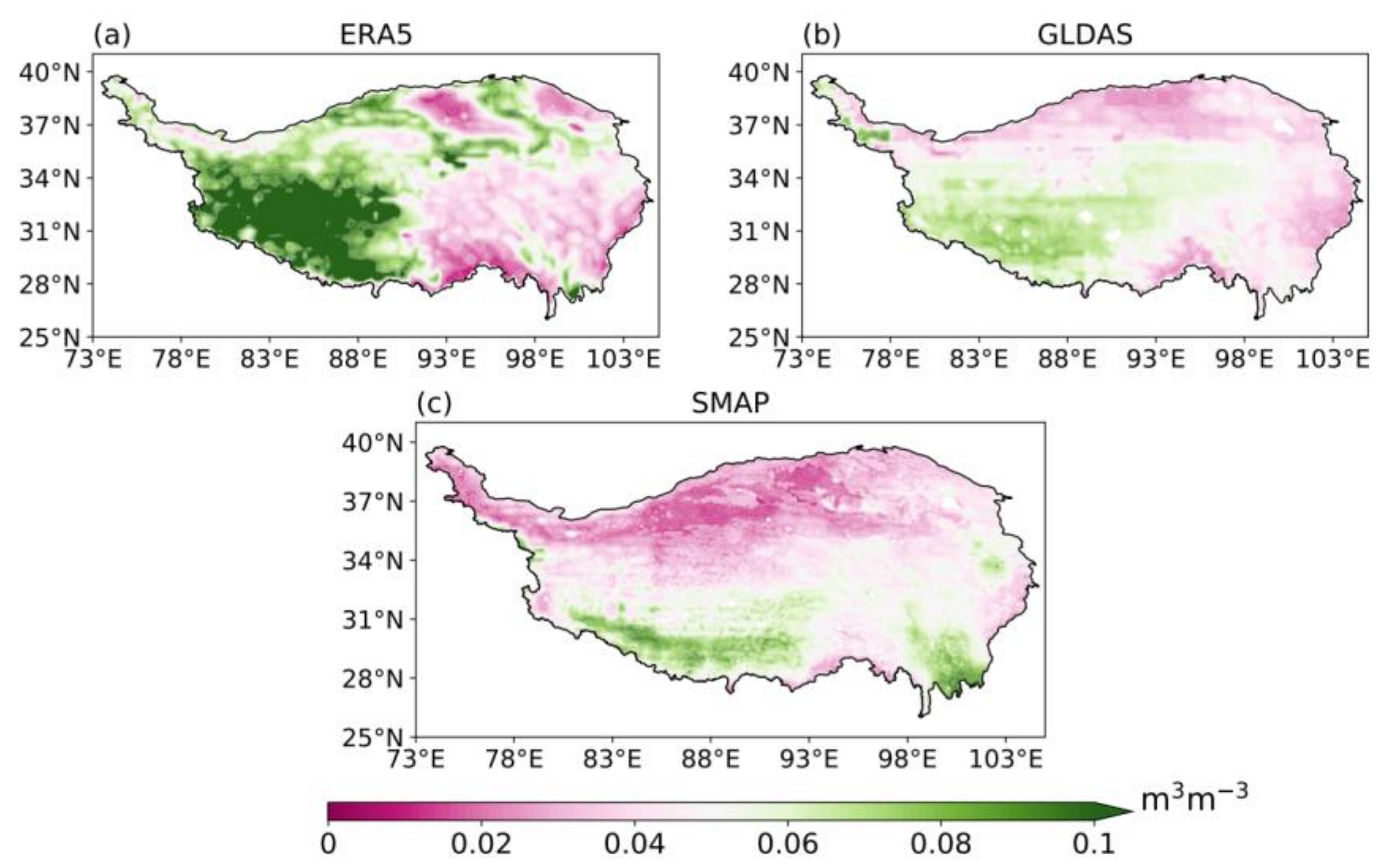
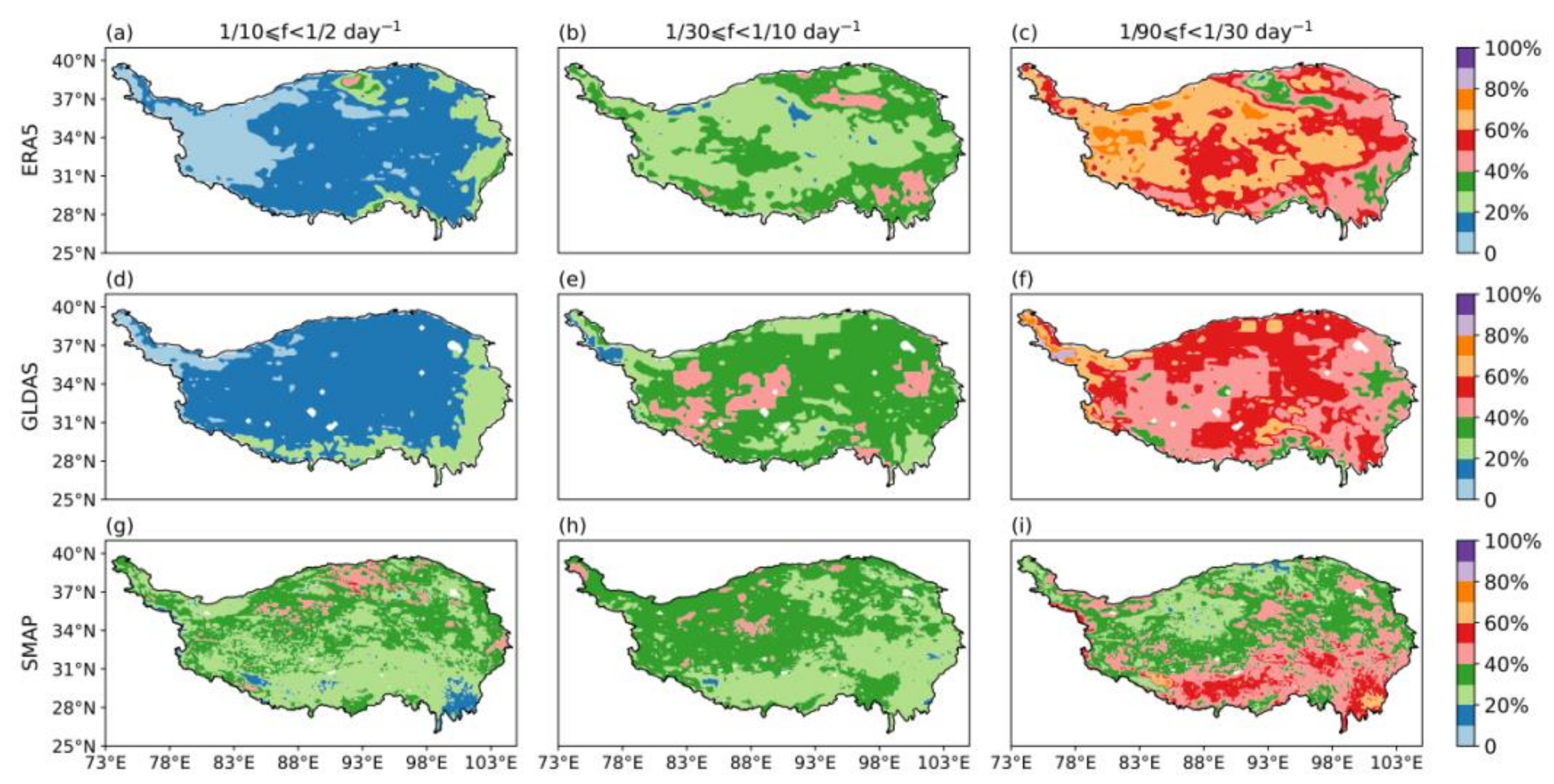
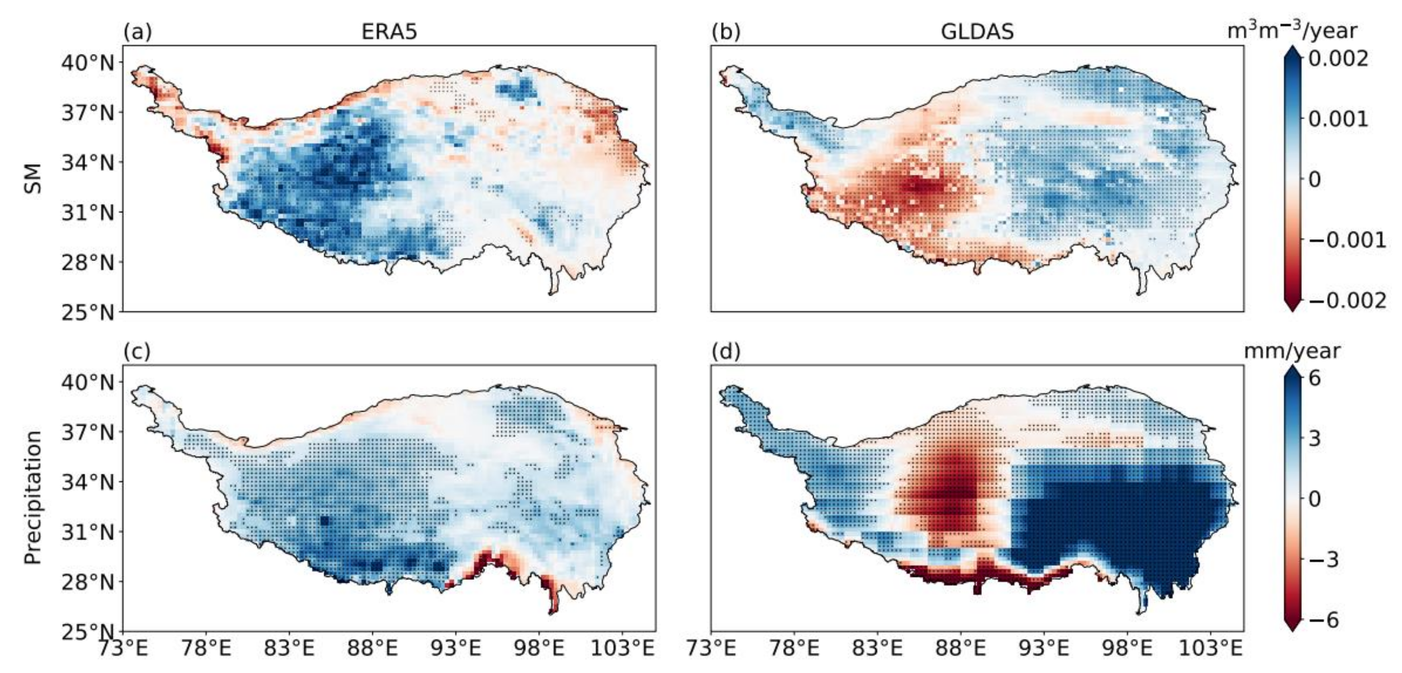
All three products indicate high SM in the southeast, which decreases gradually across the TP towards the northwest. For SMAP, SM variability is the largest in southern TP. For ERA5 and GLDAS and relative to SMAP, SM variability in western TP is high and contribution of high frequencies is low. Intraseasonal variability is the highest on the 30- to 90-day scale. ERA5 performs better than GLDAS in presenting the long-term trends of SM in 1981–2021 over the TP.

(4)

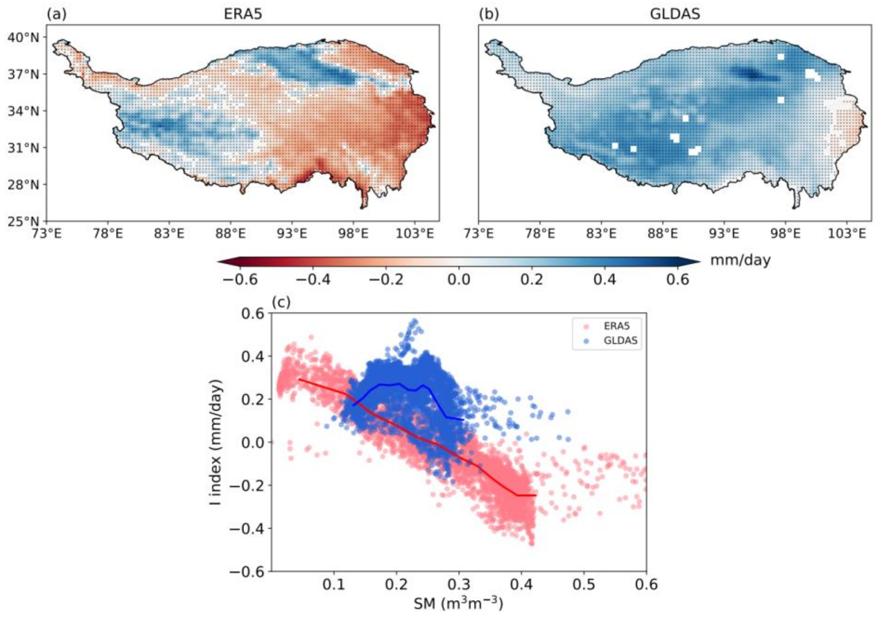
For both ERA5 and GLDAS, land–atmosphere coupling is stronger in western TP, which is relatively dry. Coupling is weaker in eastern TP, especially for ERA5. This is because SM from ERA5 is considerably higher than that from GLDAS in eastern TP.

In this study, we evaluated the performance of the ERA5, GLDAS, and SMAP SM products over the TP. The results may facilitate the use of these products for disaster monitoring and climate and hydrological studies.

References

1. Robinson, D.A.; Campbell, C.S.; Hopmans, J.W.; Hornbuckle, B.K.; Jones, S.B.; Knight, R.; Ogden, F.; Selker, J.; Wendroth, O. Soil Moisture Measurement for Ecological and Hydrological Watershed-Scale Observatories: A Review. Vadose Zone J. 2008, 7, 358–389. [Google Scholar] [CrossRef] [Green Version]
2. Seneviratne, S.I.; Corti, T.; Davin, E.L.; Hirschi, M.; Jaeger, E.B.; Lehner, I.; Orlowsky, B.; Teuling, A.J. Investigating Soil Moisture–Climate Interactions in a Changing Climate: A Review. Earth-Sci. Rev. 2010, 99, 125–161. [Google Scholar] [CrossRef]
3. Entekhabi, D.; Rodriguez-Iturbe, I.; Castelli, F. Mutual Interaction of Soil Moisture State and Atmospheric Processes. J. Hydrol. 1996, 184, 3–17. [Google Scholar] [CrossRef]
4. Rodriguez-Iturbe, I. Ecohydrology: A Hydrologic Perspective of Climate-Soil-Vegetation Dynamies. Water Resour. Res. 2000, 36, 3–9. [Google Scholar] [CrossRef] [Green Version]
5. Babaeian, E.; Sadeghi, M.; Jones, S.B.; Montzka, C.; Vereecken, H.; Tuller, M. Ground, Proximal, and Satellite Remote Sensing of Soil Moisture. Rev. Geophys. 2019, 57, 530–616. [Google Scholar] [CrossRef] [Green Version]
6. McColl, K.A.; Alemohammad, S.H.; Akbar, R.; Konings, A.G.; Yueh, S.; Entekhabi, D. The Global Distribution and Dynamics of Surface Soil Moisture. Nat. Geosci. 2017, 10, 100–104. [Google Scholar] [CrossRef]
7. Koster, R.D.; Dirmeyer, P.A.; Guo, Z.; Bonan, G.; Chan, E.; Cox, P. Regions of Strong Coupling Between Soil Moisture and Precipitation. Science 2004, 305, 1138–1140. [Google Scholar] [CrossRef] [Green Version]
8. Hirschi, M.; Seneviratne, S.I.; Alexandrov, V.; Boberg, F.; Boroneant, C.; Christensen, O.B.; Formayer, H.; Orlowsky, B.; Stepanek, P. Observational Evidence for Soil-Moisture Impact on Hot Extremes in Southeastern Europe. Nat. Geosci. 2011, 4, 17–21. [Google Scholar] [CrossRef]
9. Massari, C.; Brocca, L.; Moramarco, T.; Tramblay, Y.; Didon Lescot, J.-F. Potential of Soil Moisture Observations in Flood Modelling: Estimating Initial Conditions and Correcting Rainfall. Adv. Water Resour. 2014, 74, 44–53. [Google Scholar] [CrossRef]
10. Rosenzweig, C.; Tubiello, F.N.; Goldberg, R.; Mills, E.; Bloomfield, J. Increased Crop Damage in the US from Excess Precipitation under Climate Change. Glob. Environ. Change 2002, 12, 197–202. [Google Scholar] [CrossRef]
11. Ines, A.V.M.; Das, N.N.; Hansen, J.W.; Njoku, E.G. Assimilation of Remotely Sensed Soil Moisture and Vegetation with a Crop Simulation Model for Maize Yield Prediction. Remote Sens. Environ. 2013, 138, 149–164. [Google Scholar] [CrossRef] [Green Version]
12. Alamilla-Magaña, J.C.; Carrillo-Ávila, E.; Obrador-Olán, J.J.; Landeros-Sánchez, C.; Vera-Lopez, J.; Juárez-López, J.F. Soil Moisture Tension Effect on Sugar Cane Growth and Yield. Agric. Water Manag. 2016, 177, 264–273. [Google Scholar] [CrossRef]
13. Qiu, J. China: The Third Pole. Nature 2008, 454, 393–396. [Google Scholar] [CrossRef] [Green Version]
14. Lu, C.; Yu, G.; Xie, G. Tibetan Plateau Serves as a Water Tower. In Proceedings of the 2005 IEEE International Geoscience and Remote Sensing Symposium, IGARSS ’05, Seoul, Republic of Korea, 25–29 July 2005; Volume 5, pp. 3120–3123. [Google Scholar]
15. Wu, G.; Zhang, Y. Tibetan Plateau Forcing and the Timing of the Monsoon Onset over South Asia and the South China Sea. Mon. Weather Rev. 1998, 126, 913–927. [Google Scholar] [CrossRef]
16. Duan, A.; Hu, J.; Xiao, Z. The Tibetan Plateau Summer Monsoon in the CMIP5 Simulations. J. Clim. 2013, 26, 7747–7766. [Google Scholar] [CrossRef]
17. Ma, Y.; Hu, Z.; Tian, L.; Zhang, F.; Duan, A.; Yang, K.; Zhang, Y.L.; Yang, Y. Study Process of the Tibet Plateau Climate System Change and Mechanism of Its Impact on East Asia. Adv. Earth Sci 2014, 29, 207–215. [Google Scholar]
18. Zhang, D.; Huang, J.; Guan, X.; Chen, B.; Zhang, L. Long-Term Trends of Precipitable Water and Precipitation over the Tibetan Plateau Derived from Satellite and Surface Measurements. J. Quant. Spectrosc. Radiat. Transf. 2013, 122, 64–71. [Google Scholar] [CrossRef]
19. Kuang, X.; Jiao, J.J. Review on Climate Change on the Tibetan Plateau during the Last Half Century. J. Geophys. Res. Atmos. 2016, 121, 3979–4007. [Google Scholar] [CrossRef] [Green Version]
20. You, Q.; Min, J.; Jiao, Y.; Sillanpää, M.; Kang, S. Observed Trend of Diurnal Temperature Range in the Tibetan Plateau in Recent Decades. Int. J. Climatol. 2016, 36, 2633–2643. [Google Scholar] [CrossRef]
21. Deng, M.; Meng, X. Analysis on Soil Moisture Characteristics of Tibetan Plateau Based on GLDAS. J. Arid Meteorol. 2018, 36, 595–602. [Google Scholar]
22. Wan, G.; Yang, M.; Wang, X.; Chen, X. Variations in Soil Moisture at Different Time Scales of BJ Site on the Central Tibetan Plateau. Chinese J. Soil Sci. 2012, 43, 107–115. [Google Scholar] [CrossRef]
23. Su, Z.; De Rosnay, P.; Wen, J.; Wang, L.; Zeng, Y. Evaluation of ECMWF’s Soil Moisture Analyses Using Observations on the Tibetan Plateau. J. Geophys. Res. Atmos. 2013, 118, 5304–5318. [Google Scholar] [CrossRef]
24. Chen, Y.; Yang, K.; Qin, J.; Zhao, L.; Tang, W. Evaluation of AMSR-E Retrievals and GLDAS Simulations against Observations of a Soil Moisture Network on the Central Tibetan Plateau. J. Geophys. Res. Atmos. 2013, 118, 4466–4475. [Google Scholar] [CrossRef]
25. Chen, Y.; Yang, K.; Qin, J.; Cui, Q.; Lu, H.; La, Z.; Han, M.; Tang, W. Evaluation of SMAP, SMOS, and AMSR2 Soil Moisture Retrievals against Observations from Two Networks on the Tibetan Plateau. J. Geophys. Res. 2017, 122, 5780–5792. [Google Scholar] [CrossRef]
26. Zeng, J.; Li, Z.; Chen, Q.; Bi, H.; Qiu, J.; Zou, P. Evaluation of Remotely Sensed and Reanalysis Soil Moisture Products over the Tibetan Plateau Using In-Situ Observations. Remote Sens. Environ. 2015, 163, 91–110. [Google Scholar] [CrossRef]
27. Crow, W.T.; Berg, A.A.; Cosh, M.H.; Loew, A.; Mohanty, B.P.; Panciera, R.; de Rosnay, P.; Ryu, D.; Walker, J.P. Upscaling Sparse Ground-Based Soil Moisture Observations for the Validation of Coarse-Resolution Satellite Soil Moisture Products. Rev. Geophys. 2012, 50, 372. [Google Scholar] [CrossRef] [Green Version]
28. Xu, L.; Chen, N.; Zhang, X.; Moradkhani, H.; Zhang, C.; Hu, C. In-Situ and Triple-Collocation Based Evaluations of Eight Global Root Zone Soil Moisture Products. Remote Sens. Environ. 2021, 254, 112248. [Google Scholar] [CrossRef]
29. Stoffelen, A. Toward the True Near-Surface Wind Speed: Error Modeling and Calibration Using Triple Collocation. J. Geophys. Res. Ocean. 1998, 103, 7755–7766. [Google Scholar] [CrossRef]
30. Dorigo, W.A.; Scipal, K.; Parinussa, R.M.; Liu, Y.Y.; Wagner, W.; de Jeu, R.A.M.; Naeimi, V. Error Characterisation of Global Active and Passive Microwave Soil Moisture Datasets. Hydrol. Earth Syst. Sci. 2010, 14, 2605–2616. [Google Scholar] [CrossRef] [Green Version]
31. Miyaoka, K.; Gruber, A.; Ticconi, F.; Hahn, S.; Wagner, W.; Figa-Saldaña, J.; Anderson, C. Triple Collocation Analysis of Soil Moisture from Metop-A ASCAT and SMOS Against JRA-55 and ERA-Interim. IEEE J. Sel. Top. Appl. Earth Obs. Remote Sens. 2017, 10, 2274–2284. [Google Scholar] [CrossRef]
32. Gruber, A.; Su, C.-H.; Zwieback, S.; Crow, W.; Dorigo, W.; Wagner, W. Recent Advances in (Soil Moisture) Triple Collocation Analysis. Int. J. Appl. Earth Obs. Geoinf. 2016, 45, 200–211. [Google Scholar] [CrossRef]
33. McColl, K.A.; Vogelzang, J.; Konings, A.G.; Entekhabi, D.; Piles, M.; Stoffelen, A. Extended Triple Collocation: Estimating Errors and Correlation Coefficients with Respect to an Unknown Target. Geophys. Res. Lett. 2014, 41, 6229–6236. [Google Scholar] [CrossRef]
34. Zhao, P.; Xu, X.; Chen, F.; Guo, X.; Zheng, X.; Liu, L.; Hong, Y.; Li, Y.; La, Z.; Peng, H.; et al. The Third Atmospheric Scientific Experiment for Understanding the Earth–Atmosphere Coupled System over the Tibetan Plateau and Its Effects. Bull. Am. Meteorol. Soc. 2018, 99, 757–776. [Google Scholar] [CrossRef]
35. Qiu, J.; Crow, W.T.; Nearing, G.S. The Impact of Vertical Measurement Depth on the Information Content of Soil Moisture for Latent Heat Flux Estimation. J. Hydrometeorol. 2016, 17, 2419–2430. [Google Scholar] [CrossRef]
36. Yang, J.; Huang, X. The 30 m annual land cover dataset and its dynamics in China from 1990 to 2019. Earth System Science Data. 2021, 13, 3907–3925. [Google Scholar] [CrossRef]
37. Hersbach, H.; Bell, B.; Berrisford, P.; Hirahara, S.; Horányi, A.; Muñoz-Sabater, J.; Nicolas, J.; Peubey, C.; Radu, R.; Schepers, D.; et al. The ERA5 Global Reanalysis. Q. J. R. Meteorol. Soc. 2020, 146, 1999–2049. [Google Scholar] [CrossRef]
38. Ling, X.; Huang, Y.; Guo, W.; Wang, Y.; Chen, C.; Qiu, B.; Ge, J.; Qin, K.; Xue, Y.; Peng, J. Comprehensive Evaluation of Satellite-Based and Reanalysis Soil Moisture Products Using in Situ Observations over China. Hydrol. Earth Syst. Sci. 2021, 25, 4209–4229. [Google Scholar] [CrossRef]
39. Deng, M.; Meng, X.; Li, Z.; Lyv, Y.; Lei, H.; Zhao, L.; Zhao, S.; Ge, J.; Jing, H. Responses of Soil Moisture to Regional Climate Change over the Three Rivers Source Region on the Tibetan Plateau. Int. J. Climatol. 2020, 40, 2403–2417. [Google Scholar] [CrossRef]
40. Rodell, M.; Houser, P.R.; Jambor, U.; Gottschalck, J.; Mitchell, K.; Meng, C.J.; Arsenault, K.; Cosgrove, B.; Radakovich, J.; Bosilovich, M.; et al. The Global Land Data Assimilation System. Bull. Am. Meteorol. Soc. 2004, 85, 381–394. [Google Scholar] [CrossRef] [Green Version]
41. Chen, F.; Crow, W.T.; Bindlish, R.; Colliander, A.; Burgin, M.S.; Asanuma, J.; Aida, K. Global-Scale Evaluation of SMAP, SMOS and ASCAT Soil Moisture Products Using Triple Collocation. Remote Sens. Environ. 2018, 214, 1–13. [Google Scholar] [CrossRef]
42. Brown, M.E.; Escobar, V.; Moran, S.; Entekhabi, D.; O’Neill, P.E.; Njoku, E.G.; Doorn, B.; Entin, J.K. NASA’s Soil Moisture Active Passive (SMAP) Mission and Opportunities for Applications Users. Bull. Am. Meteorol. Soc. 2013, 94, 1125–1128. [Google Scholar] [CrossRef]
43. Reichle, R.H.; De Lannoy, G.J.M.; Liu, Q.; Ardizzone, J.V.; Colliander, A.; Conaty, A.; Crow, W.; Jackson, T.J.; Jones, L.A.; Kimball, J.S.; et al. Assessment of the SMAP Level-4 Surface and Root-Zone Soil Moisture Product Using in Situ Measurements. J. Hydrometeorol. 2017, 18, 2621–2645. [Google Scholar] [CrossRef]
44. Reichle, R.; De Lannoy, G.; Koster, R.D.; Crow, W.T.; Jees, S.; Kimball, Q.L. SMAP L4 Global 9 km EASE-Grid Surface and Root Zone Soil Moisture Land Model Constants; Version 6; (SPL4SMLM) [Surface Soil Moisture]; National Snow and Ice Data Center: Boulder, CO, USA, 2021. [Google Scholar]
45. Ding, X.; Lan, X.; Fan, G. Analysis on the Applicability of Reanalysis Soil Temperature and Moisture Datasets over Qinghai—Tibetan Platea. Plateau Meteorol. 2018, 37, 626–641. [Google Scholar] [CrossRef]
46. Montzka, C.; Cosh, M.; Bayat, B.; Al Bitar, A.; Berg, A.; Bindlish, R.; Bogena, H.R.; Bolten, J.D.; Cabot, F.; Caldwell, T. Soil Moisture Product Validation Good Practices Protocol Version 1.0. Good Pract. Satell. Deriv. L. Prod. Valid. 2021, 123, 187. [Google Scholar]
47. Gupta, H.V.; Kling, H.; Yilmaz, K.K.; Martinez, G.F. Decomposition of the Mean Squared Error and NSE Performance Criteria: Implications for Improving Hydrological Modelling. J. Hydrol. 2009, 377, 80–91. [Google Scholar] [CrossRef] [Green Version]
48. Ruane, A.C.; Roads, J.O. 6-Hour to 1-Year Variance of Five Global Precipitation Sets. Earth Interact. 2007, 11, 1–29. [Google Scholar] [CrossRef]
49. Wei, J.; Dirmeyer, P.A.; Guo, Z. How Much Do Different Land Models Matter for Climate Simulation? Part II: A Decomposed View of the Land-Atmosphere Coupling Strength. J. Clim. 2010, 23, 3135–3145. [Google Scholar] [CrossRef]
50. Xi, X.; Gentine, P.; Zhuang, Q.; Kim, S. Evaluating the Variability of Surface Soil Moisture Simulated within CMIP5 Using SMAP Data. J. Geophys. Res. Atmos. 2022, 127, e2021JD035363. [Google Scholar] [CrossRef]
51. Santanello, J.A.; Dirmeyer, P.A.; Ferguson, C.R.; Findell, K.L.; Tawfik, A.B.; Berg, A.; Ek, M.; Gentine, P.; Guillod, B.P.; Van Heerwaarden, C.; et al. Land-Atmosphere Interactions the LoCo Perspective. Bull. Am. Meteorol. Soc. 2018, 99, 1253–1272. [Google Scholar] [CrossRef]
52. Dirmeyer, P.A. The Terrestrial Segment of Soil Moisture–Climate Coupling. Geophys. Res. Lett. 2011, 38, 2754. [Google Scholar] [CrossRef]
53. Meng, X.; Li, R.; Luan, L.; Lyu, S.; Zhang, T.; Ao, Y.; Han, B.; Zhao, L.; Ma, Y. Detecting Hydrological Consistency between Soil Moisture and Precipitation and Changes of Soil Moisture in Summer over the Tibetan Plateau. Clim. Dyn. 2018, 51, 4157–4168. [Google Scholar] [CrossRef] [Green Version]
54. Zhong, L.; Ma, Y.; Salama, M.S.; Su, Z. Assessment of Vegetation Dynamics and Their Response to Variations in Precipitation and Temperature in the Tibetan Plateau. Clim. Change 2010, 103, 519–535. [Google Scholar] [CrossRef]
55. Bengtsson, L. The Global Atmospheric Water Cycle. Environ. Res. Lett. 2010, 5, 25202. [Google Scholar] [CrossRef]
56. Sun, J.; Yang, K.; Guo, W.; Wang, Y.; He, J.; Lu, H. Why Has the Inner Tibetan Plateau Become Wetter since the Mid-1990s? J. Clim. 2020, 33, 8507–8522. [Google Scholar] [CrossRef]
57. Yao, T.; Bolch, T.; Chen, D.; Gao, J.; Imerzeel, W.; Piao, S.; Su, F.; Thompson, L.; Wada, Y.; Wang, L.; et al. The imbalance of the Asian water tower. Nat. Rev. Earth Environ. 2022, 3, 618–632. [Google Scholar] [CrossRef]
58. Lai, H.W.; Chen, H.W.; Kukulies, J.; Ou, T.; Chen, D. Regionalization of Seasonal Precipitation over the Tibetan Plateau and Associated Large-Scale Atmospheric Systems. J. Clim. 2021, 34, 2635–2651. [Google Scholar] [CrossRef]
59. Wei, J.; Dirmeyer, P.A. Dissecting Soil Moisture-Precipitation Coupling. Geophys. Res. Lett. 2012, 39, L19711. [Google Scholar] [CrossRef]
60. Li, C.; Lu, H.; Yang, K.; Han, M.; Wright, J.S.; Chen, Y.; Yu, L.; Xu, S.; Huang, X.; Gong, W. The Evaluation of SMAP Enhanced Soil Moisture Products Using High-Resolution Model Simulations and In-Situ Observations on the Tibetan Plateau. Remote Sens. 2018, 10, 535. [Google Scholar] [CrossRef] [Green Version]
61. Liu, J.; Chai, L.; Lu, Z.; Liu, S.; Qu, Y.; Geng, D.; Song, Y.; Guan, Y.; Guo, Z.; Wang, J.; et al. Evaluation of SMAP, SMOS-IC, FY3B, JAXA, and LPRM Soil Moisture Products over the Qinghai-Tibet Plateau and Its Surrounding Areas. Remote Sens. 2019, 11, 792. [Google Scholar] [CrossRef] [Green Version]
62. Xing, Z.; Fan, L.; Zhao, L.; De Lannoy, G.; Frappart, F.; Peng, J.; Li, X.; Zeng, J.; Al-Yaari, A.; Yang, K.; et al. A First Assessment of Satellite and Reanalysis Estimates of Surface and Root-Zone Soil Moisture over the Permafrost Region of Qinghai-Tibet Plateau. Remote Sens. Environ. 2021, 265, 112666. [Google Scholar] [CrossRef]
63. Yang, S.; Li, R.; Wu, T.; Hu, G.; Xiao, Y.; Du, Y.; Zhu, X.; Ni, J.; Ma, J.; Zhang, Y.; et al. Evaluation of Reanalysis Soil Temperature and Soil Moisture Products in Permafrost Regions on the Qinghai-Tibetan Plateau. Geoderma 2020, 377, 114583. [Google Scholar] [CrossRef]
64. Derber, J.C.; Parrish, D.F.; Lord, S.J. The New Global Operational Analysis System at the National Meteorological Center. Weather Forecast 1991, 6, 538–547. [Google Scholar] [CrossRef]
65. Adler, R.F.; Huffman, G.J.; Chang, A.; Ferraro, R.; Xie, P.-P.; Janowiak, J.; Rudolf, B.; Schneider, U.; Curtis, S.; Bolvin, D.; et al. The Version-2 Global Precipitation Climatology Project (GPCP) Monthly Precipitation Analysis (1979–Present). J. Hydrometeorol. 2003, 4, 1147–1167. [Google Scholar] [CrossRef]
66. Qin, Y.; Wu, T.; Wu, X.; Li, R.; Xie, C.; Qiao, Y.; Hu, G.; Zhu, X.; Wang, W.; Shang, W. Assessment of Reanalysis Soil Moisture Products in the Permafrost Regions of the Central of the Qinghai–Tibet Plateau. Hydrol. Process. 2017, 31, 4647–4659. [Google Scholar] [CrossRef]
67. Deng, K.A.K.; Lamine, S.; Pavlides, A.; Petropoulos, G.P.; Bao, Y.; Srivastava, P.K.; Guan, Y. Large Scale Operational Soil Moisture Mapping from Passive MW Radiometry: SMOS Product Evaluation in Europe & USA. Int. J. Appl. Earth Obs. Geoinf. 2019, 80, 206–217. [Google Scholar] [CrossRef]
68. Liu, J.; Chai, L.; Dong, J.; Zheng, D.; Wigneron, J.-P.; Liu, S.; Zhou, J.; Xu, T.; Yang, S.; Song, Y.; et al. Uncertainty Analysis of Eleven Multisource Soil Moisture Products in the Third Pole Environment Based on the Three-Corned Hat Method. Remote Sens. Environ. 2021, 255, 112225. [Google Scholar] [CrossRef]
69. Zhao, T.; Shi, J.; Entekhabi, D.; Jackson, T.J.; Hu, L.; Peng, Z.; Yao, P.; Li, S.; Kang, C.S. Retrievals of Soil Moisture and Vegetation Optical Depth Using a Multi-Channel Collaborative Algorithm. Remote Sens. Environ. 2021, 257, 112321. [Google Scholar] [CrossRef]
70. Hu, F.; Wei, Z.; Yang, X.; Xie, W.; Li, Y.; Cui, C.; Yang, B.; Tao, C.; Zhang, W.; Meng, L. Assessment of SMAP and SMOS Soil Moisture Products Using Triple Collocation Method over Inner Mongolia. J. Hydrol. Reg. Stud. 2022, 40, 101027. [Google Scholar] [CrossRef]
71. Piepmeier, J.R.; Johnson, J.T.; Mohammed, P.N.; Bradley, D.; Ruf, C.; Aksoy, M.; Garcia, R.; Hudson, D.; Miles, L.; Wong, M. Radio-Frequency Interference Mitigation for the Soil Moisture Active Passive Microwave Radiometer. IEEE Trans. Geosci. Remote Sens. 2014, 52, 761–775. [Google Scholar] [CrossRef]
Figure 1. Spatial distribution of (a) topographic height, (b) land cover and (c) soil sand percentage. Black dots present the nine observation stations on the Tibetan Plateau (TP): Shiquanhe (SQH), Dongcuo (DC), Cuoqin (CQ), Shenzha (SZ), Qiangma (QM), Anduo (AD), Naqu (NQ), Tuotuohe (TTH), and Maqu (MQ). The 30 m resolution land cover in (b) is obtained from the Earth System Science Data [36]. The soil sand content data in (c) is from Resources and Environmental Sciences, Chinese Academy of Sciences (RESDC) (http://www.resdc.cn (accessed on 1 January 2022)).
Remotesensing 14 05819 g001
Figure 2. The (a) climatology, (b) mean bias (Bias), (c) root mean square error (RMSE), and (d) unbiased RMSE (ubRMSE) of product-derived soil moisture (SM) relative to In Situ measurements of SM for May to August in 2017 and 2018 on the Tibetan Plateau.
Remotesensing 14 05819 g002
Figure 3. Taylor diagram of the Pearson correlation coefficient (R) and the ratio of the standard deviation (SDR) of product-derived soil moisture (SM) relative to In Situ measurements of SM; REF indicates In Situ SM measurements.
Remotesensing 14 05819 g003
Figure 4. Decomposition of the three terms of the mean square error (MSE) for the three soil moisture products at nine observation stations.
Remotesensing 14 05819 g004
Figure 5. Soil moisture (a) time series and (b) scatterplot for three soil moisture products and In Situ observations for May to August in 2017 and 2018. * represents the Pearson correlation coefficient (r) is statistically significant at the 95% confidence level according to Student’s t test.
Remotesensing 14 05819 g005
Figure 6. Spatial distribution of (ac) the standard deviation of random errors derived from triple collocation (TC-RMSE) and (df) triple collocation correlation coefficients (TC-R) for (left column) the fifth-generation European Centre for Medium-Range Weather Forecasts atmospheric reanalysis (ERA5), (central column) Global Land Data Assimilation System (GLDAS), and (right column) Soil Moisture Active Passive (SMAP) datasets.
Remotesensing 14 05819 g006
Figure 7. Boxplots of (a) the standard deviation of random errors derived from triple collocation (TC-RMSE) and (b) triple collocation correlation coefficients (TC-R) for all grids in the three products. Blue line indicates the median. Triangle indicates the mean. Bottom and top horizontal lines indicate the 10% and the 90% quantiles, respectively.
Remotesensing 14 05819 g007
Figure 8. Optimal product with (a) the lowest standard deviation of random errors derived from triple collocation (TC-RMSE) and (b) the highest triple collocation correlation coefficient (TC-R) for each grid cell. Blank indicates missing values due to violation of triple collocation assumptions.
Remotesensing 14 05819 g008
Figure 9. Spatial distribution of monthly average soil moisture derived from (ad) the fifth-generation European Centre for Medium-Range Weather Forecasts atmospheric reanalysis (ERA5), (eh) Global Land Data Assimilation System (GLDAS), and (il) Soil Moisture Active Passive (SMAP) datasets for May to August 2015–2021 over the Tibetan Plateau.
Remotesensing 14 05819 g009
Figure 10. Spatial distribution of the standard deviation of daily soil moisture for May, June, July, and August derived from (a) the fifth-generation European Centre for Medium-Range Weather Forecasts atmospheric reanalysis (ERA5), (b) Global Land Data Assimilation System (GLDAS), and (c) Soil Moisture Active Passive (SMAP) datasets.
Remotesensing 14 05819 g010
Figure 11. Variance percentages of the (left column) high-, (central column) intermediate-, and (right column) low-frequency bands from (ac) the fifth-generation European Centre for Medium-Range Weather Forecasts atmospheric reanalysis (ERA5), (df) Global Land Data Assimilation System (GLDAS), and (gi) Soil Moisture Active Passive (SMAP) datasets.
Remotesensing 14 05819 g011
Figure 12. Annual trends of (a) soil moisture (SM) derived from the fifth-generation European Centre for Medium-Range Weather Forecasts atmospheric reanalysis (ERA5) dataset, (b) SM derived from the Global Land Data Assimilation System (GLDAS) dataset, (c) precipitation derived from ERA5, and (d) precipitation derived from GLDAS for the warm season between 1981 and 2021 over the Tibetan Plateau. Dots indicate areas with trends that are statistically significant at the 95% confidence level according to Student’s t test.
Remotesensing 14 05819 g012
Figure 13. Spatial distribution of the terrestrial coupling index (I) in May, June, July, and August of 1981–2021 derived from soil moisture (SM) and evapotranspiration (ET) from (a) the fifth-generation European Centre for Medium-Range Weather Forecasts atmospheric reanalysis (ERA5) and (b) Global Land Data Assimilation System (GLDAS) datasets. Positive values indicate strong coupling. Dots indicate areas with trends that are statistically significant at the 95% confidence level according to Student’s t tests. (c) Pointwise relationships between I index and SM for ERA5 and GLDAS. The lines are the averages for the points (the points are separated into 13 groups according to the ranking of SM and the averages for the groups are shown).
Remotesensing 14 05819 g013
Publisher’s Note: MDPI stays neutral with regard to jurisdictional claims in published maps and institutional affiliations.