Communication

Quantum Based Pseudo-Labelling for Hyperspectral Imagery: A Simple and Efficient Semi-Supervised Learning Method for Machine Learning Classifiers

1
Super GeoAI Technology Inc., 229-116 Research Drive, Saskatoon, SK S7N 3R3, Canada
2
Department of Mechanical and Aerospace Engineering, University of Rome ‘La Sapienza’, Via Eudossiana 18, 00184 Rome, Italy
*
Author to whom correspondence should be addressed.
Remote Sens. 2022, 14(22), 5774; https://doi.org/10.3390/rs14225774
Submission received: 26 September 2022 / Revised: 10 November 2022 / Accepted: 13 November 2022 / Published: 16 November 2022
(This article belongs to the Collection Feature Paper Special Issue on Forest Remote Sensing)

Abstract

:
A quantum machine is a human-made device whose collective motion follows the laws of quantum mechanics. Quantum machine learning (QML) is machine learning for quantum computers. The availability of quantum processors has led to practical applications of QML algorithms in the remote sensing field. Quantum machines can learn from fewer data than non-quantum machines, but because of their low processing speed, quantum machines cannot be applied to an image that has hundreds of thousands of pixels. Researchers around the world are exploring applications for QML and in this work, it is applied for pseudo-labelling of samples. Here, a PRISMA (PRecursore IperSpettrale della Missione Applicativa) hyperspectral dataset is prepared by quantum-based pseudo-labelling and 11 different machine learning algorithms viz., support vector machine (SVM), K-nearest neighbour (KNN), random forest (RF), light gradient boosting machine (LGBM), XGBoost, support vector classifier (SVC) + decision tree (DT), RF + SVC, RF + DT, XGBoost + SVC, XGBoost + DT, and XGBoost + RF with this dataset are evaluated. An accuracy of 86% was obtained for the classification of pine trees using the hybrid XGBoost + decision tree technique.

1. Introduction

The predictive power of hybrid/deep learning (DL) classifiers makes them the primary option for remote sensing researchers [1]. Annotated datasets are used to develop and evaluate machine learning (ML)/deep learning. However, in remote sensing applications, only a small amount of labelled data is available for training. As labelled data is expensive to collect, abundant unlabelled data are used [2]. Field observations must be conducted across different locations of the studied region to ensure the sampling points have a high spatial variability, similar to that of satellite data acquisition. The accuracy of machine learning techniques depends on the magnitude of the training dataset. For classical ML, large datasets are required to obtain higher accuracy, so annotated datasets are a crucial pre-condition for modelling and validating ML-based classifications. Unfortunately, due to the heterogeneity of remote sensing measurements and tasks, there is no single go-to dataset that can serve as a standardized pre-training benchmark [2]. Therefore, researchers are developing procedures to create datasets on their own in a semi-supervised approach [3]. Pseudo-labelling makes abundant unlabelled data available in the image for training ML models. QML has the ability to learn from smaller datasets using a procedure of pseudo-labelling, i.e., annotating the unlabelled data of a hyperspectral image using a quantum support vector machine (QSVM), which is proposed [4].
QML is an interdisciplinary field of quantum mechanics, and ML outperforms classical computation by outsourcing complex computations to a quantum computer [5]. The performance of QML implemented for big data applications is compared with the performance of classical computation [6,7,8]. Two major providers of cloud QC environments are IBM (gate-based systems) [5,9] and D-Wave (based on quantum annealing) [10,11]. The main goal of many researchers in this field is to search for potential applications that demonstrate quantum speed-ups [6]. Quantum computers can recognize complex patterns of labelled data that are not recognised by classical computers; the latter need more dimensional planes. A quantum support vector machine (QSVM) was chosen in this study because QSVM can be trained with comparatively lesser samples, which attracts most users [12]. Different models look for different trends and patterns. It is tricky to predict which model will perform best before each model is tested. The classification accuracy depends on the size, quality, and nature of the training data; the training time; and the expected results [13,14]. In the present study, different machine learning methods were evaluated, and the parameters were tuned to reach the desired accuracy. Pseudo-labels were assigned to samples of hyperspectral data and 11 different ML techniques were applied to evaluate the quantum-based dataset.
In this short communication, firstly, the procedure of quantum based pseudo-labelling of samples is demonstrated. From the literature [3], it was observed that QSVM has the highest accuracy for hyperspectral classification problems but cannot be used for predicting a large-scale (30 km × 30 km) image because of the limitation on the prediction speed. Since data scarcity is one of the challenges faced by most remote sensing scientists, a quantum-based pseudo-labelling procedure is proposed as a solution to this challenge for pine tree classification. Secondly, different machine learning techniques viz., support vector machine (SVM), K-nearest neighbour (KNN), random forest (RF), light gradient boosting machine (LGBM), XGBoost, support vector classifier (SVC) + decision tree (DT), RF + SVC, RF + DT, XGBoost + SVC, XGBoost + DT, and XGBoost + RF were evaluated and a technique that gives better accuracy with quantum-based pseudo-labelled PRISMA dataset was also found. This manuscript is organized into four sections. Section 2 describes the study area, the reference data, and the PRISMA satellite data used for the analysis. Section 3 presents the methods used. Section 4 explains the experimental setup. Section 5 presents the results and discusses the classifications and the validation information presented. Section 6 explains the conclusions derived from this study.

2. Data and Methods

2.1. Study Area

The hyperspectral PRISMA (PRecursore IperSpettrale della Missione Applicativa) data shown in Figure 1 comprises the estate of Castel Porziano in Rome and was acquired on 27 June 2021. This image was downloaded from the PRISMA archive on https://prisma.asi.it/ (accessed on 15 May 2022). Pine trees cover the majority of this estate. Additionally, this estate has different oak trees, cork trees, shrubs, and grasslands. This region has a humid climate and the temperature in this area varies from −5 °C in winter to 31 °C in summer. The region covered in this image has an elevation varying from 20 to 70 feet.

2.2. Reference Data

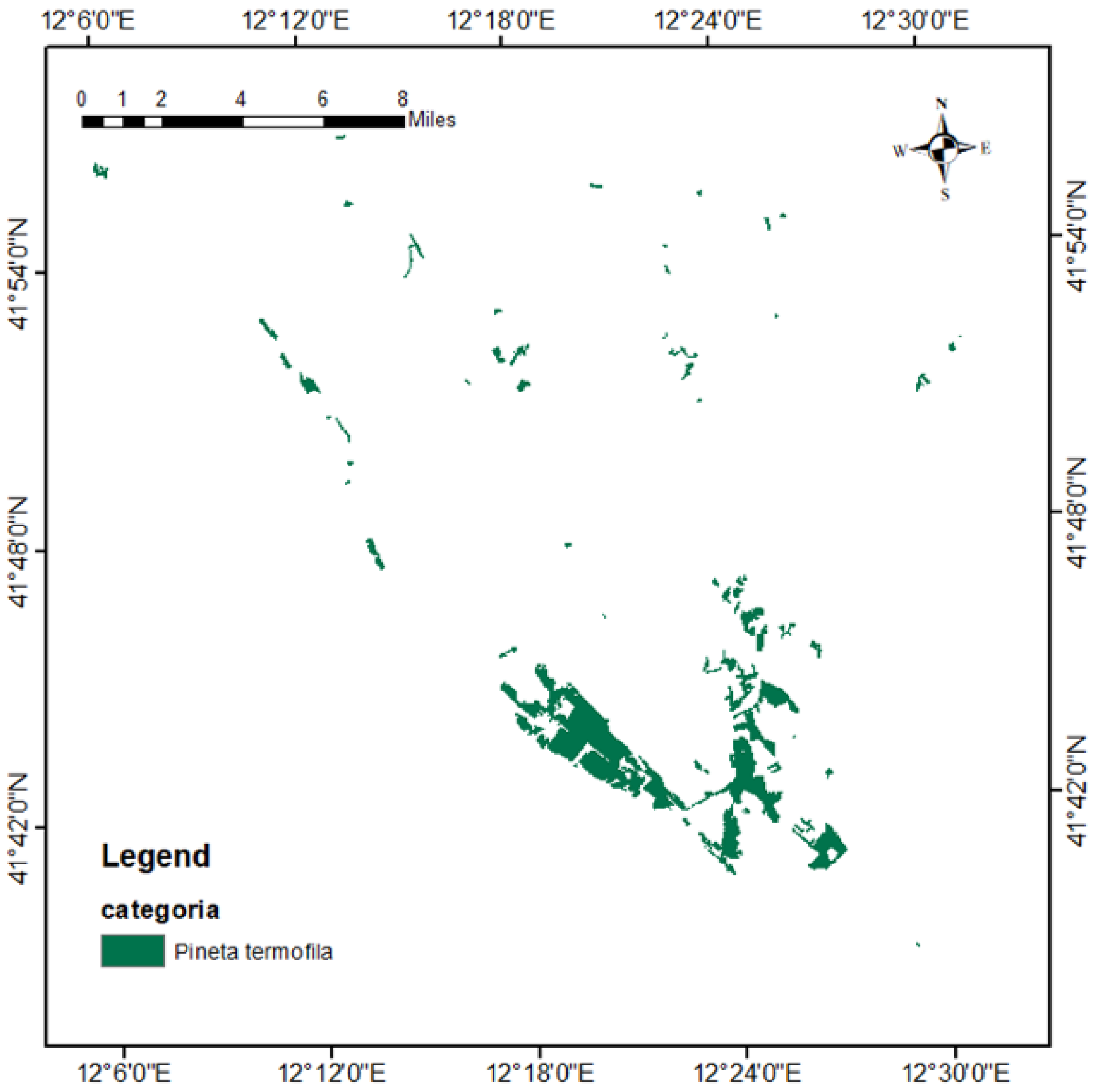
Reference data (Figure 2) were extracted from a ground truth vegetation map (2021) provided by the geoportal of the Lazio regional administration. This data was provided in shapefile format and converted to GTiff on ArcMap, giving a spatial resolution of 30 m. The area shown in green is covered by pine vegetation, which comprised the input for training the ML models.

2.3. Pre-Processing of PRISMA Data

PRISMA, a satellite of the Italian space agency (Agenzia Spaziale Italiana, ASI), carries a hyperspectral sensor that enables hyperspectral imaging [13,14]. Using an imaging spectrometer, this sensor captures imagery with a continuum of spectral bands of 400–2500 nm at a spatial resolution of 30 m. There are 173 bands in the shortwave infrared within a 920–2500 nm range, and 66 bands are in the visible near-infrared portion (400–1010 nm) of the spectrum. The widths and spectral sampling intervals are ≤12 nm. A panchromatic camera that provides a single band (400–700 nm) image at a 5 m spatial resolution is also on-board the ASI’s satellite [15].
The PRISMA archive has Level-1, Level-2B, Level-2C, and Level-2D products among which Level-1’s cloud cover and land cover image and Level-2C’s hypercube were considered for processing. For more details on the level-wise images, please refer to https://prisma.asi.it/ (accessed on 15 May 2022). For the region of interest, images of minimal cloud cover downloaded from the archive and remaining clouded pixels were masked using the cloud cover image. Level-1’s land cover image was considered for masking the non-vegetated areas in the hypercube. The Prismaread tool from CNR, Italy (https://irea-cnr-mi.github.io/prismaread/) was accessed on 25 May 2022 and used to georeference the image on R software. This tool converted the hypercube in he5 format to a GTiff file that was used for further processing.
The hyperspectral imagery from PRISMA was considered for this comparative study. A PRISMA image has 233 bands with a size of 1266 × 1260 × 233. During preprocessing, 37 noisy and water absorption bands were removed by manual selection. First, the image with 1266 × 1260 = 1,595,160 pixels, where a pixel represents the feature vector xn of dimension d = 196; to each pixel, a label yn ∈ {0,1} was assigned, indicating the absence (0) or presence (1) of a pine tree [14].

2.4. Implemented Methods

(1)
Jeffries Matusita-Spectral Angle Mapper (JM-SAM) is the tangent combination of the most popular SAM technique and Jeffries Matusita distance. SAM provides a spectral angle to detect the intrinsic properties of reflective materials and it has the limitation of insensitivity to illumination and shade effects. So, it is always better to use it in combination with stochastic divergence measures. In this study, the Jeffries Matusita distance involving the exponential factor was used in combination to identify similar spectra [16].
(2)
Quantum Support Vector Machine (QSVM) is SVM with a quantum kernel. The significant component that outperforms classical classifiers is the feature map, which has the ability to map d-dimensional non-linear classical data points in quantum state, which plays a key role in pattern recognition. It is difficult to recognise complex patterns of data in original space, especially in learning algorithms, but becomes easy when mapping in higher-dimensional feature space. For more information on the accuracy and processing speeds of QSVM, please refer to [3]. The QISKIT library package was used with Python. QISKIT has three parts: the provider, the backend, and the job. The provider provides access to different backends, such as Aer and IBMQ. Using Aer, the simulator within QISKIT can be availed to run on the local machine, e.g., statevector_simulator, qasm_simulator, unitary_simulator, and clifford_simulator, whereas IBMQ provides access to cloud-based backends [5]. The backend signifies either a real quantum processor or a simulator and can be used to run the quantum circuit and generate results. The execution state, i.e., whether the model is running, queued, or failed, can be found in the third part of QISKIT, the job [5]. One of the backends of IBMQ is “ibmq_qasm_simulator”, which has the features shown in Table 1 [5]. As IBMQ has extensive usage and is a freely available test management solution, it was considered for this study. Maximum accuracy was achieved with 16 qubits [3]. QISKIT packages on Anaconda and the scikit-learn library in Python were used for this classification. The scikit-learn packages of numpy, spectral, matplotlib, time, scipy, math, scipy, pandas, pysptools, os, and gdal were used.
(3)
Referring to the literature [1,2,15], some machine learning techniques were selected to find a suitable classifier for the quantum-based pseudo-labelled dataset. The methods implemented in these experiments were support vector machine (SVM), K-nearest neighbour (KNN), random forest (RF), and the boosting methods light gradient boosting machine (LGBM), and extreme gradient boosting (XGBoost). Hybrid ML models were tested by hybridizing a classifier with another classifier and in this study, only hybrid models that provided an accuracy higher than 40% were presented. Hybrid models of SVM-Decision Tree (DCT), RF-SVM, RF-DCT, XGBoost + DCT, XGBoost + RF, and XGBoost + SVM were used. Since we used well-established techniques, a detailed explanation is not provided. Correlations between local spatial features were ignored and deep learning methods were not implemented because we were working with a small dataset.

3. Experimental Procedure

3.1. Quantum-Based Dataset Preparation

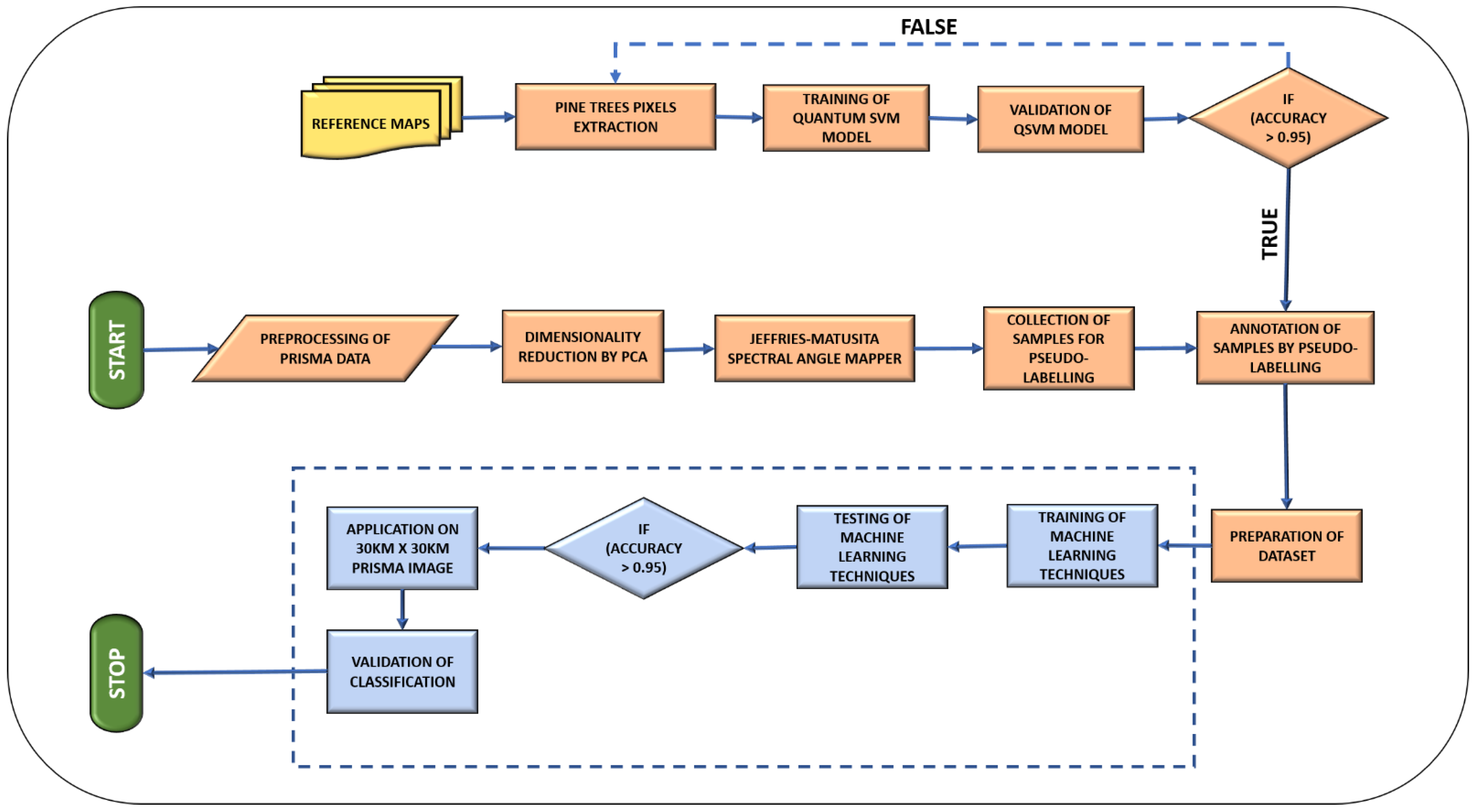
The flowchart shown in Figure 3 represents the process implemented for pseudo-labelling of the samples using QSVM. From the reference data, 20 pixels were selected that included 12 pine tree pixels; the remaining 8 pixels represented other vegetation and/or un-vegetation because a balanced dataset includes 60% positive and 40% negative samples [14]. In this work, a pixel represents the feature vector xn of dimension d = 16, and to each pixel, a label yn ∈ {0,1} was assigned, indicating the absence (0) or presence (1) of a pine tree. The dimensions of the feature vector were reduced from 196 to 16 using principal component (PC) analysis because it has been demonstrated by Riyaaz et al. [3] that it is possible to obtain the highest accuracy with 16 PCs of PRISMA data for vegetation classification. QSVM was trained using these 20 extracted samples.
Although the accuracy of QSVM is better than classical SVM for classification problems, it cannot be used for predicting all pixels of an image because of the limitation of the prediction speed. It was observed in the literature that QSVM takes around 7000 s to predict 50 samples whereas classical SVM takes only 1.2 s [3]. So, the use of QSVM is proposed for the preparation of a dataset of 600 samples. Using this accurate dataset, machine learning techniques that give a higher accuracy can be trained and implemented for prediction [1,3]. So, the JM-SAM method was applied to select 1000 similar samples from the image on which the trained QSVM was applied to predict 400 very similar samples as shown in Figure 3. The remaining 200 samples were selected randomly from the image, which included other vegetation types and non-vegetated pixels. Finally, a dataset of 600 pseudo-labelled samples was prepared in which 400 samples were positively annotated as ‘1’ and the remaining 200 samples were negatively annotated as ‘0’.

3.2. Inputs of ML Classifiers

Six ML techniques were considered in this study to identify the optimal technique for pine tree classification. Table 2 shows the input parameters considered for training the ML models of the six types referring to the literature. This study conducted Bayesian optimization to select the optimum parameters among the provided values of parameters. The same values of the parameters were used for the hybrid ML models as well.
Different kinds of optimization techniques give different values for the parameters. Zelin Huang et al. [17] proved that the parametric values differed between the genetic algorithm and grid search. For this demonstration, we chose Bayesian optimization in this study.

4. Results

4.1. Classification of Pine Trees

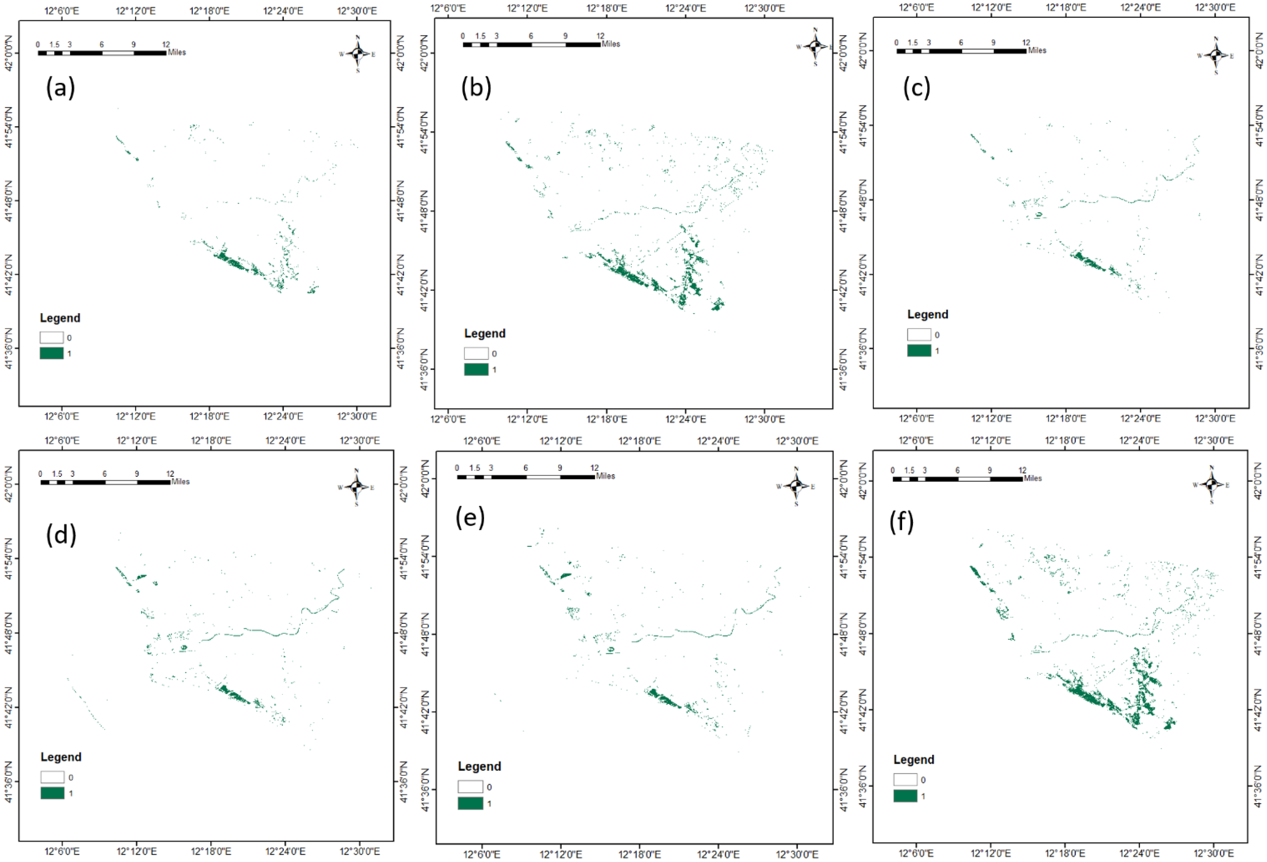
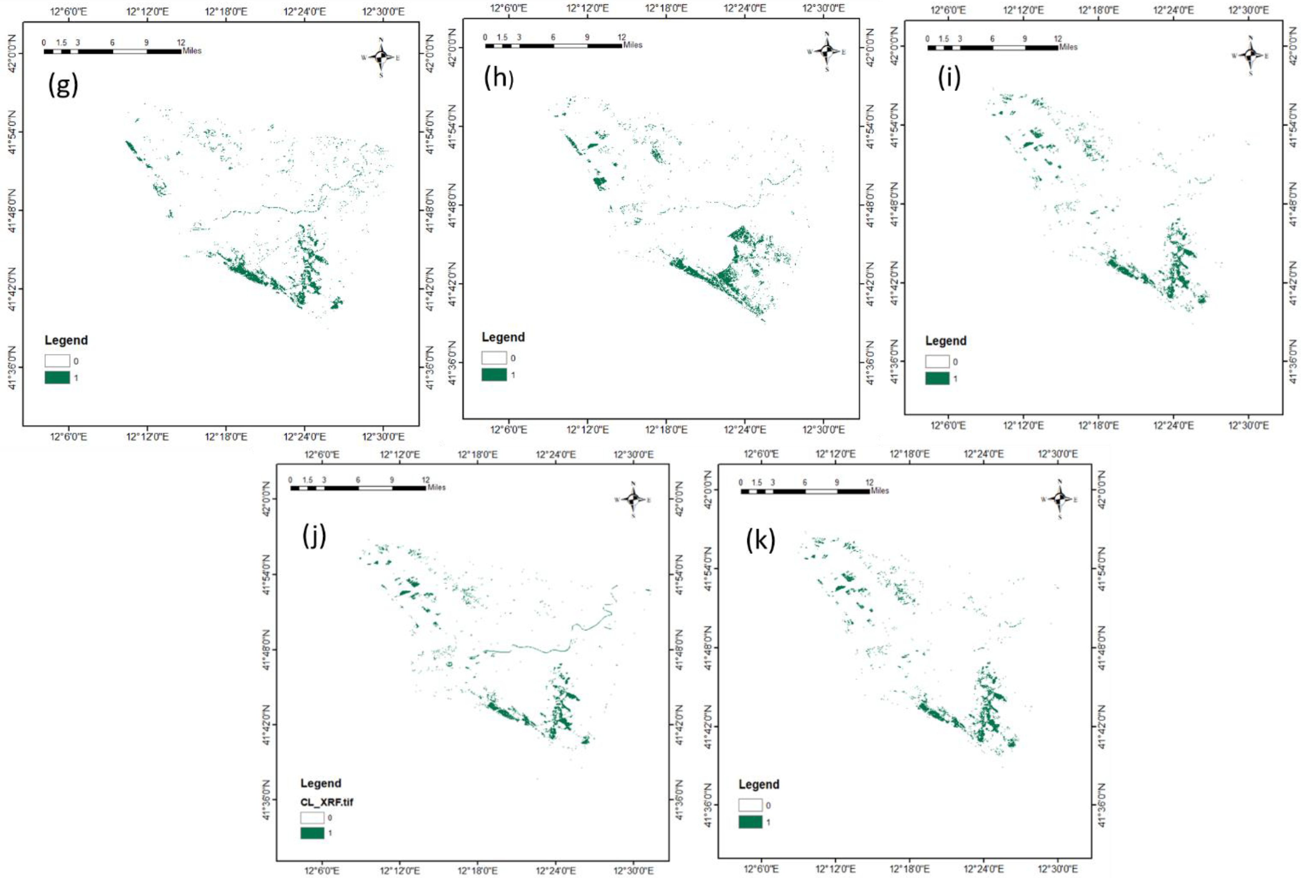
Figure 4 shows the pine tree classifications obtained using the quantum-based dataset and 11 different ML techniques. Table 2 shows the details of the classifiers implemented in the evaluation and the hyperparameters given as the input. The classifications were validated by comparing them with the reference data. In some of the classifications, vegetation near the river appears to be similar to the waves in the flow of the river.

4.2. Validation of the Pine Tree Classification

The pine tree classification was validated by randomly selecting 300 points in the classification and comparing each point with reference data, as shown in Table 3. As shown in Figure 4, different ML classifiers were applied to choose a suitable classifier for the classification of pine trees. Hybridised XGBoost, a tree-based algorithm that uses a gradient boosted framework, showed the best classification accuracy. XGBoost combined with a decision tree (DT) algorithm gave the best result in this study.

5. Discussions

Hyperspectral remote sensing has advanced significantly in the past decades. ML/DL techniques have become the most important tool in modern hyperspectral image analysis, especially for classification problems, because of their unprecedented predictive power. Additionally, the accuracy of machine learning-based classification depends entirely on the dataset. Therefore, to develop and evaluate machine learning-based classifications, annotated datasets have become most crucial. There is no single go-to dataset that serves the purpose of standardized benchmarking and pretraining due to the heterogeneity of remote sensing tasks and measurements. Thus, a dataset was prepared by pseudo-labelling samples using QSVM trained with 20 samples. In total, 20 samples were extracted, referring to the reference maps. Alternatively, a field survey can also easily be carried out to collect 12 data points for each vegetation, which could further increase the accuracy.
Another challenge of machine learning was also solved in this study, which is the selection of a suitable machine learning classifier for a specific task. The accuracy of ML algorithms depends on various factors such as the size of training data, dataset pattern, training parameters, etc., so selection based on accuracy is also tricky. In such cases, an optimal algorithm can be selected considering the number of classes, size and nature of training data, and predictor variables. In this work, considering these reasons, popular machine learning techniques were selected and trained using a quantum-based pseudo-labelled dataset to check the classification accuracy. XGBoost with the DCT hybrid ML technique trained with 600 pseudo-labelled samples gave a comparatively higher accuracy (86%) in classifying pine trees. This result can vary if other types of optimization models are used according to Huang, Z [17]. Another combination of XGBoost also performed slightly lower, with accuracies of 83%. From the classifications, it can be observed that some classifiers performed better in only one corner of the image, which may be at the top or bottom of the image, which may be due to mixed pixels. The bottom of the image has dense vegetation and the majority of the labelled data was selected from there whereas the top part of image has comparatively less vegetation with mixed pixels. So, spectral profiles extracted from mixed pixels lead to a decrease in the classification accuracy if classified using ML classifiers with broader thresholds.

6. Conclusions

This paper demonstrates the ability of QML to classify pine trees using the hybrid XGBoost + decision tree technique trained on a quantum-based pseudo-labelled dataset. Samples were pseudo-labelled for dataset preparation with QML using PRISMA hyperspectral imagery. It was proven that when there is no single go-to dataset, QML can be used for pseudo-labelling with ≤20 samples. Different ML classifiers were evaluated on a quantum-based dataset to find a suitable technique for the classification of pine trees. A hybrid technique (XGBoost + Decision Tree) gave promising results, with an accuracy of around 86%. The results show that QML pseudo-labelling and XGBoost hybrid classification can solve feature mapping and classification problems with accuracy within a modest processing time.

Author Contributions

Conceptualization, R.U.S., W.Z. and A.U.; methodology, R.U.S. and W.Z.; software, R.U.S. and A.U.; validation, R.U.S. and A.U.; formal analysis, R.U.S. and W.Z.; investigation, R.U.S. and W.Z.; resources, R.U.S.; data curation, R.U.S. and A.U.; writing—original draft preparation, R.U.S. and A.U.; writing—review and editing, R.U.S. and A.U.; visualization, R.U.S. and A.U.; supervision, R.U.S.; project administration, R.U.S. and A.U.; funding acquisition, W.Z. All authors have read and agreed to the published version of the manuscript.

Funding

This research is partially funded by Agtech Growth Fund (AGF) of Innovation Saskatchewan, Co. Labs, Canadian Agri-food Automation and Intelligence Network (CAAIN), and Mitacs.

Data Availability Statement

PRISMA imagery that support the findings of this study are accessed from Italian Space Agency’s (http://prisma.asi.it/) after the registration (ID: ITA_ScN1_0542_2$).

Acknowledgments

The authors would like to thank the IBM Quantum Challenge and EOSIAL Lab of Sapienza University of Rome, Italy for their support in carrying out this work.

Conflicts of Interest

The authors declare no conflict of interest.

References

  1. Gewali, U.B.; Monteiro, S.T.; Saber, E. Machine Learning Based Hyperspectral Image Analysis: A Survey. arXiv 2018, arXiv:1802.08701. [Google Scholar]
  2. Schmitt, M.; Ahmadi, S.A.; Hänsch, R. There is No Data Like More Data—Current Status of Machine Learning Datasets in Remote Sensing. arXiv 2021, arXiv:2105.11726. [Google Scholar]
  3. Shaik, R.U.; Periasamy, S. Accuracy and processing speed trade-offs in classical and quantum SVM classifier exploiting PRISMA hyperspectral imagery. Int. J. Remote Sens. 2022, 43, 6176–6194. [Google Scholar] [CrossRef]
  4. Huang, H.Y.; Broughton, M.; Mohseni, M.; Babbush, R.; Boixo, S.; Neven, H.; McClean, J.R. Power of Data in Quantum Machine Learning. Nat. Commun. 2021, 12, 2631. [Google Scholar] [CrossRef] [PubMed]
  5. Saini, S.; Khosla, P.; Kaur, M.; Singh, G. Quantum Driven Machine Learning. Int. J. Theor. Phys. 2020, 59, 4013–4024. [Google Scholar] [CrossRef]
  6. Arunachalam, S.; de Wolf, R. Guest Column: A Survey of Quantum Learning Theory 1. ACM SIGACT News 2017, 48, 41–67. [Google Scholar] [CrossRef] [Green Version]
  7. Biamonte, J.; Wittek, P.; Pancotti, N.; Rebentrost, P.; Wiebe, N.; Lloyd, S. Quantum Machine Learning. Nature 2017, 549, 195–202. [Google Scholar] [CrossRef] [PubMed] [Green Version]
  8. Ciliberto, C.; Herbster, M.; Ialongo, A.D.; Pontil, M.; Rocchetto, A.; Severini, S.; Wossnig, L. Quantum Machine Learning: A Classical Perspective. Proc. R. Soc. A Math. Phys. Eng. Sci. 2018, 474, 20170551. [Google Scholar] [CrossRef] [PubMed] [Green Version]
  9. Aaron, B.; Pelofske, E.; Hahn, G.; Djidjev, H.N. Using Machine Learning for Quantum Annealing Accuracy Prediction. Algorithms 2021, 14, 187. [Google Scholar] [CrossRef]
  10. Cavallaro, G.; Dennis, W.; Madita, W.; Kristel, M.; Morris, R. Approaching Remote Sensing Image Classification with Ensembles of Support Vector Machines on the D-Wave Quantum Annealer. In Proceedings of the IGARSS 2020—2020 IEEE International Geoscience and Remote Sensing Symposium, Waikoloa, HI, USA, 26 September–2 October 2020; pp. 1973–1976. [Google Scholar] [CrossRef]
  11. Otgonbaatar, S.; Datcu, M. A Quantum Annealer for Subset Feature Selection and the Classification of Hyperspectral Images. IEEE J. Sel. Top. Appl. Earth Obs. Remote Sens. 2021, 14, 7057–7065. [Google Scholar] [CrossRef]
  12. Liu, Y.; Arunachalam, S.; Temme, K. A Rigorous and Robust Quantum Speed-Up in Supervised Machine Learning. Nat. Phys. 2021, 17, 1013–1017. [Google Scholar] [CrossRef]
  13. Pepe, M.; Pompilio, L.; Gioli, B.; Busetto, L.; Boschetti, M. Detection and Classification of Non-Photosynthetic Vegetation from Prisma Hyperspectral Data in Croplands. Remote Sens. 2020, 12, 3903. [Google Scholar] [CrossRef]
  14. Shaik, R.U.; Giovanni, L.; Fusilli, L. New Approach of Sample Generation and Classification for Wildfire Fuel Mapping on Hyperspectral (Prisma) Image. In Proceedings of the 2021 IEEE International Geoscience and Remote Sensing Symposium IGARSS, Brussels, Belgium, 11–16 July 2021. [Google Scholar] [CrossRef]
  15. Amato, U.; Antoniadis, A.; Carfora, M.F.; Colandrea, P.; Cuomo, V.; Franzese, M.; Pignatti, S.; Serio, C. Statistical Classification for Assessing Prisma Hyperspectral Potential for Agricultural Land Use. IEEE J. Sel. Top. Appl. Earth Obs. Remote Sens. 2013, 6, 615–625. [Google Scholar] [CrossRef]
  16. Shaik, R.U.; Laneve, G.; Fusilli, L. An Automatic Procedure for Forest Fire Fuel Mapping Using Hyperspectral (PRISMA) Imagery: A Semi-Supervised Classification Approach. Remote Sens. 2022, 14, 1264. [Google Scholar] [CrossRef]
  17. Huang, Z.; Wu, W.; Liu, H.; Zhang, W.; Hu, J. Identifying Dynamic Changes in Water Surface Using Sentinel-1 Data Based on Genetic Algorithm and Machine Learning Techniques. Remote Sens. 2021, 13, 3745. [Google Scholar] [CrossRef]
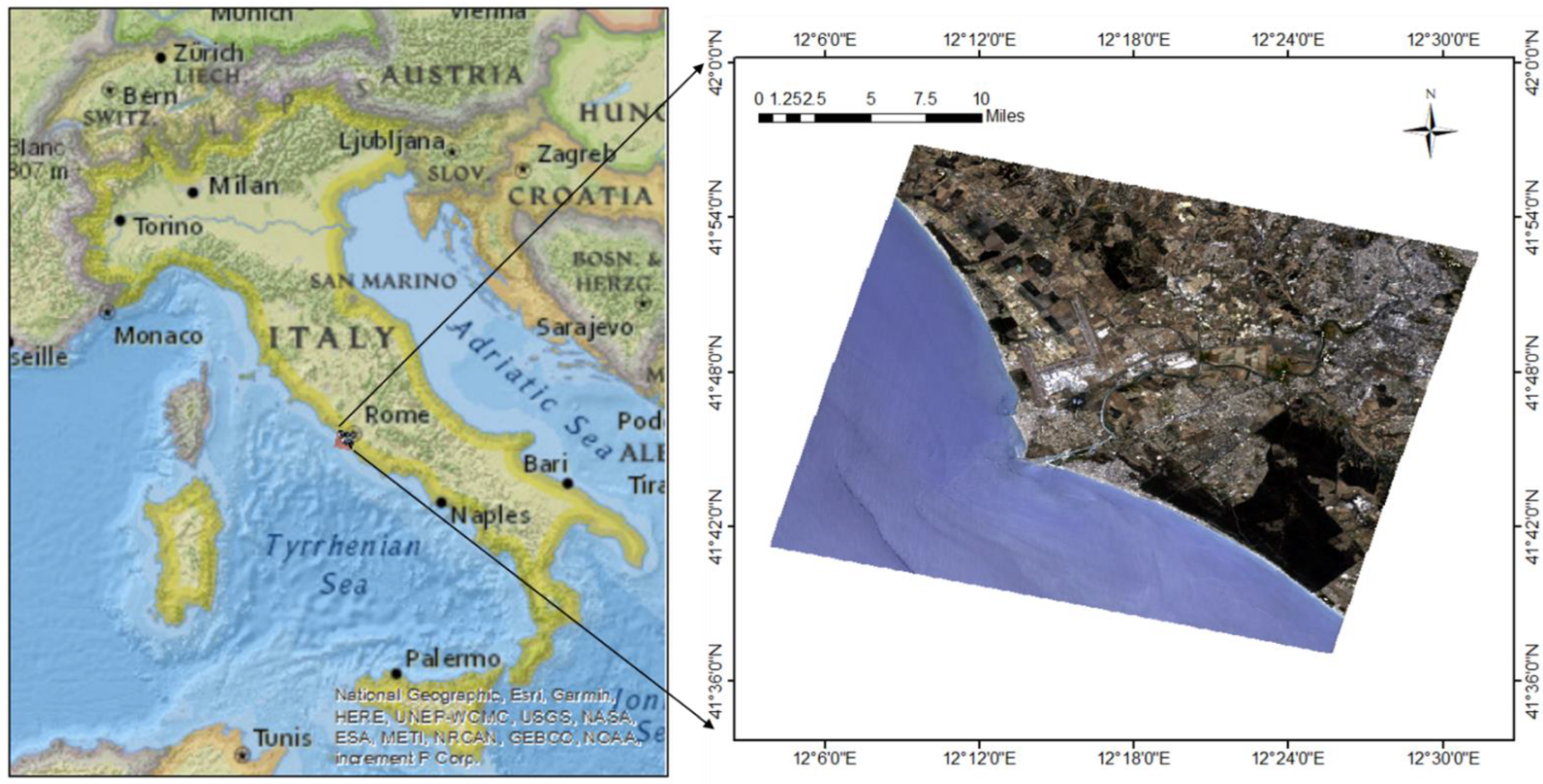
Figure 1. Region of interest (PRISMA image).
Remotesensing 14 05774 g001
Figure 2. Pine trees (genus Pinus)—reference data.
Remotesensing 14 05774 g002
Figure 3. Flowchart of the quantum-based pseudo-labelling of samples.
Remotesensing 14 05774 g003
Figure 4. Classification of pine trees using (a) SVM, (b) KNN, (c) Random Forest, (d) LGBM, (e) XGBoost, (f) SVC + Decision Tree, (g) Random Forest + SVC, (h) Random Forest + Decision Tree, (i) XGBoost + Decision Tree, (j) XGBoost + Random Forest, and (k) XGBoost + SVC.
Remotesensing 14 05774 g004aRemotesensing 14 05774 g004b
Table 1. Features of IBM backend.
Propertiesibmq_qasm_simulator
ProviderIbmq-q/open/main
status_msgActive
n_qubits32
backend_version0.1.547
basic_gatesU1, U2, U3, U, DELAY, P, R, RX, RY, RZ, ID, X, Y, Z, H, S, SDG, SX, T, TDG,
MULTIPLEXER, INITIALIZE, KRAUS, ROERROR, SWAP, CX, CY, CZ, CSX, CP, CU1, CU2, CU3, RXX, RYY, RZZ, RZX, CCX, CSWAP, MCX, MCY, MCZ, MCSX, MCP, MCU1, MCU2, MCU3, MCRX, MCRY, MCRZ, MCR, MCSWAP, UNITARY, DIAGONAL
max_circuits300
max_shots100,000
max_qubits per pulse gate3
max_channels per pulse gate9
Table 2. Details of the Machine Learning Classifiers.
S.NoMachine Learning TechniqueHyperparameters Range
1SVMC = (1,10,100), kernel = rbf and Gamma = (1 × 10⁻³ to 10)
2KNNn_neighbors = (5,7,9,11,13,15), weights = (‘uniform’, ’distance’), metric = (‘minkowski’, ’euclidean’, ’manhattan’)
3Random ForestBootstrap = (True, False), max_depth = (5,10,15,30), max_features = (2,3,5), min_sample_leaf = (2,5,10,100), min_sample_split = (2, 5, 10, 100), n_estimators = (100, 500)
4LGBMLearning_rate = (0.005, 0.01,0.01), n_estimator = (500), num_leaves = (6,30,50), boosting_type = (dart), max_depth = (1,3,5), max_bin = (225), reg_alpha = (1,1.2), reg_lambda = (1,1.2,1.4)
5XGBoostmin_child_weight = (1,3,5), subsample = (0.5,0.7)
6Decision Treemax_depth = (1,6,8,11), min_sample_split = (1,9,11), min_sample_leaf = (1,3,7,9)
Table 3. Validation Details of the Classification.
S.NoMachine Learning TechniqueValidation ResultTime Taken
(in Hours)
View on Classification Result
1SVMClassified Points = 243/300
Accuracy ≅ 80%
>2This model classified the pine trees and presented lower misclassification (less than 20%) of other vegetation.
2KNNClassified Points = 239/300
Accuracy ≅ 80%
>1This model classified the pine trees and presented higher misclassification (higher than 20%) of other vegetation (especially on upper part of the image).
3Random ForestClassified Points = 182/300
Accuracy ≅ 60%
>7Random forest did not classify all the pine trees; however, there were no misclassifications.
4LGBMClassified Points = 177/300
Accuracy ≅ 60%
>4LGBM did not classify all the pine trees; however, there were no noticeable misclassifications.
5XGBoostClassified Points = 182/300
Accuracy ≅ 60%
>1There was only a slight variation in XGBoost in comparison with LGBM, i.e., XGBoost classified a few more spots; however, the classification was insufficient.
6SVC + Decision TreeClassified Points = 241/300
Accuracy ≅ 80%
<1This model classified the pine trees very well, especially in the bottom part of the image.
7Random Forest + SVCClassified Points = 122/300
Accuracy ≅ 40%
<1This model misclassified other vegetation.
8Random Forest + Decision TreeClassified Points = 120/300
Accuracy ≅ 40%
<1This model misclassified other vegetation.
9XGBoost + Decision TreeClassified Points = 262/300
Accuracy ≅ 86%
<1This hybrid model classified the pine trees very well in the bottom region; however, it misclassified the top part.
10XGBoost + Random ForestClassified Points = 254/300
Accuracy ≅ 83%
<1This hybrid model classified the pine trees very well in the bottom region; however, it misclassified the top part.
11XGBoost + SVCClassified Points = 255/300
Accuracy ≅ 83%
<1This hybrid model classified the pine trees very well in the bottom region; however, it misclassified the top part.
Publisher’s Note: MDPI stays neutral with regard to jurisdictional claims in published maps and institutional affiliations.