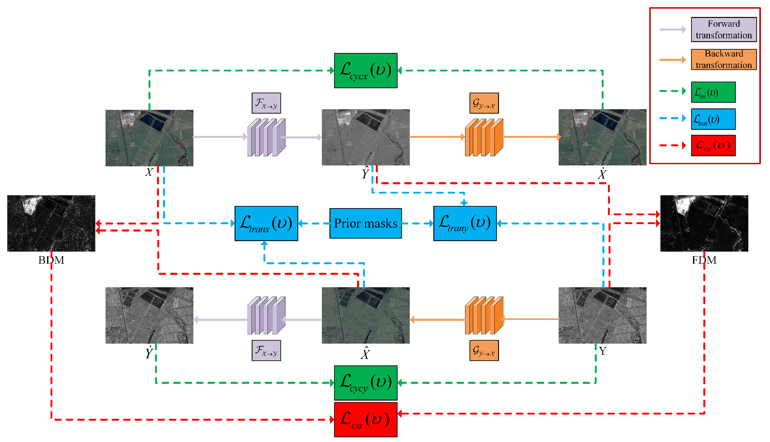
Figure 1.
Framework of the proposed CACD.
Figure 1.
Framework of the proposed CACD.
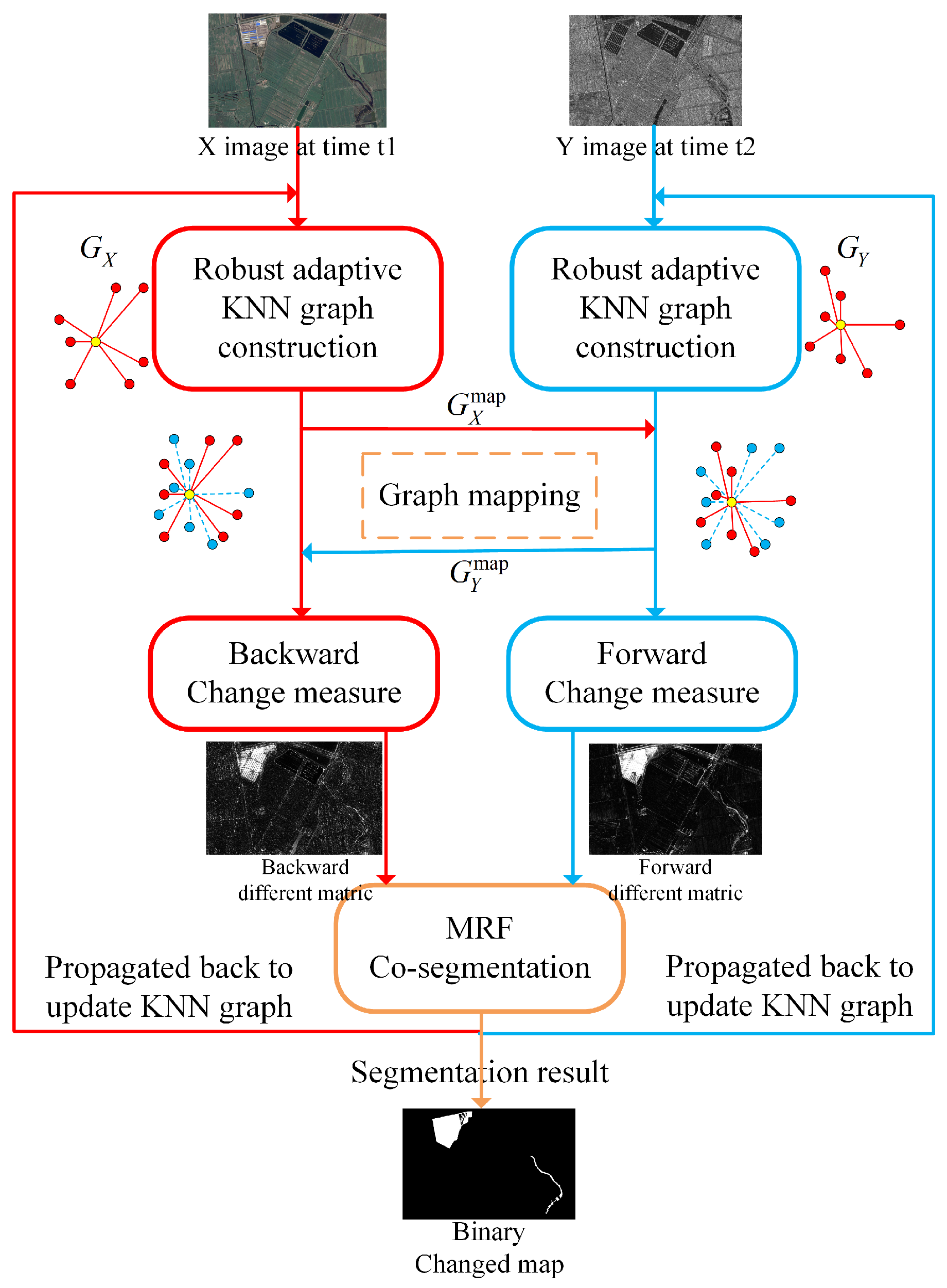
Figure 2.
Schematic diagram of IRG-McS.
Figure 2.
Schematic diagram of IRG-McS.
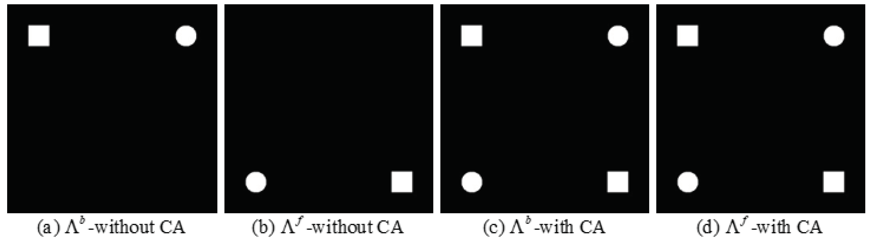
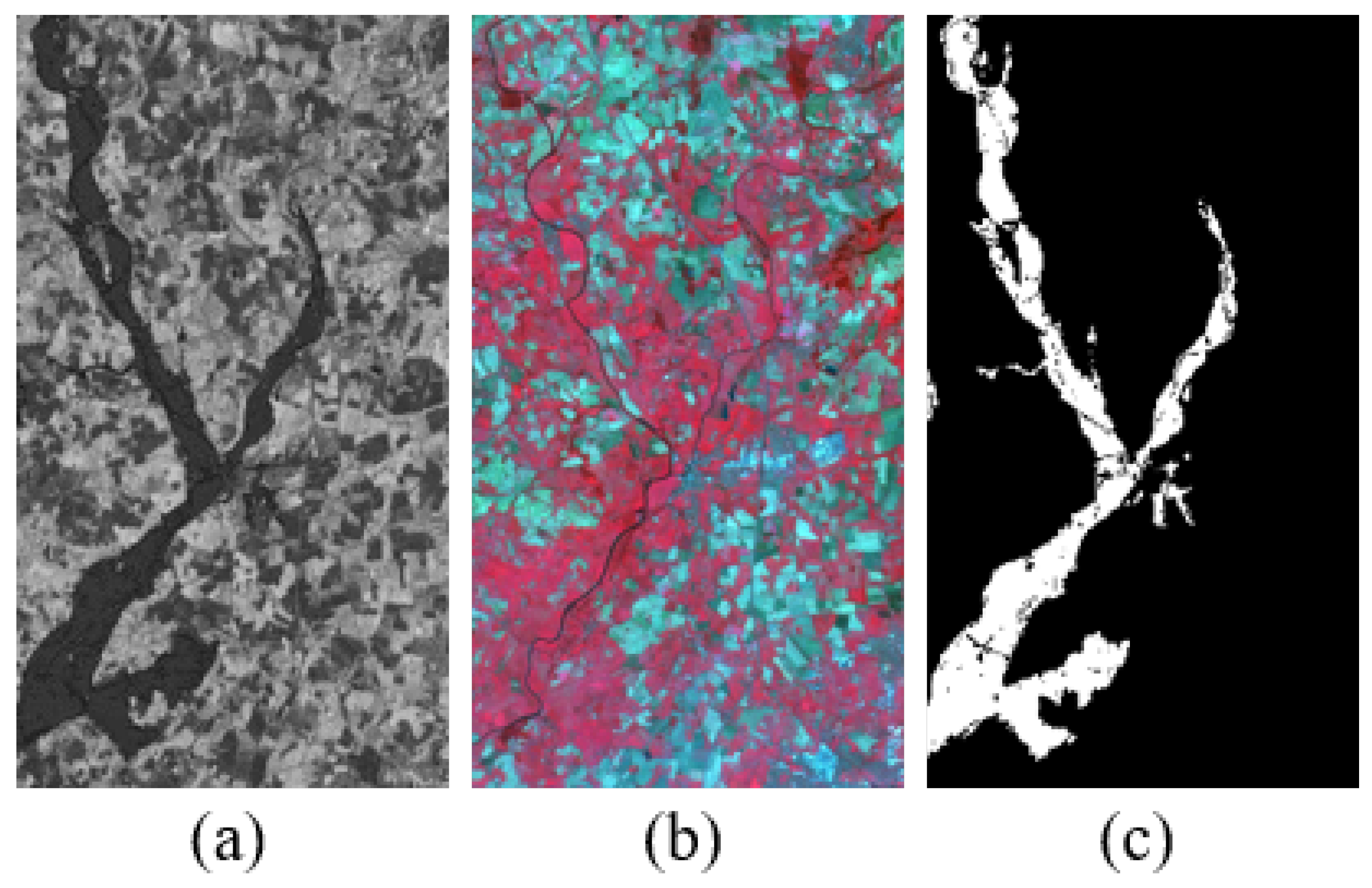
Figure 3.
Alignment of difference maps. (a) without the change alignment process. (b) without the change alignment process. (c) with the change alignment process. (d) with the change alignment process.
Figure 3.
Alignment of difference maps. (a) without the change alignment process. (b) without the change alignment process. (c) with the change alignment process. (d) with the change alignment process.
Figure 4.
California dataset. (a) Landsat-8 optical image. (b) Sentinel-1A SAR image. (c) Ground-truth.
Figure 4.
California dataset. (a) Landsat-8 optical image. (b) Sentinel-1A SAR image. (c) Ground-truth.
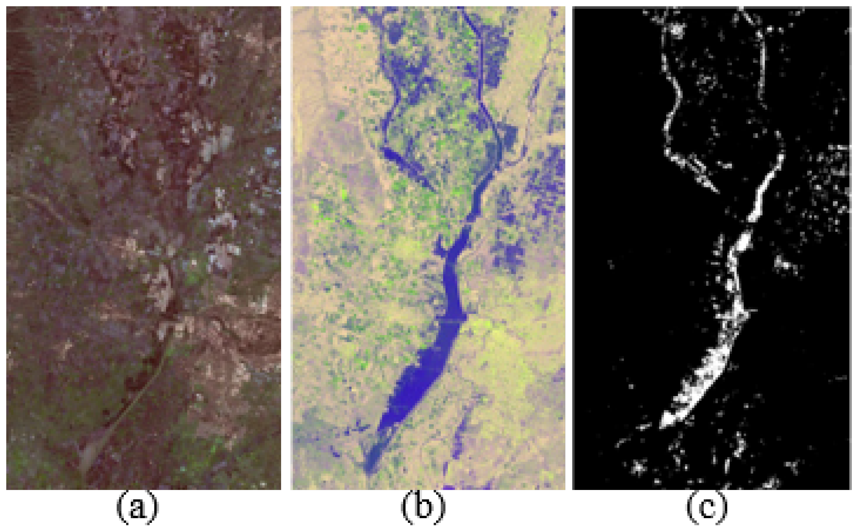
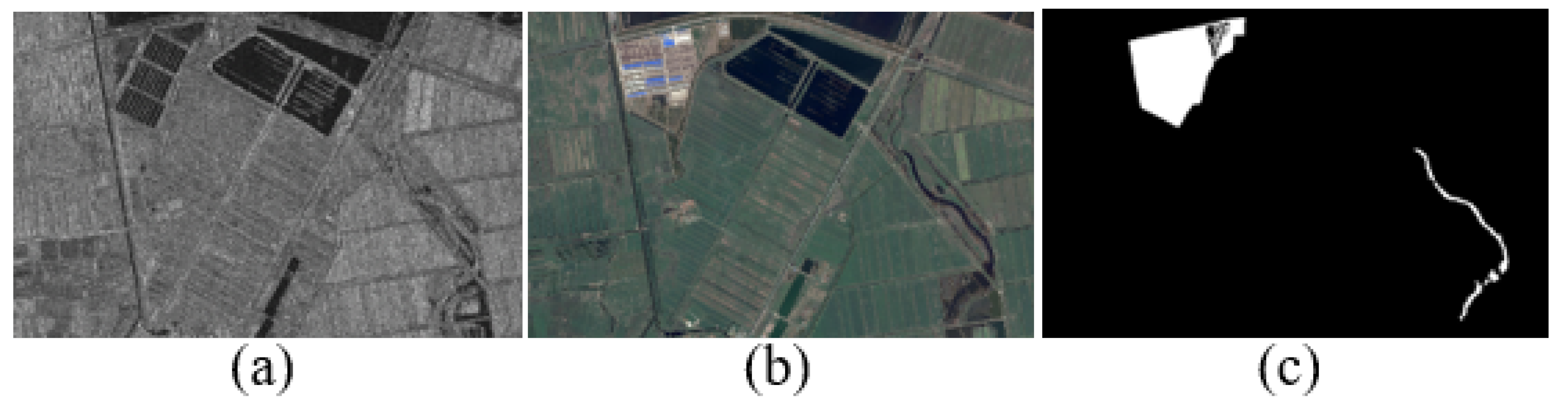
Figure 5.
Shuguang dataset. (a) Radarsat-2 SAR image. (b) Google Earth optical image. (c) Ground-truth.
Figure 5.
Shuguang dataset. (a) Radarsat-2 SAR image. (b) Google Earth optical image. (c) Ground-truth.
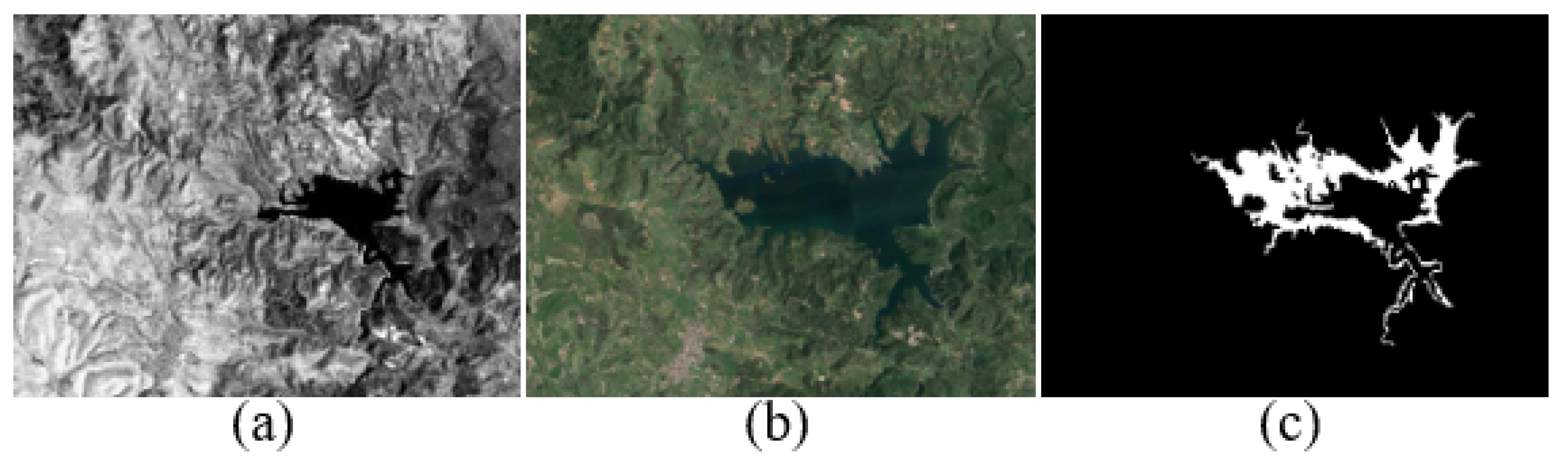
Figure 6.
Sardinia dataset. (a) Landsat-5 near-infrared image. (b) Google Earth optical image. (c) Ground-truth.
Figure 6.
Sardinia dataset. (a) Landsat-5 near-infrared image. (b) Google Earth optical image. (c) Ground-truth.
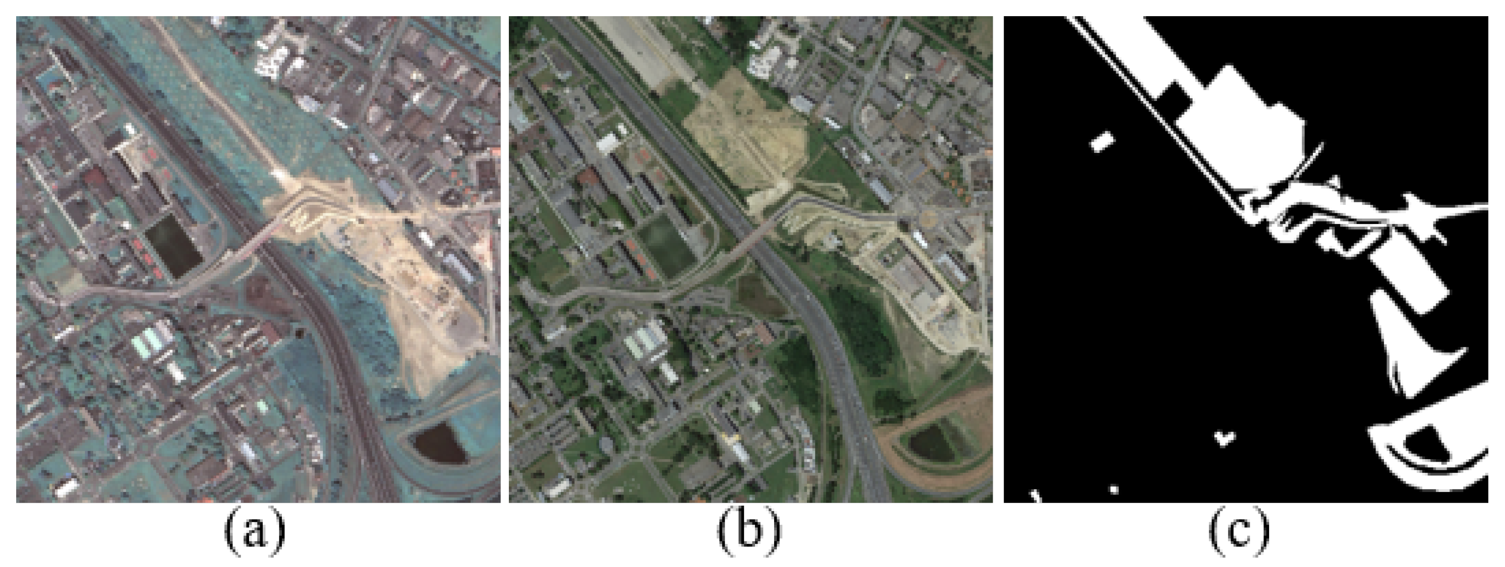
Figure 7.
Toulouse dataset. (a) Pleiades optical image. (b) WorldView2 optical image. (c) Ground-truth.
Figure 7.
Toulouse dataset. (a) Pleiades optical image. (b) WorldView2 optical image. (c) Ground-truth.
Figure 8.
Gloucester dataset (a) ERS image. (b) SPOT image. (c) Ground-truth.
Figure 8.
Gloucester dataset (a) ERS image. (b) SPOT image. (c) Ground-truth.
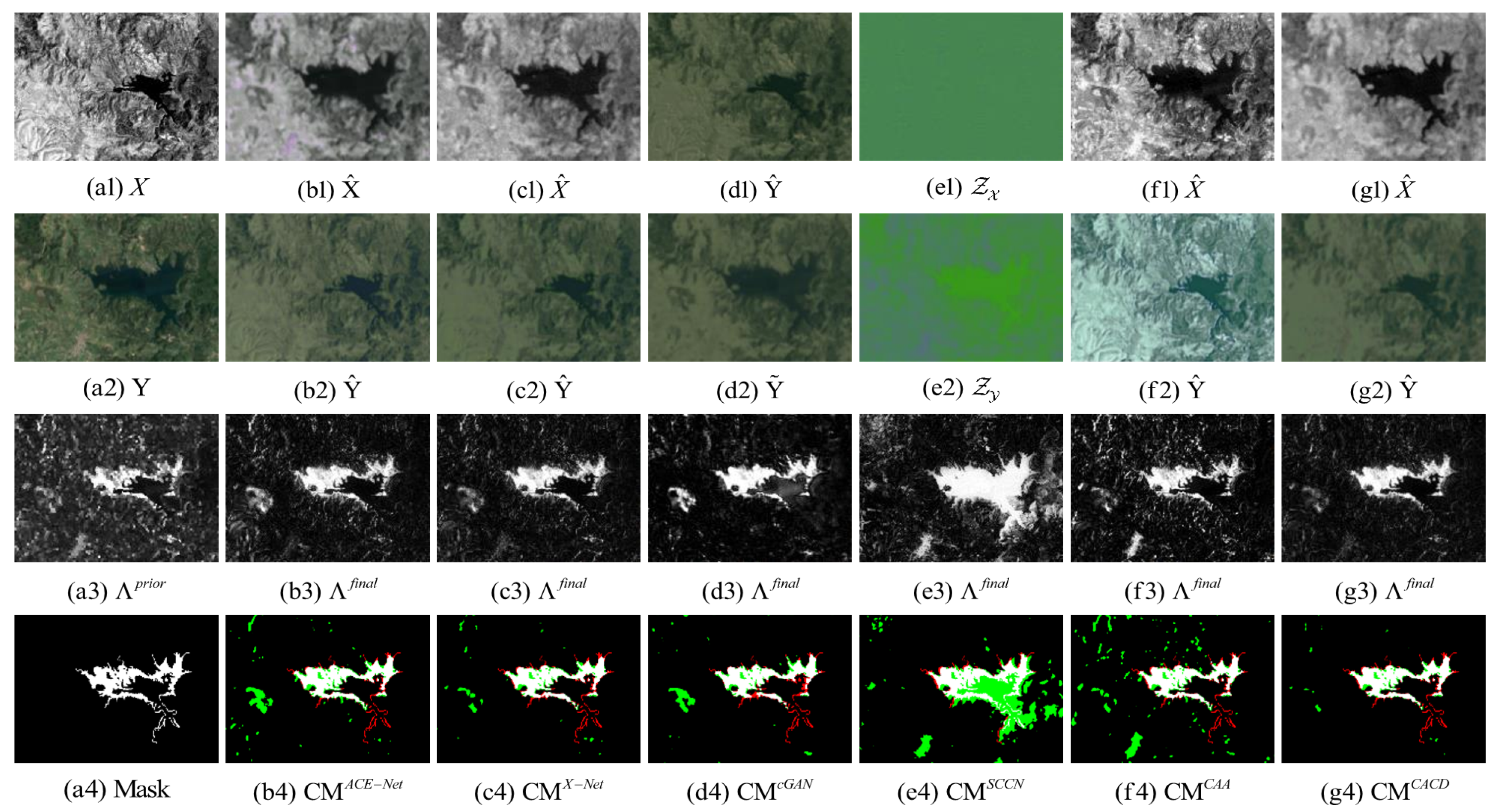
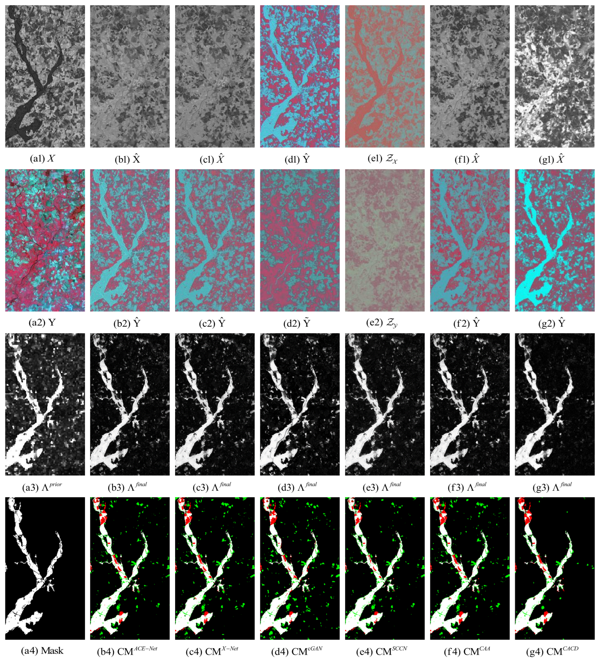
Figure 9.
California dataset. (a1) Input image X. (a2) Input image Y. (a3) Prior difference matrix generated by IRG-McS. (a4) Real mask. (b–g) represent the results of ACE-Net, X-Net, cGAN, SCCN, CAA and CACD (US) methods, respectively. (b1,c1,f1,g1) transformed image . (d1) transformed domain image . (e1) code image . (b2,c2,f2,g2) transformed image . (d2) approximate domain image . (e2) code image . (b3,c3,d3,e3,f3,g3) final difference map. (b4,c4,d4,e4,f4,g4) confusion map, where white: true positives (TP), black: true negatives (TN), green: false positives (FP), red: false negatives (FN).
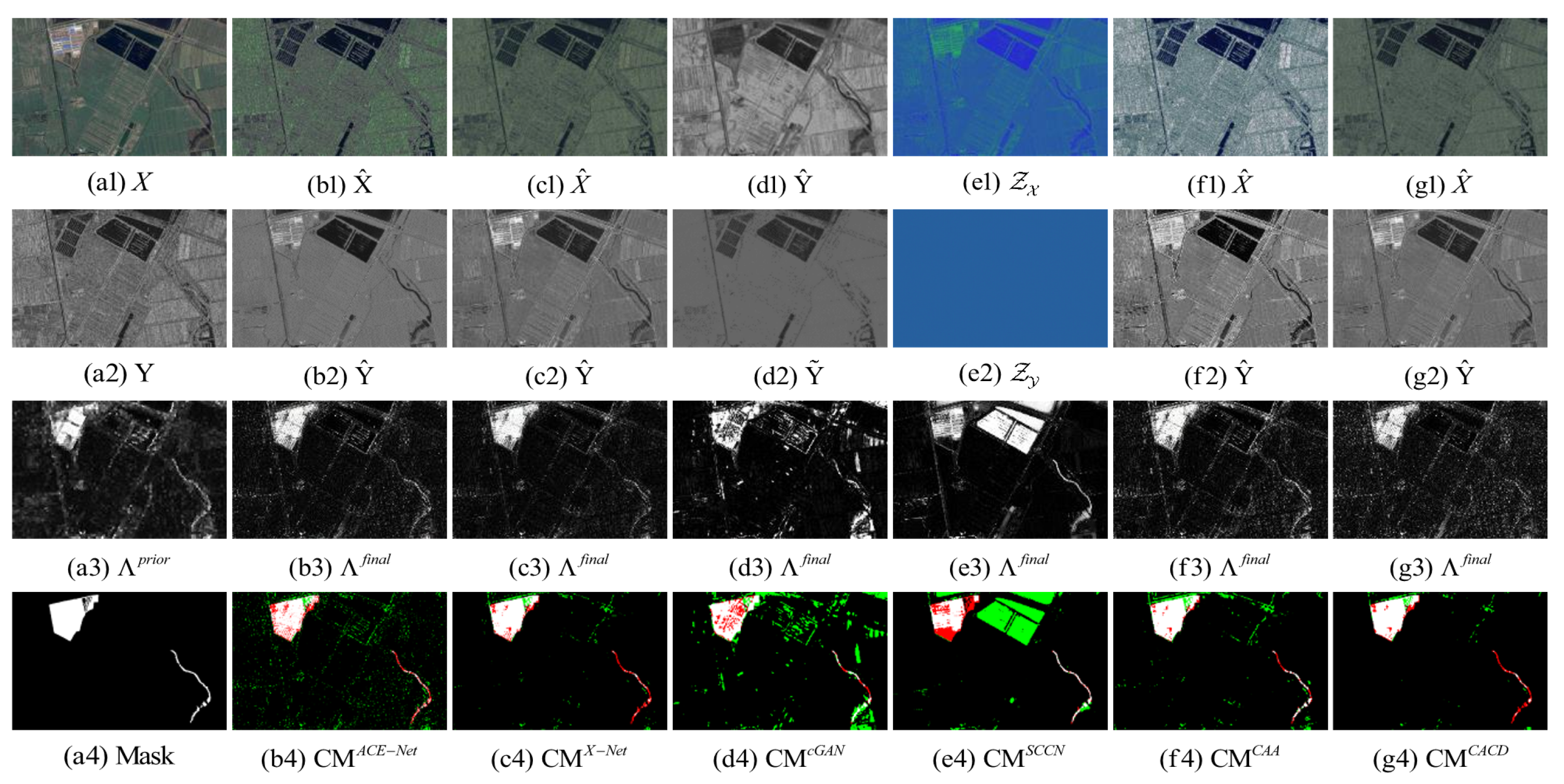
Figure 10.
Shuguang dataset. (a1) Input image X. (a2) Input image Y. (a3) Prior difference matrix generated by IRG-McS. (a4) Real mask. (b–g) represent the results of ACE-Net, X-Net, cGAN, SCCN, CAA and CACD (US) methods, respectively. (b1,c1,f1,g1) transformed image . (d1) transformed domain image . (e1) code image . (b2,c2,f2,g2) transformed image . (d2) approximate domain image . (e2) code image . (b3,c3,d3,e3,f3,g3) final difference map. (b4,c4,d4,e4,f4,g4) confusion map, where white: true positives (TP), black: true negatives (TN), green: false positives (FP), red: false negatives (FN).
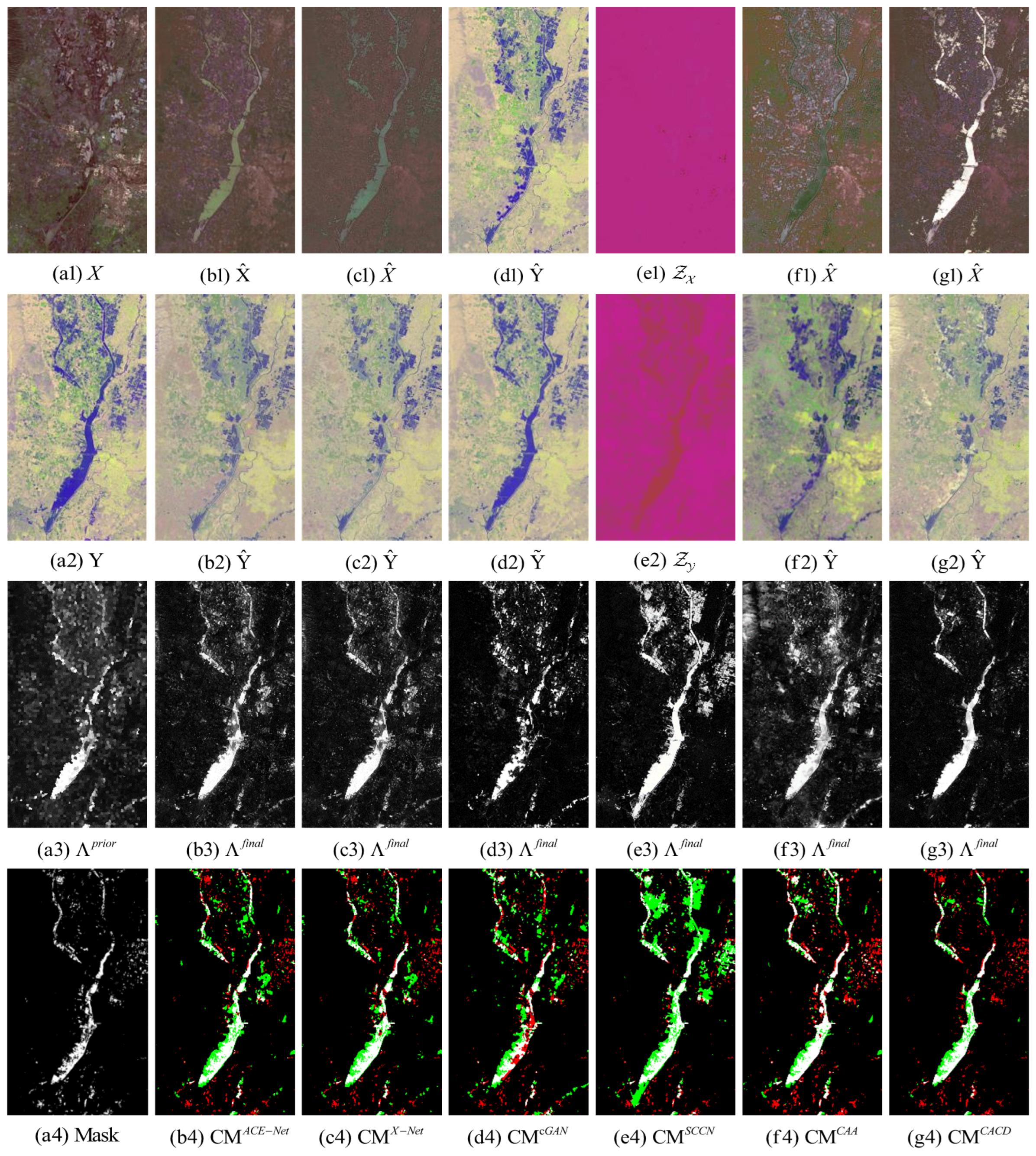
Figure 11.
Sardinia dataset. (a1) Input image X. (a2) Input image Y. (a3) Prior difference matrix generated by IRG-McS. (a4) Real mask. (b–g) represent the results of ACE-Net, X-Net, cGAN, SCCN, CAA and CACD (US) methods, respectively. (b1,c1,f1,g1) transformed image . (d1) transformed domain image . (e1) code image . (b2,c2,f2,g2) transformed image . (d2) approximate domain image . (e2) code image . (b3,c3,d3,e3,f3,g3) final difference map. (b4,c4,d4,e4,f4,g4) confusion map, where white: true positives (TP), black: true negatives (TN), green: false positives (FP), red: false negatives (FN).
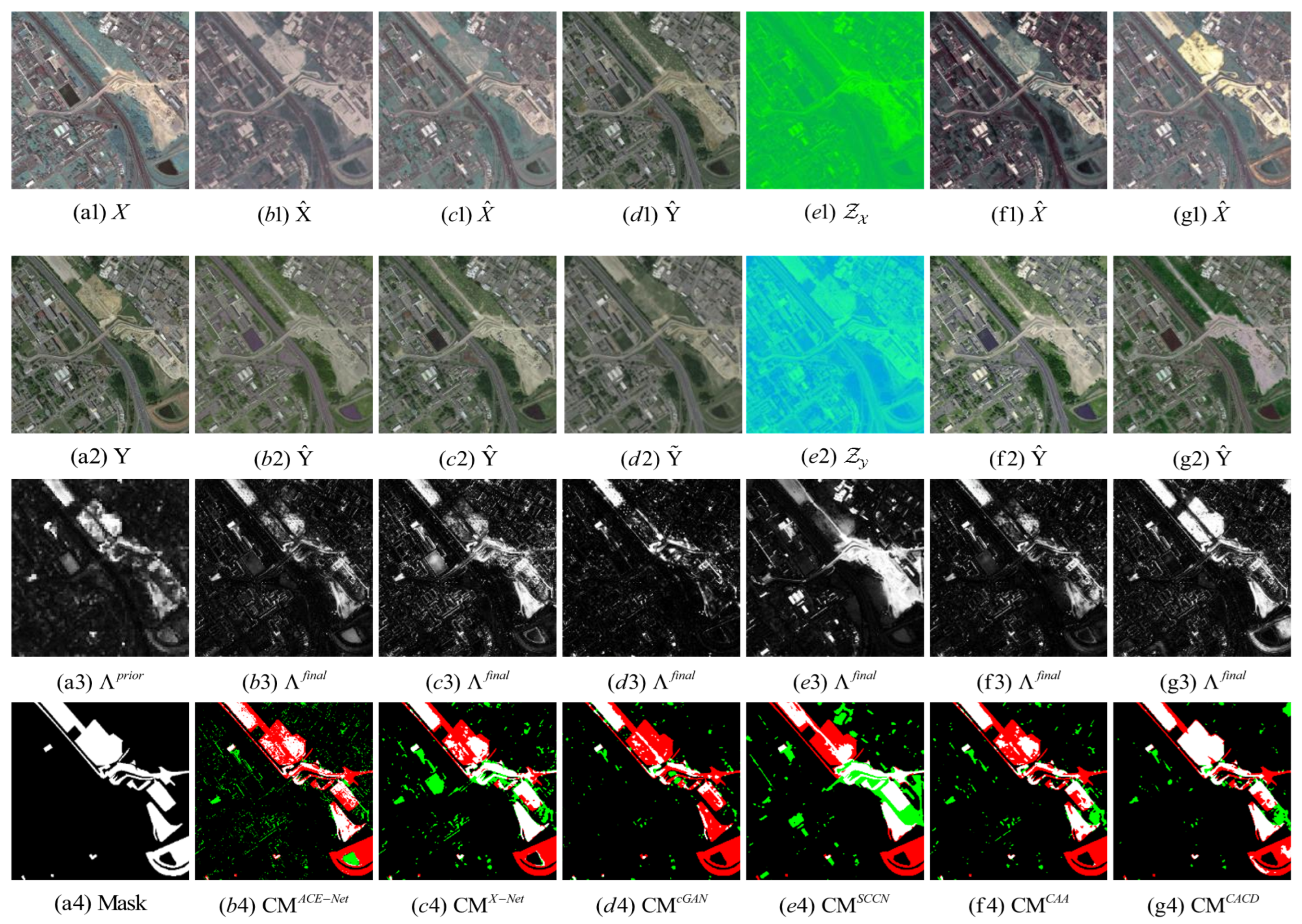
Figure 12.
Toulouse dataset. (a1) Input image X. (a2) Input image Y. (a3) Prior difference matrix generated by IRG-McS. (a4) Real mask. (b–g) represent the results of ACE-Net, X-Net, cGAN, SCCN, CAA and CACD (US) methods, respectively. (b1,c1,f1,g1) transformed image . (d1) transformed domain image . (e1) code image . (b2,c2,f2,g2) transformed image . (d2) approximate domain image . (e2) code image . (b3,c3,d3,e3,f3,g3) final difference map. (b4,c4,d4,e4,f4,g4) confusion map, where white: true positives (TP), black: true negatives (TN), green: false positives (FP), red: false negatives (FN).
Figure 13.
Gloucester dataset. (a1) Input image X. (a2) Input image Y. (a3) Prior difference matrix generated by IRG-McS. (a4) Real mask. (b–g) represent the results of ACE-Net, X-Net, cGAN, SCCN, CAA and CACD (US) methods, respectively. (b1,c1,f1,g1) transformed image . (d1) transformed domain image . (e1) code image . (b2,c2,f2,g2) transformed image . (d2) approximate domain image . (e2) code image . (b3,c3,d3,e3,f3,g3) final difference map. (b4,c4,d4,e4,f4,g4) confusion map, where white: true positives (TP), black: true negatives (TN), green: false positives (FP), red: false negatives (FN).
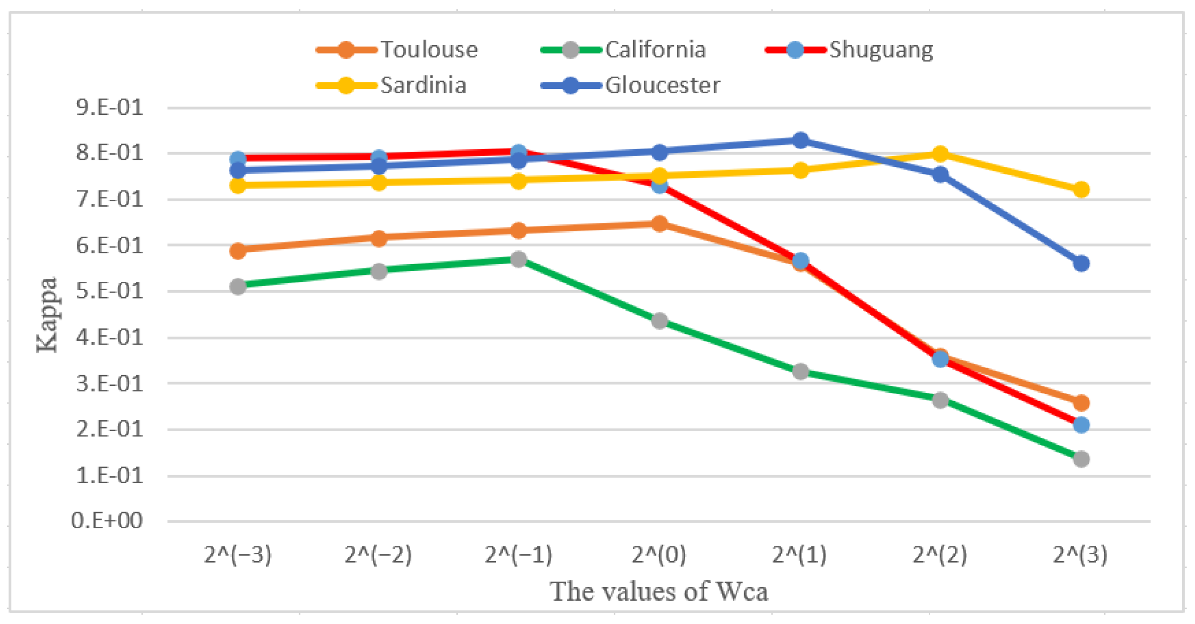
Figure 14.
Influences of parameter on the CACD performance.
Figure 14.
Influences of parameter on the CACD performance.
Table 1.
Quantitative evaluation on the California dataset.
Table 1.
Quantitative evaluation on the California dataset.
| | AUC | OA | Kc | |
|---|
| ACE-Net | 0.898 | 0.937 | 0.507 | 0.541 |
| X-Net | 0.901 | 0.941 | 0.513 | 0.545 |
| cGAN | 0.855 | 0.928 | 0.404 | 0.443 |
| SCCN | 0.928 | 0.910 | 0.466 | 0.510 |
| CAA | 0.891 | 0.940 | 0.576 | 0.609 |
| IRG-McS | 0.895 | 0.932 | 0.478 | 0.514 |
| CACD(US) | 0.912 | 0.953 | 0.566 | 0.590 |
Table 2.
Quantitative evaluation on the Shuguang dataset.
Table 2.
Quantitative evaluation on the Shuguang dataset.
| | AUC | OA | Kc | |
|---|
| ACE-Net | 0.964 | 0.981 | 0.788 | 0.798 |
| X-Net | 0.975 | 0.980 | 0.783 | 0.793 |
| cGAN | 0.912 | 0.934 | 0.482 | 0.514 |
| SCCN | 0.884 | 0.908 | 0.344 | 0.386 |
| CAA | 0.962 | 0.974 | 0.749 | 0.763 |
| IRG-McS | 0.980 | 0.964 | 0.668 | 0.686 |
| CACD(US) | 0.976 | 0.983 | 0.813 | 0.821 |
Table 3.
Quantitative evaluation on the Sardinia dataset.
Table 3.
Quantitative evaluation on the Sardinia dataset.
| | AUC | OA | Kc | |
|---|
| ACE-Net | 0.953 | 0.964 | 0.718 | 0.737 |
| X-Net | 0.943 | 0.972 | 0.764 | 0.778 |
| cGAN | 0.939 | 0.967 | 0.726 | 0.743 |
| SCCN | 0.920 | 0.899 | 0.478 | 0.523 |
| CAA | 0.933 | 0.951 | 0.642 | 0.667 |
| IRG-McS | 0.899 | 0.933 | 0.565 | 0.599 |
| CACD(US) | 0.954 | 0.977 | 0.800 | 0.812 |
Table 4.
Quantitative evaluation on the Toulouse dataset.
Table 4.
Quantitative evaluation on the Toulouse dataset.
| | AUC | OA | Kc | |
|---|
| ACE-Net | 0.802 | 0.882 | 0.477 | 0.540 |
| X-Net | 0.830 | 0.869 | 0.486 | 0.563 |
| cGAN | 0.752 | 0.864 | 0.320 | 0.379 |
| SCCN | 0.759 | 0.846 | 0.422 | 0.514 |
| CAA | 0.829 | 0.877 | 0.449 | 0.513 |
| IRG-McS | 0.893 | 0.903 | 0.575 | 0.628 |
| CACD(US) | 0.906 | 0.914 | 0.647 | 0.696 |
Table 5.
Quantitative evaluation on the Gloucester dataset.
Table 5.
Quantitative evaluation on the Gloucester dataset.
| | AUC | OA | Kc | |
|---|
| ACE-Net | 0.975 | 0.956 | 0.789 | 0.812 |
| X-Net | 0.972 | 0.954 | 0.767 | 0.791 |
| cGAN | 0.979 | 0.950 | 0.756 | 0.774 |
| SCCN | 0.988 | 0.960 | 0.810 | 0.834 |
| CAA | 0.976 | 0.948 | 0.774 | 0.805 |
| IRG-McS | 0.948 | 0.942 | 0.714 | 0.749 |
| CACD(US) | 0.987 | 0.963 | 0.834 | 0.854 |
Table 6.
Ablation study on the Toulouse dataset.
Table 6.
Ablation study on the Toulouse dataset.
| | AUC | OA | Kc | |
|---|
| (1) | 0.906 | 0.914 | 0.646 | 0.696 |
| (2) | 0.864 | 0.889 | 0.567 | 0.630 |
| (3) | 0.899 | 0.903 | 0.621 | 0.676 |
| (4) | 0.839 | 0.871 | 0.499 | 0.575 |
Table 7.
Ablation study on the California dataset.
Table 7.
Ablation study on the California dataset.
| | AUC | OA | Kc | |
|---|
| (1) | 0.912 | 0.953 | 0.566 | 0.590 |
| (2) | 0.909 | 0.945 | 0.536 | 0.565 |
| (3) | 0.902 | 0.954 | 0.556 | 0.581 |
| (4) | 0.903 | 0.935 | 0.496 | 0.531 |
Table 8.
Ablation study on the Shuguang dataset.
Table 8.
Ablation study on the Shuguang dataset.
| | AUC | OA | Kc | |
|---|
| (1) | 0.976 | 0.983 | 0.813 | 0.821 |
| (2) | 0.976 | 0.981 | 0.789 | 0.799 |
| (3) | 0.956 | 0.984 | 0.812 | 0.821 |
| (4) | 0.971 | 0.979 | 0.767 | 0.778 |
Table 9.
Ablation study on the Sardinia dataset.
Table 9.
Ablation study on the Sardinia dataset.
| | AUC | OA | Kc | |
|---|
| (1) | 0.954 | 0.977 | 0.800 | 0.812 |
| (2) | 0.955 | 0.975 | 0.785 | 0.799 |
| (3) | 0.952 | 0.976 | 0.794 | 0.807 |
| (4) | 0.947 | 0.974 | 0.775 | 0.788 |
Table 10.
Time efficiency analysis on the five datasets.
Table 10.
Time efficiency analysis on the five datasets.
| | California | Shuguang | Sardinia | Toulouse | Gloucester |
|---|
| ACE-Net | 1536.37 s | 1735.79 s | 895.47 s | 1105.06 s | 1829.34 s |
| X-Net | 1114.42 s | 1306.92 s | 484.34 s | 684.46 s | 1347.13 s |
| cGAN | 963.52 s | 990.79 s | 446.15 s | 933.75 s | 1029.38 s |
| SCCN | 325.18 s | 386.43 s | 140.32 s | 229.90 s | 416.52 s |
| CAA | 1684.52 s | 1812.07 s | 1053.89 s | 1287.36 s | 1897.90 s |
| IRG-McS | 9.37 s | 9.52 s | 8.03 s | 8.56 s | 9.64 s |
| CACD(US) | 398.73 s | 406.64 s | 389.53 s | 393.03 s | 413.42 s |


