1. Introduction
To observe Earth quickly and timely, new-generation meteorological satellites usually run at geostationary orbits with low spatial resolutions. Typical geostationary satellites include the U.S. GOES-16, Japan’s Himawari-8, Europe’s MTG-I, and China’s Fengyun-4. The low spatial resolution ensures that they can observe clouds and rainfall in a timely manner given the limited physical size and signal-to-noise ratio of the sensors. However, with the continuous demand for improved accuracy in weather forecasting, a higher spatial resolution is desired to discern weather differences across geographic locations. From a software perspective, the need can be partially addressed by super-resolution.
Super-resolution of meteorological images is a reconstruction problem that has been studied for decades. During the imaging process of weather satellites, sunlight reflected from the Earth’s surface undergoes atmospheric turbulence, lens blurring and satellite motion before reaching the sensor. Geometric corrections in the post-processing process also lose detail. The super-resolution we wish to perform is not only resolution improvement but also detail recovery, but it is a classical illness-posed inverse problem because a low-resolution image can be obtained by downsampling from an infinite number of different high-resolution images. To improve this problem, constrained models, optimization methods, and prior knowledge can be targeted [
1].
There is a long-term need for standardized super-resolution datasets to benchmark various methods under the same conditions. There have been many super-resolution datasets for natural images. Early datasets include Set5, Set14, B100, and Urban100. The development of deep learning calls for far larger data volume, so new datasets are proposed, such as the well-known DIV2K and Flickr2K [
2], and Flickr30K [
3]. However, for remotely sensed applications, such datasets are still absent, especially when deep learning is used for remote sensing [
4,
5,
6,
7].
Remote sensing datasets are usually designed for segmentation, classification, change detection, or object detection. For example, with images from the Google Earth platform, [
8] designed the LoveDA dataset for segmentation, [
9] designed the S
UC dataset for urban village classification, and [
10] designed the FAIR1M dataset along with the Gaofen-1 images for object detection. The HSI-CD dataset [
11] from the EO-1 Hyperion images can be used for hyperspectral change detection.
Unfortunately, there are no available datasets from meteorological satellites for super-resolution benchmark. Very few datasets on weather images are related to cloud segmentation. Ref. [
12] designed the 38-Cloud dataset consisting of 8400 patches of 18 scenes for training and 9201 patches of 20 scenes for testing. Patches are extracted from the Landsat 8 Collection 1 Level-1 scenes with four visible bands. Later, they extended the dataset to the 95-Cloud dataset [
13] consisting of 34,701 patches of 75 scenes for training. The test sets in 95-Cloud and 38-Cloud are the same. The patch size is
for 38-Cloud and 95-Cloud datasets. Similar work was done by [
14], who proposed a new Landsat-8 dataset (WHU cloud dataset) for simultaneous cloud detection and removal. The dataset consists of six cloudy and cloud-free image pairs in different areas. However, these cloud images are time independent and do not show time continuity, and the image size is too small to learn sufficiently for large-scale neural networks.
To fill the gap of super-resolution meteorological datasets, this paper presents two new super-resolution datasets from the visible bands of the Fengyun-4A (or FY4A) [
15] satellite designed for cloud detection. One dataset is a single-channel 8-bit quantized dataset, and the other is a 3-channel 16-bit quantized dataset. Low-resolution images in our datasets are accompanied with corresponding 4-times high-resolution images. The size of the high-resolution images is 10,992 × 4368 which is far larger than the size in commonly used datasets. The total scale of our dataset is comparable to that of DIV2K. However, due to the low resolution, there is less structural information in images, which makes the performance of super-resolution algorithms for natural images necessary of being re-evaluated. The single-channel 8-bit quantized dataset can be used to quickly test the effectiveness of the existing super-resolution algorithms, as it requires no modification to existing code. The 3-channel 16-bit quantized dataset is more realistic to real scenarios of remote sensing application pursuing accurate digital numbers for further quantitative analysis.
The proposed datasets differ from existing datasets for two reasons. On the one hand, since the meteorological satellites focus on adverse air conditions, such as cloud, fog, rain, haze, and so on, their need for super-resolution are reasonably different from commonly used datasets. On the other hand, meteorological satellite images have very high temporal resolutions which creates an image sequence giving the chance for the study of spatiotemporal fusion [
16] or spatiotemporal-spectral fusion [
17]. The framework of generative adversarial network (GAN) can be used for this topic which is investigated in [
18]. Consequently, the super-resolution methods for the proposed datasets can be of more variety to make full use of the repeated scanning as time-series images provide far richer information than images in single-patch super resolution.
In order to evaluate the performance when the datasets are used for super-resolution, state-of-the-art algorithms are used. Our experiments try to touch the performance boundaries of the super-resolution algorithms from the perspective of quantitative remote sensing. That is, we try to uncover how much the best super-resolution algorithm can affect the reconstruction error. The conclusion can be used to assess the practical possibilities of super-resolution algorithms on the proposed dataset.
The following contributions are made in our work.
- (1)
We present two medium-resolution remote sensing datasets that are the first meteorological datasets and are almost temporally continuous.
- (2)
We validate the performance bounds of existing single-image super-resolution algorithms on the datasets to provide the baseline for performance improvement.
The remainder of the paper is structured as follows.
Section 2 introduces the FY4ASR dataset.
Section 3 introduces the experimental schemes, including the state-of-the-art super-resolution algorithms, training strategies, 16-bit preprocessing, and metrics for image quality assessment.
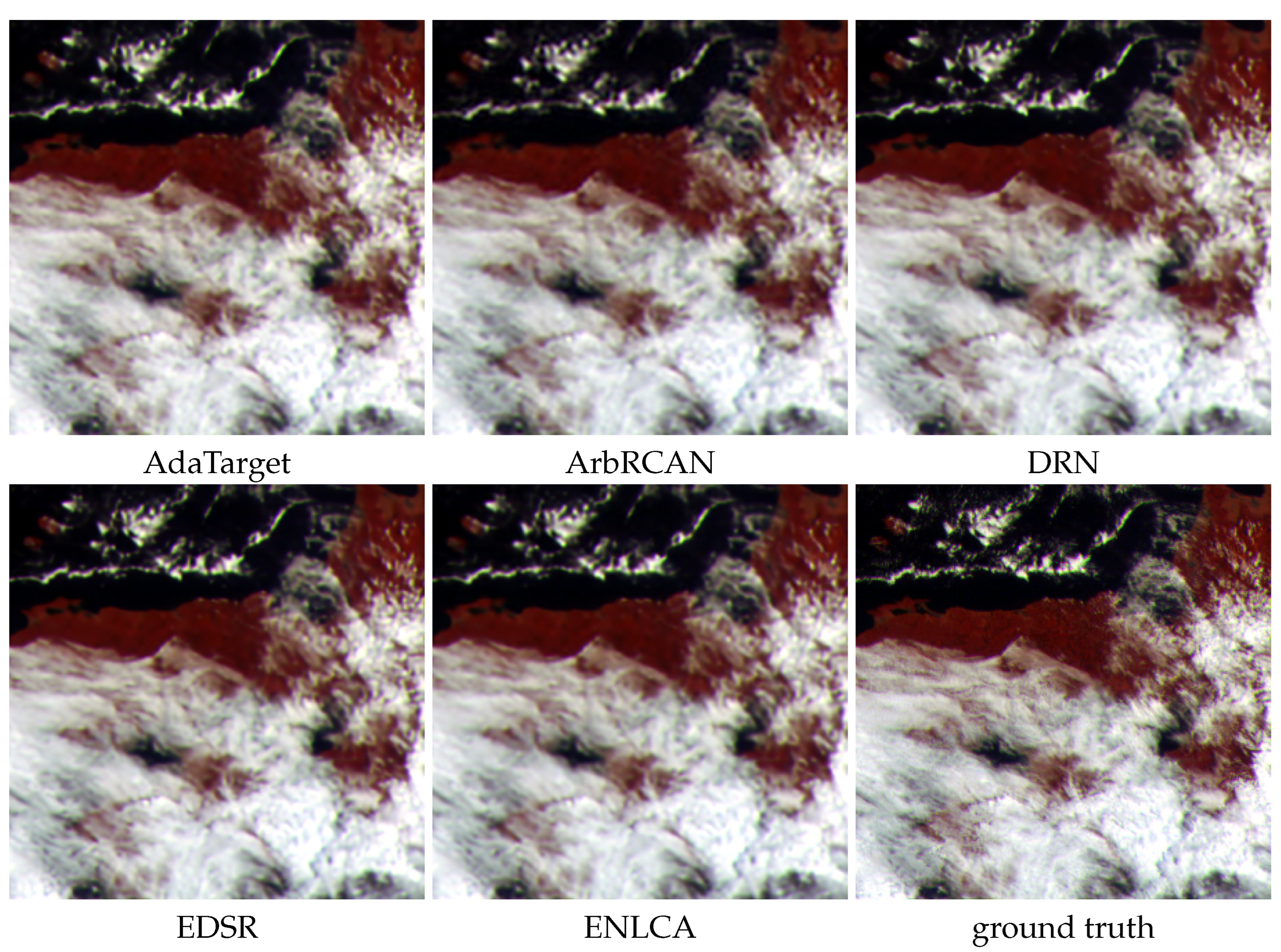
Section 4 presents the experimental results which are evaluated visually and digitally.
Section 5 gives the conclusion.
2. Proposed FY4ASRgray and FY4ASRcolor Datasets
We propose the FY4ASRgray and FY4ASRcolor datasets for benchmarking both time-based and example-based image super-resolution algorithms. These two datasets are captured by the FengYun-4A (or FY4A) satellite launched by China in 2016 and equipped with sensors, such as Advanced Geostationary Radiation Imager (AGRI) [
19], Geostationary Interferometric Infrared Sounder (GIIRS), and Lightning Mapping Imager (LMI).
AGRI is the main payload which has a complex double-scanning mirror mechanism enabling both precise and flexible imaging modes. The flexible mode allows for quick scanning at high minute rates with the loss of spatial resolution, while the precise scans slowly for higher spatial resolutions. AGRI in FY4A has 14 channels with the 0.5–1 km resolutions for visual light (450–490 nm, 550–750 nm) or near infrared (750–900 nm) bands, and 2–4 km for infrared (2.1–2.35 µm) bands. AGRI spends 15 min for full-disc scanning to present a global cloud image. On-board black body is available for calibration of infrared bands at very short time intervals.
The proposed two super-resolution datasets differ in bit length and channel number. Images in FY4ASRgray are 8-bit quantized with single channel, while images in FY4ASRcolor are 16-bit quantized with three channels. All images in FY4ASRgray and FY4ASRcolor are paired, where the ground resolutions are 1 km for high-resolution images and 4 km for low-resolution images. Ref. [
20] have tried the 8-bit FY4A data for super-resolution, but the 16-bit reconstruction is far challenging.
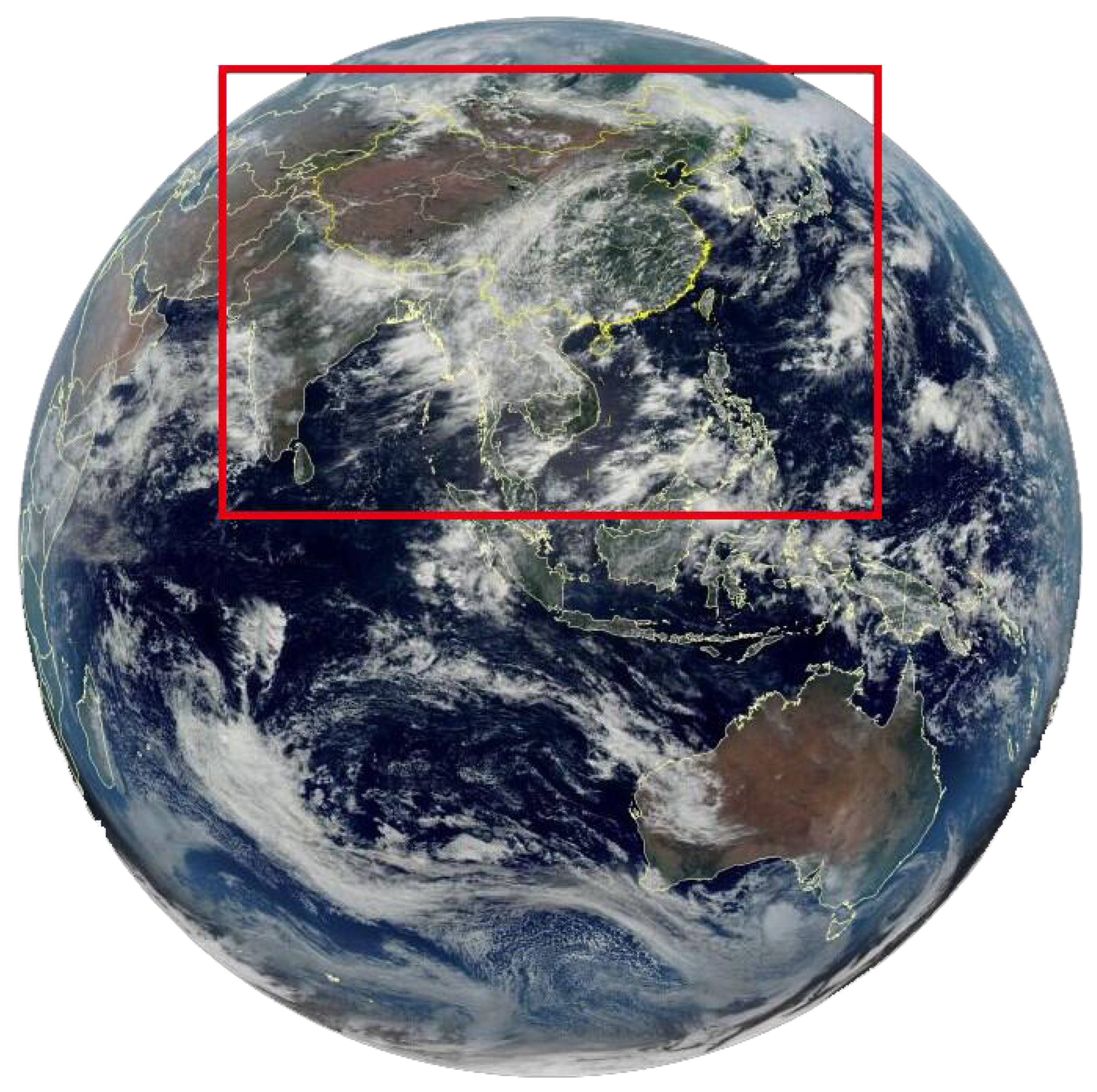
The images in FY4ASRgray and FY4ASRcolor datasets are all captured by AGRI full disc scanning covering China (region of China, REGC, see
Figure 1) with the 5-min time interval for regional scanning. The images were originally quantized using 16 bits, and the valid range of the data is 0 to 4095. However, many super-resolution algorithms are designed for natural images where 16 bits cannot be fed in. At this point, FY4ASRgray can be used to test the effectiveness of these algorithms. However, the quantization accuracy of FY4ASRgray is insufficient and the spectral information is lost due to the single channel. In contrast, FY4ASRcolor serves to reconstruct the rich information more accurately using the multi-channel information for subsequent segmentation and classification applications, which is in line with the purpose of remote sensing.
FY4ASRgray uses the second band of ARGI spanning the spectral range 550–750 nm for fog and cloud detection. The images were captured between 26 and 27 August 2021, and preprocessed at level 1 including radiometric and geometric corrections. The Level-1 images were then enhanced and quantized to 8-bit integer types ranging from 0 to 255 and stored using lossy JPEG format.
FY4ASRcolor datasets uses the first three bands of AGRI, namely blue (450–490 nm), red-green (550–750 nm), and visible NIR (750–900 nm). The images were captured on 16 September 2021. All the bands are in 16-bit data format after radiometric and geometric correction for Level-1 preprocessing, and stored using lossless TIFF format.
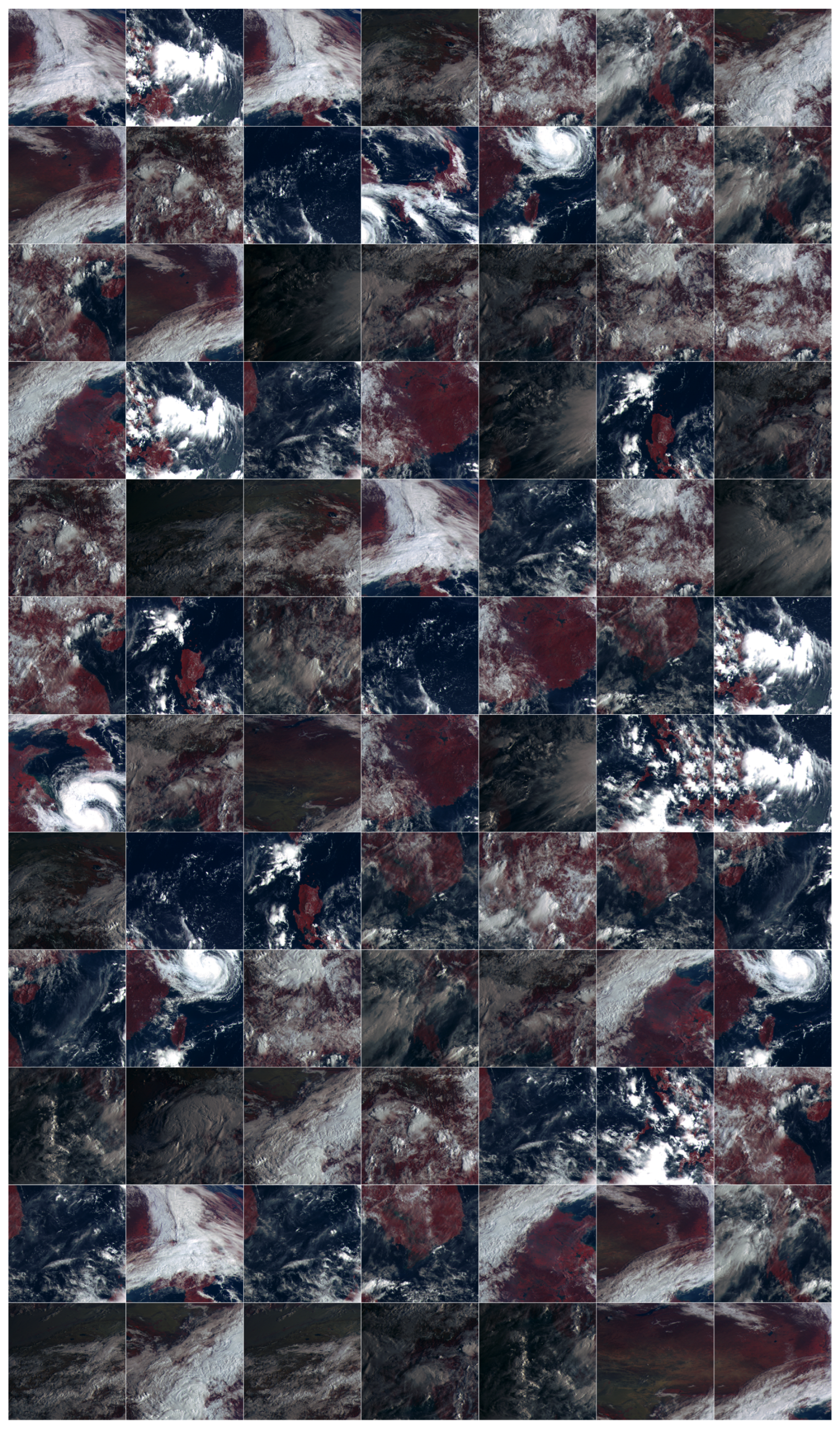
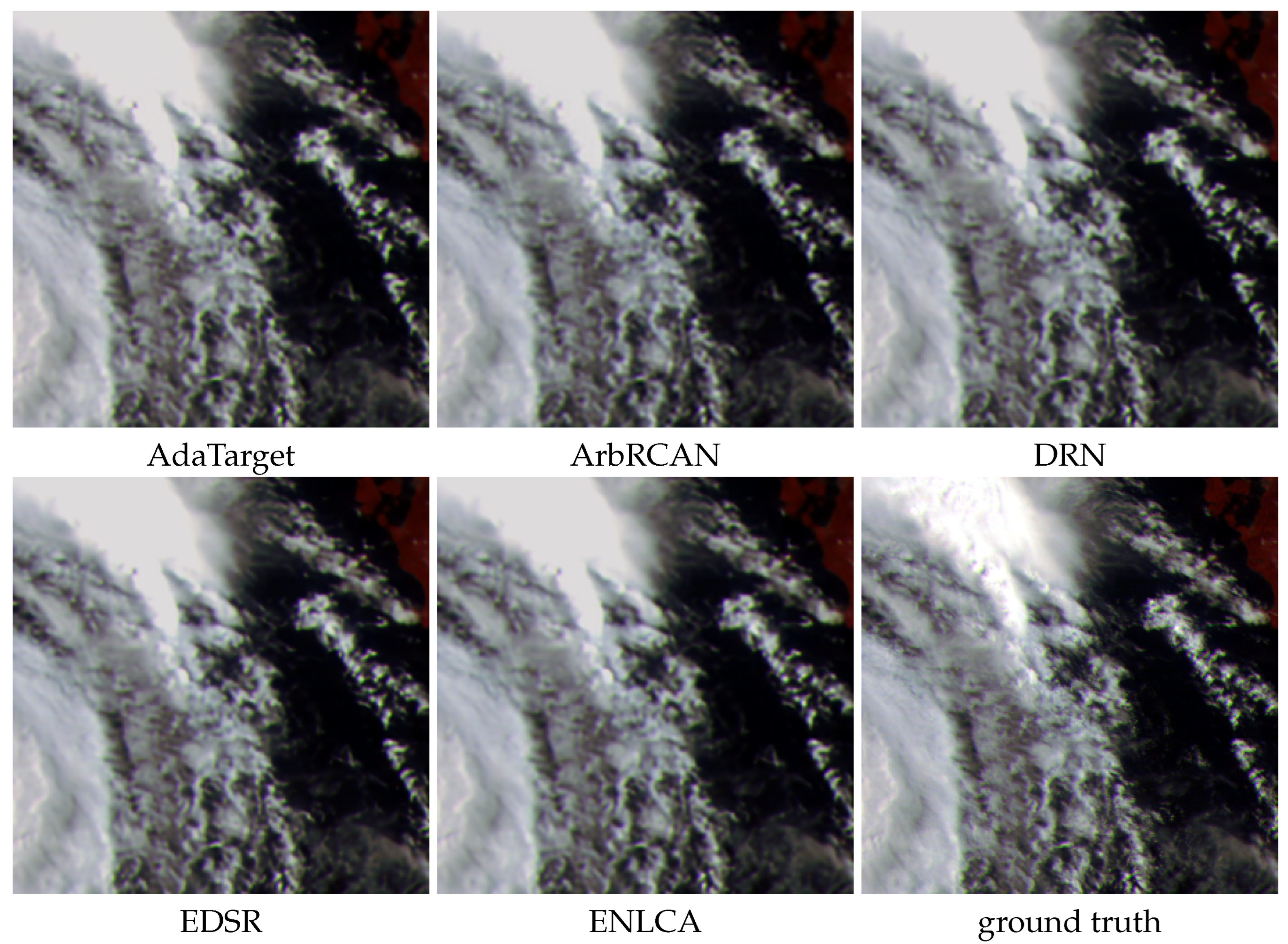
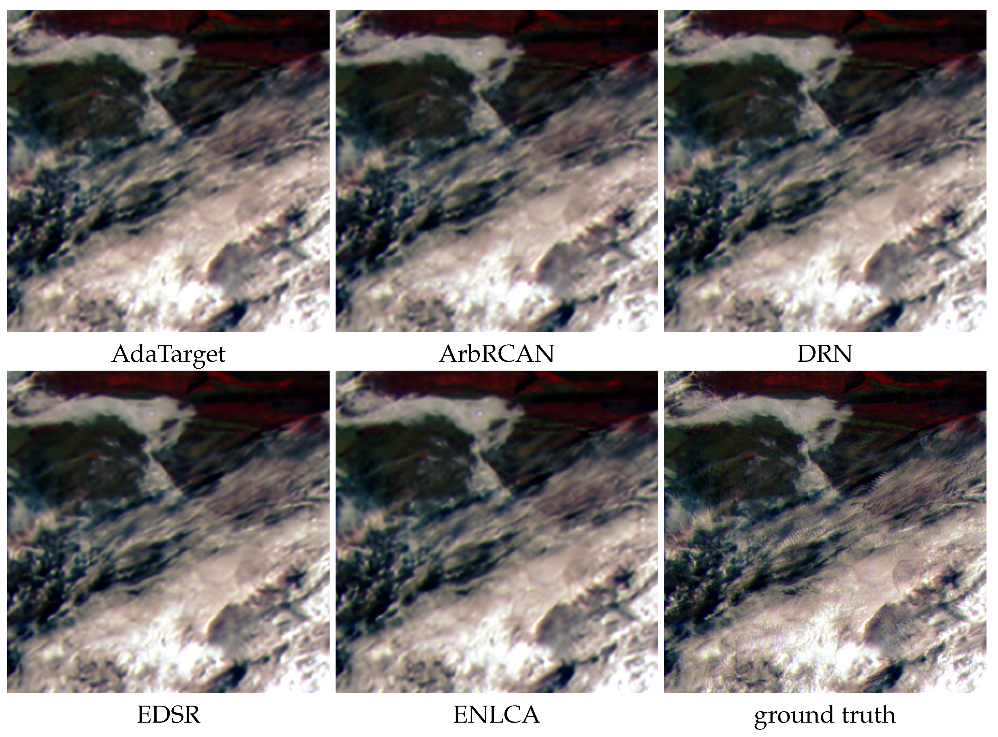
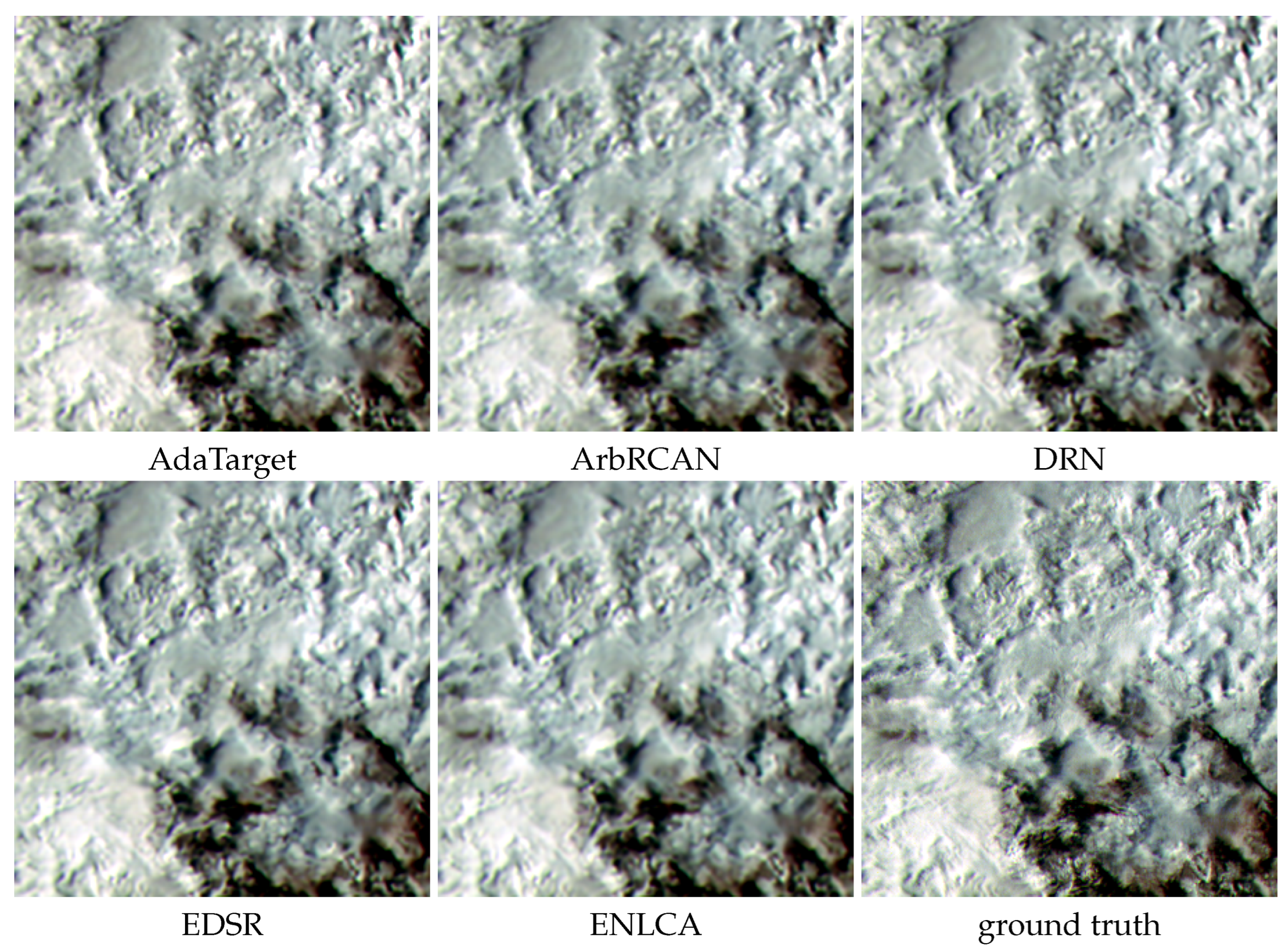
Figure 2 presents some patches from the FY4ASRcolor datasets that are non-linearly enhanced. Since the actual quantization is 12 bits, each digital number ranges from 0 to 4095, but the vast majority of values are between 50 and 2100. Considering that many existing algorithms have codes that limit the input within the range 0 to 255, the input and output of existing algorithms needs to be modified to accommodate 16 bits when using their codes.
In terms of data scale, our FY4ASRgray and FY4ASRcolor datasets are comparable to widely used large-scale natural image datasets. FY4ASRgray contains 130 pairs of images, while FY4ASRcolor contains 165 pairs of images. The size of the high resolution image is 10,992 × 4368 and the size of the low resolution image is 2748 × 1092. After eliminating the invalid area, the darkest 1.5% of pixels, and the brightest 1.5% of pixels in FY4ASRcolor, the average percentage of valid pixels is 64.85% and the number of valid pixels is 5.14 billions. In contrast, the number of pixels in the DIV2K dataset is 6.69 billions.
It has to be noted that the low-resolution images in FY4ASRgray and FY4ASRcolor are not downsampled from the high-resolution images, but are acquired by separately mounted sensors of the same type. In addition to the spatial difference, there are minor differences between these two types of images, which we call the sensor difference. Possible causes of the sensor difference include various spectral response curves, solar altitude angles, preprocessing methods, and so on, which makes the difference stochastic and scene dependent [
16]. After downsampling the high-resolution images and comparing them with the low-resolution images, the average absolute errors are 1.619 for FY4ASRgray and 29.63 for FY4ASRcolor. To obtain the optimal super-resolution performance, it is necessary for algorithms to model the sensor difference.
3. Experimental Scheme
The FY4A dataset file can be downloaded from the URL
github.com/isstncu/fy4a, accessed on 25 October 2022, which takes up 39.1 GB of disk size. To test the usability of the new datasets, state-of-the-art super-resolution algorithms are gathered for contest. The technique of shift learning is used to shorten the training time and approach to the optimal parameters. The reconstruction results will be evaluated with objective metrics. The super-resolution algorithms, evaluation metrics, and the additional 16-bit processing are described in this section.
3.1. Methods for Validation
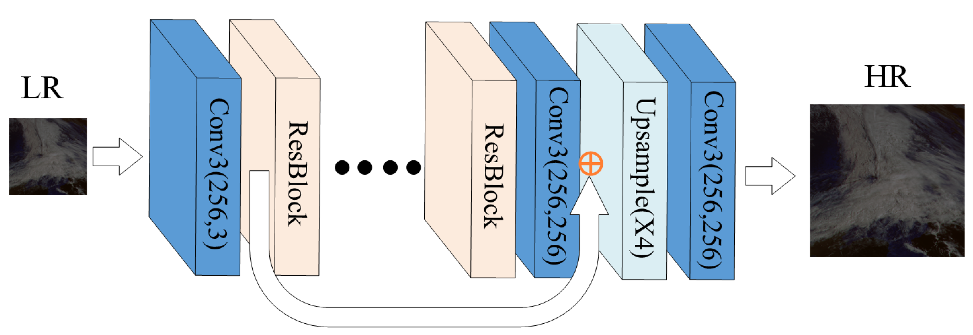
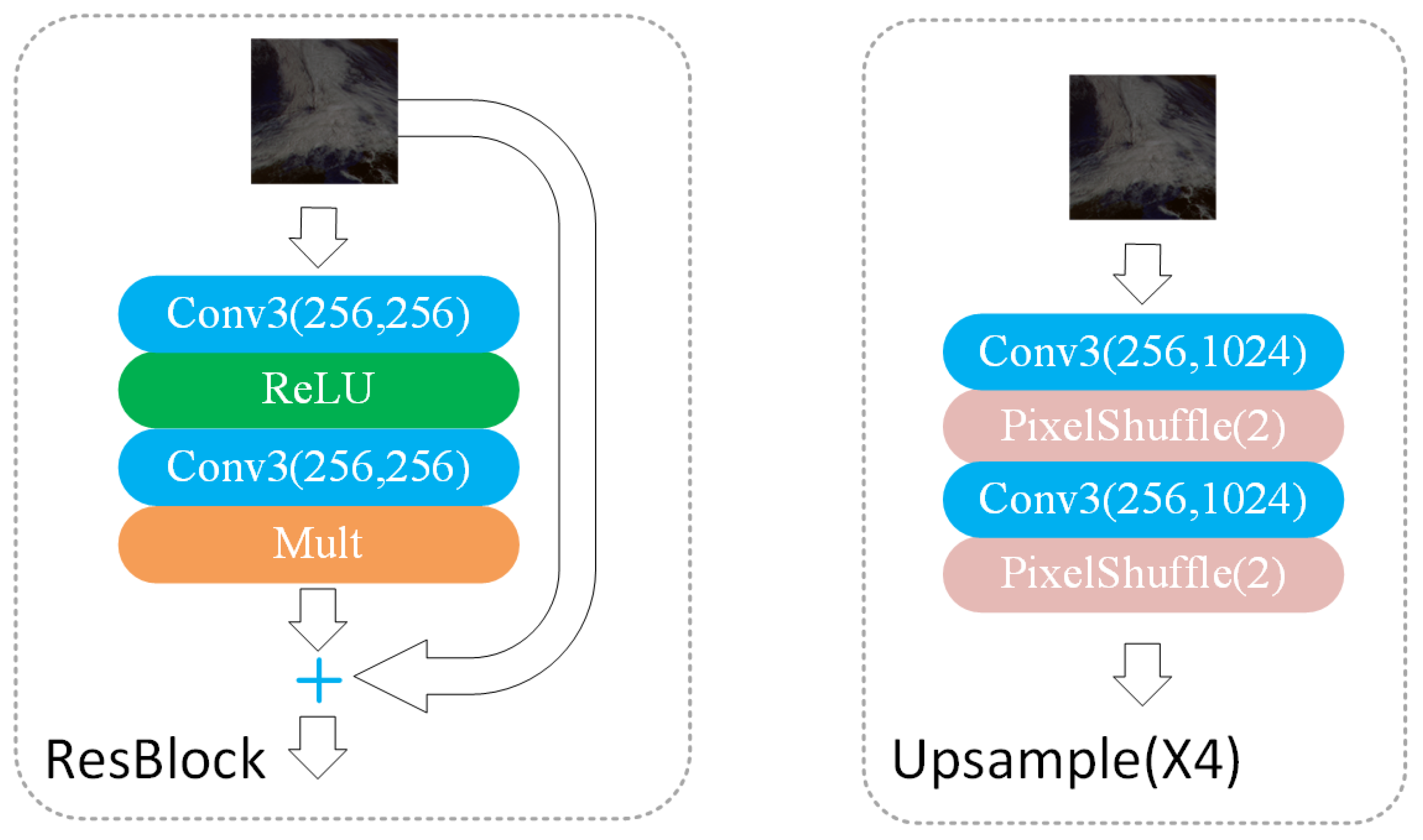
All the super-resolution algorithms for test were proposed in recent five years with deep neural networks modelling the upsampling process, as will be introduced in
Figure 3,
Figure 4,
Figure 5,
Figure 6,
Figure 7,
Figure 8,
Figure 9,
Figure 10 and
Figure 11. In these figures,
denotes that the channel numbers are
a for input and
b for output, conv3 denotes the
convolution, conv1 denotes the
convolution, FC denotes the fully connected layer, ReLU denotes the rectified linear unit for activation, and Mult denotes the multiplication operation.
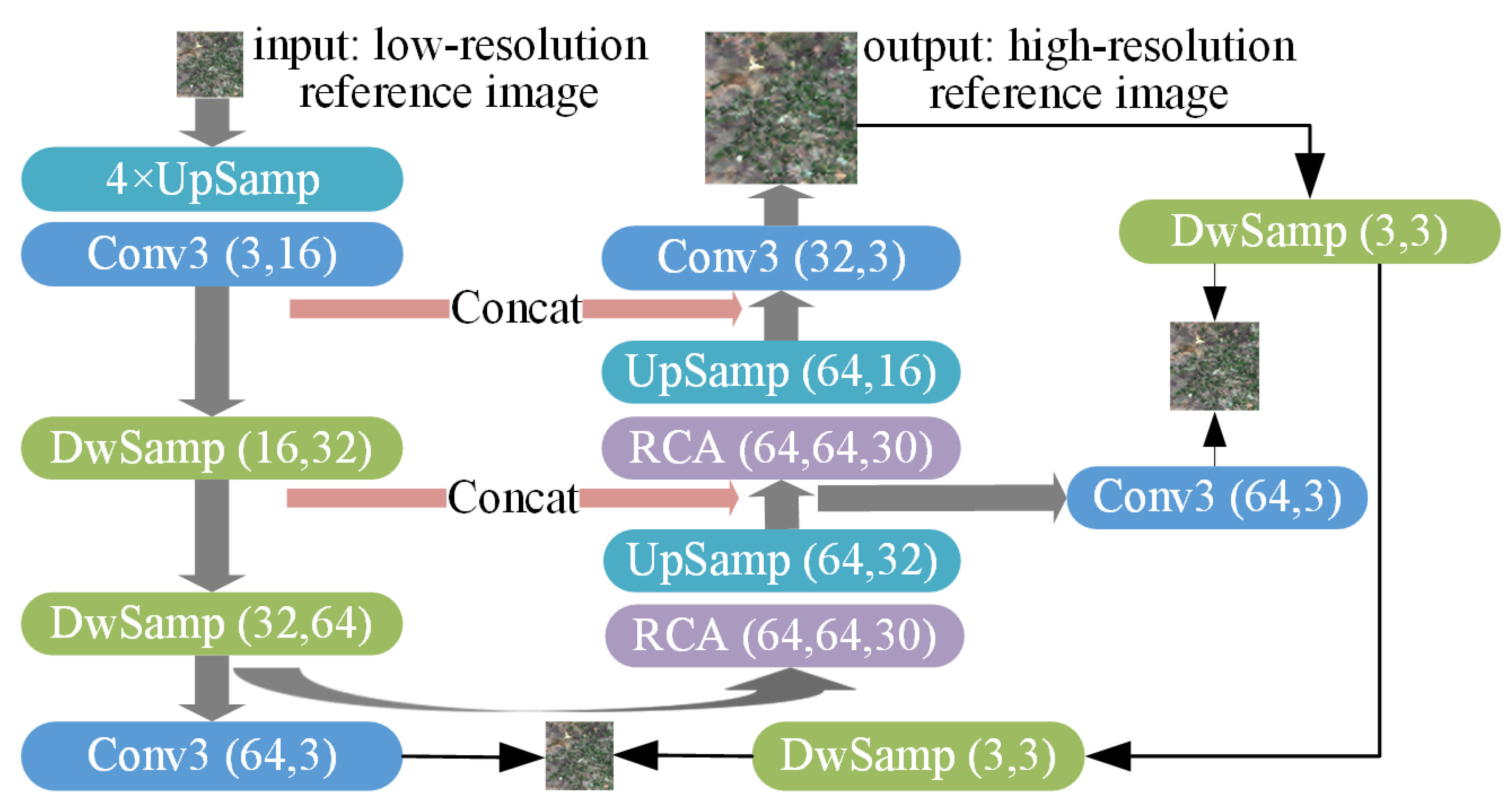
Ref. [
21] won the NTIRE2017 super-resolution challenge with the proposed enhanced deep residual networks (EDSR) by removing unnecessary modules in conventional residual networks. The structure and creative blocks of EDSR are presented in
Figure 3 and
Figure 4.
Ref. [
22] proposed the dual regression networks (DRN) for paired and unpaired super-resolution tasks. In DRN, an additional constraint is introduced on the low-resolution data to reduce the span space of possible solutions. A closed loop is designed with a feedback mapping to estimate the down-sampling kernel targeting the original low-resolution images. The structure and blocks of DRN are presented in
Figure 5 and
Figure 6.
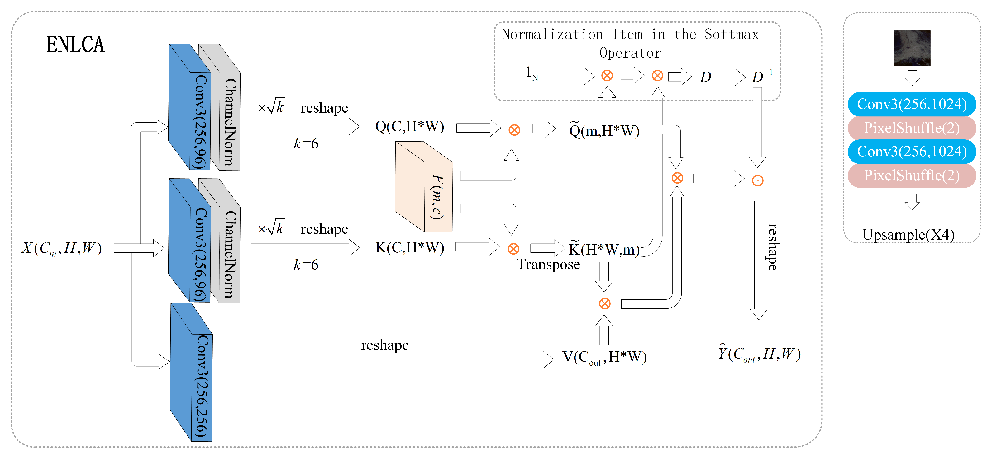
Ref. [
23] propose a new model with an efficient non-local contrastive attention (ENLCA) module to perform long-range visual modeling. The ENLCA module the leverage more relevant non-local features. The network structure is illustrated in
Figure 7, and the critical ENCLA module is in
Figure 8.
The concept of adaptive target is introduced in [
24] by generating from the original ground truth target with a transformation to match the output of the super-resolution network. To deal with the ill-posed nature of super-resolution, the adaptive target provides the flexibility of accepting a variety of valid solutions. Their adaptive target generator (AdaTarget) is an improvement to existing super-resolution networks. In [
24], ESRGAN is advised as the baseline super-resolution network (SR net in
Figure 9). In the PIRM2018-SR challenge, AdaTarget outweighed all the other super-resolution algorithms. The structure of AdaTarget is presented in
Figure 9.
Ref. [
25] proposed the scale-arbitrary super-resolution (ArbRCAN) network in the form of plug-in modules to enable existing super-resolution networks for scale-arbitrary super-resolution with a single model. ArbRCAN can be easily adapted to scale-specific networks with small additional computational and memory cost, which is very help for remote sensing images as sources may differ a lot. The structure and blocks of ArbRCAN are presented in
Figure 10 and
Figure 11, where the backbone network can be existing super-resolution network where EDSR was used in [
25].
3.2. Training and 16-bit Preprocessing
Two sets of model parameters are prepared for each dataset. All the methods were designed for natural images, and they have been trained with natural datasets, such as DIV2K or Flickr1024. Intuitively, we hope to know the performance of the model trained on natural image datasets and used for remote sensing images. On the other hand, an improvement in reconstruction accuracy is expected by training the model on a more matched dataset. The performance differences correspond to the migration ability of the models. Therefore, two experiments are designed using models either pre-trained on natural images or trained on proposed datasets. To accelerate the model training, the initial parameters for FY4ASRgray and FY4ASRcolor training are derived from the results of pre-training on natural images.
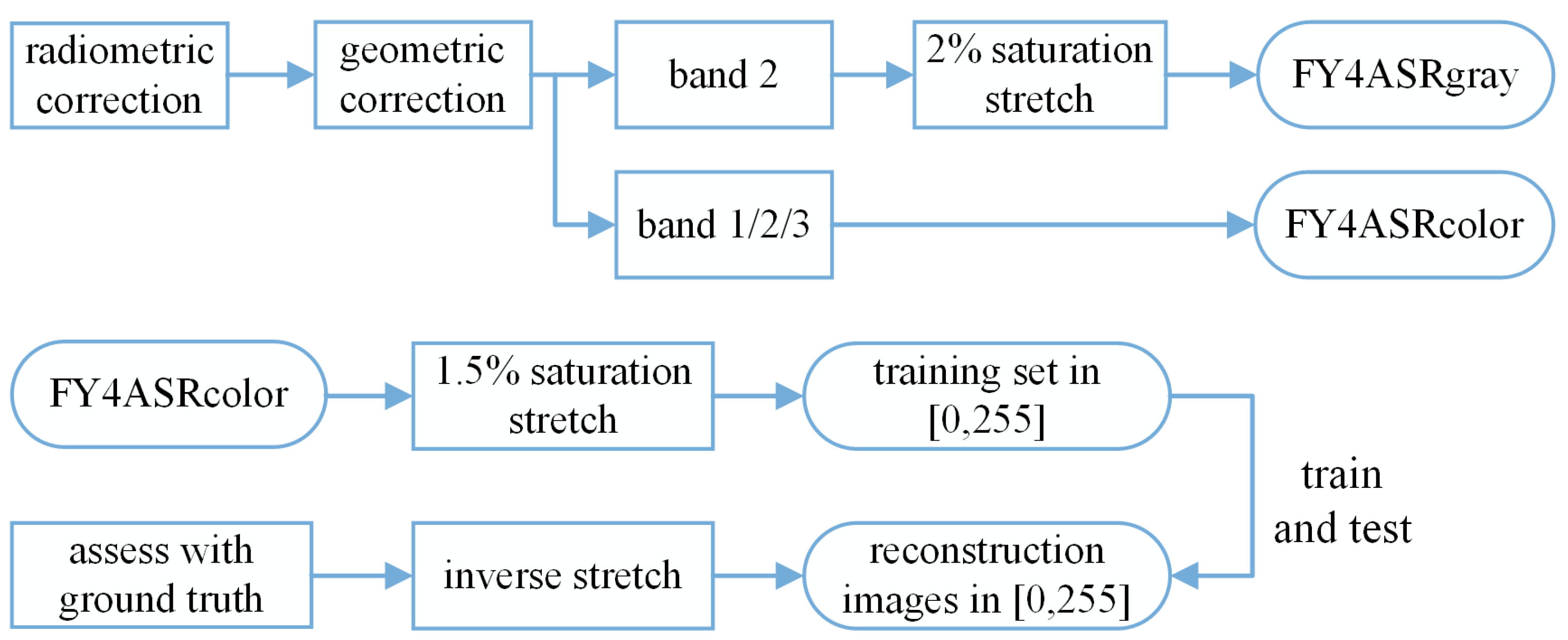
To test the FY4ASRcolor dataset with the natural image pre-trained models, the 16-bit quantization has to be dealt with. The pixel values of natural images usually range from 0 to 255. However, the FY4ASRcolor dataset is 16-bit quantized with the maximum value 4095, which cannot be tested directly using the pre-trained parameters. Due to outlier pixels, a linearly stretched remote sensing image is much too dark to maintain structural information. By approaching the style of training data, we propose to non-linearly stretch the pixel values in FY4ASRcolor with saturate thresholds. In the transformation, the values of the darkest 1.5% pixels are set to 0, and the values of the brightest 1.5% pixels are set to 255. The values of the remaining image pixels are linearly stretched to [0, 255] and recorded as floating point numbers. Stretched images can be put into the network for training and reconstruction. The reconstructed results should be linearly stretched back to [0, 4095] using the original thresholds defining the darkest and brightest 1.5% pixels. The forward stretch and backward stretch are performed band by band. Our tests show that a threshold of 1.5% allows the contrast of the image to be enhanced significantly without noticeable loss of radiometric fidelity. The full processing steps are demonstrated in
Figure 12.
For the FY4ASRgray dataset, after eliminating the surrounding invalid areas, the high-resolution image size was cropped to . By slicing the 1000 M resolution image into blocks, a total of 4662 image blocks were obtained, each with a low-resolution image block corresponding to it. Among the extracted image blocks, 4608 were used for training, 36 for validation, and 18 for testing.
As for the FY4ASRcolor dataset, the same block extraction strategy as FY4ASRgray was used after the 1.5% saturate stretch. Finally, we obtained 3057 pairs of image blocks. The size of high-resolution image blocks is , and the corresponding low-resolution size is . Among the extracted image blocks, 2507 are used for training, 270 for validation, and 280 for testing.
3.3. Metrics
Referenced metrics are used to assess the performance of the reconstructed images. Peak signal-to-noise ratio (PSNR), Root Mean Square Error (RMSE), and Correlated Coefficient (Corr) measure the radiometric discrepancy. Structural Similarity (SSIM) measures the structural similarity. Spectral angle mapper (SAM), relative average spectral error (RASE) [
26], relative dimensionless global error in synthesis (ERGAS) [
27], and Q4 [
28] measure the color consistency. The ideal results are 1 for SSIM, Corr, and Q4 while 0 for SAM, ERGAS, and RASE. The formulas for these metrics are listed below.
Two different PSNRs are calculated to deal with the various word lengths. For a FY4ASRgray reconstruction result, PSNR is calculated with . For FY4ASRcolor, PSNR is calculated with .
In addition to the full reference metrics, no-reference approaches [
29] are also introduced to assess image quality, including the Blind/Referenceless Image Spatial Quality Evaluator (BRISQUE) [
30], Naturalness Image Quality Evaluator (NIQE) [
31], and the Perception-based Image Quality Evaluator (PIQE) [
32]. Since these methods do not work properly on 16-bit data, they are only used on the FY4ASRgray test to calculate the no-reference image quality scores.
5. Discussion
The time of the images in the FY4ASRcolor dataset is on 16 September 2021 which starts at 00:30 and ends at 23:43. The acquisition duration of each image is 258 s. In terms of the time intervals of two adjacent images, most of them are 258 s, and the maximum value is 3084 s. The strong temporal continuity allows the data to be used for time-related studies. Therefore, two new experimental schemes were explored, namely sequence super-resolution and spatiotemporal fusion. The results of these studies are expected to uncover the feasibility of the new datasets for prediction of temporal correlation. An additional test is made to find the generalization ability. In these studies, only the FY4ASRcolor dataset is used as it better suits for the purpose of remote sensing.
5.1. Sequence Super-Resolution
We constructed a training set and a test set by considering the sequence images as a video, and performed a test of video super-resolution. To construct the training set, 40 various locations were selected. In total, 84 pairs of temporally consecutive patches were extracted from each location, which were divided into 12 groups in time order. Each group contains 7 pairs of temporally contiguous patches as a video clip for reconstruction. The patch sizes of each pair are and , cropped from the 1 km and 4 km images, respectively. After removing the groups with excessive darkness, 347 valid groups of video clips were finally obtained out of 480 groups of sequential images for training.
Similar to the training set, the test set was constructed to contain 10 groups of sequential patches at 10 various locations. These 10 locations are included in the 40 locations of the training set. Each group contains 10 pairs of temporally consecutive patches. The patch sizes of each pair are and , cropped from the 1 km and 4 km images, respectively. The 100 images used in the test set are beyond the training set.
The Zooming Slow-Mo algorithm [
33] is chosen to perform the sequence super-resolution, and its results are evaluated on the 100 test images. Only with the pre-trained model, the average PSNR is 28.2371 dB. With the pre-trained model as the initial value and the constructed dataset for re-training, the average PSNR is 29.2174 dB. When trained only with constructed training set where the pre-trained model is not used, the average PSNR is 30.1253 dB. By comparing these scores with that in
Table 3 and
Table 5, it is concluded that the gap between our FY4ASRcolor dataset and commonly used video sequence datasets is huge. To reconstruct sequence remote sensing images, both the a priori image structure and the sequence change pattern have to be learned, such that matching datasets is becoming difficult.
5.2. Spatiotemporal Fusion
Spatiotemporal fusion is a solution to enhance the temporal resolution of high spatial resolution satellites by exploiting the complementarity of spatial and temporal resolutions between satellite images of different sources. Typical studies are carried out between MODIS and Landsat satellites, which have revisit periods of 1 and 16 days, respectively. A typical spatiotemporal fusion needs three reference images. Assuming that MODIS captures images at moments and while Landsat took an image only at moment , spatiotemporal fusion algorithms try to predict the Landsat images at moment with the three known images.
The FY4ASRcolor dataset is ideal for conducting spatiotemporal fusion studies. Different from MODIS and Landsat, the two known images in the FY4ASRcolor dataset were taken at the exactly same time. They also have the same sensor response, which eliminates the fatal sensor discrepancy issue in fusing MODIS and Landsat. A similar work was carried out by us for the spatiotemporal-spectral fusion of the Gaofen-1 images [
17], but it has only a 2-fold difference in spatial resolution. The use of the FY4ASR dataset for spatiotemporal fusion may provide new fundamental data support for this research topic.
We try to use two methods for spatiotemporal fusion, namely FSDAF and SSTSTF [
16]. FSDAF is a classical algorithm, while SSTSTF is one of the latest algorithms based on neural networks. SSTSTF requires large amount of data for training, otherwise the performance is not as good as FSDAF. However, FSDAF fails in our test because it cannot give legible images. The changing sunshine intensities lead to a huge variation in the reflection of the features, which may exceed the temporal difference tolerance that FSDAF can reconstruct for surface reflectance. In contrast, SSTSTF can accomplish the reconstruction successfully.
For SSTSTF, paired images from 12 moments were used to construct the dataset. Each high-resolution image has a size of . Images from 9 moments were used for training, and they formed 8 groups. The test used images from 3 other moments, two of which were set as the prediction time. The reconstruction PSNRs are 32.9605 dB for 6:30 and 36.8904 dB for 11:30, respectively, after removing the dark areas from the reconstructed images as it may elevate PSNR values unfairly. The results show that the reconstruction quality of spatiotemporal fusion is weakly less than that of single-image super-resolution. Considering that the amount of training data is far smaller than that used for training of single-image super-resolution, spatiotemporal fusion algorithms need to be carefully designed to adapt to this new dataset.
5.3. Generalization of Trained Models across Datasets
In order to evaluate the generalization of the model trained based on the FY4ASRcolor dataset for remote sensing, it is planned to apply the trained models to other datasets. Unfortunately, the existing studies use images with ultra-high resolutions, which prevents us from finding matching application scenarios. Finally, the datasets used in [
34] were tested. Two datasets were involved in the experiment, the 0.3 m UC Merced dataset and the 30 m to 0.2 m NWPU-RESISC45 dataset. The tested images are denseresident191 in the UC Merced dataset and railwaystation565 in the NWPU-RESISC45 dataset. The scores of PSNR evaluation are listed in
Table 8 where the bolded numbers highlight the best scores across algorithms. The results from pre-training models are close to the values in [
34]. However, re-training on FY4ASRcolor leads to a substantial decrease in reconstructing high-resolution remote sensing images. This convinces us again that the characteristics of our data are quite different from other datasets. This conclusion is easily concluded, as meteorological satellite images have to lose spatial resolution to ensure high temporal resolution. Knowledge of structural details cannot be learned from low-resolution images to reconstruct complex structures of high-resolution images. On the contrary, the temporal repetition and spectral features play much greater roles in the reconstruction process.
