Forest Fire Occurrence Prediction in China Based on Machine Learning Methods

Abstract

Forest fires may have devastating consequences for the environment and for human lives. The prediction of forest fires is vital for preventing their occurrence. Currently, there are fewer studies on the prediction of forest fires over longer time scales in China. This is due to the difficulty of forecasting forest fires. There are many factors that have an impact on the occurrence of forest fires. The specific contribution of each factor to the occurrence of forest fires is not clear when using conventional analyses. In this study, we leveraged the excellent performance of artificial intelligence algorithms in fusing data from multiple sources (e.g., fire hotspots, meteorological conditions, terrain, vegetation, and socioeconomic data collected from 2003 to 2016). We have tested several algorithms and, finally, four algorithms were selected for formal data processing. There were an artificial neural network, a radial basis function network, a support-vector machine, and a random forest to identify thirteen major drivers of forest fires in China. The models were evaluated using the five performance indicators of accuracy, precision, recall, f1 value, and area under the curve. We obtained the probability of forest fire occurrence in each province of China using the optimal model. Moreover, the spatial distribution of high-to-low forest fire-prone areas was mapped. The results showed that the prediction accuracies of the four forest fire prediction models were between 75.8% and 89.2%, and the area under the curve (AUC) values were between 0.840 and 0.960. The random forest model had the highest accuracy (89.2%) and AUC value (0.96). It was determined as the best performance model in this study. The prediction results indicate that the areas with high incidences of forest fires are mainly concentrated in north-eastern China (Heilongjiang Province and northern Inner Mongolia Autonomous Region) and south-eastern China (including Fujian Province and Jiangxi Province). In areas at high risk of forest fire, management departments should improve forest fire prevention and control by establishing watch towers and using other monitoring equipment. This study helped in understanding the main drivers of forest fires in China over the period between 2003 and 2016, and determined the best performance model. The spatial distribution of high-to-low forest fire-prone areas maps were produced in order to depict the comprehensive views of China’s forest fire risks in each province. They were expected to form a scientific basis for helping the decision-making of China’s forest fire prevention authorities.

1. Introduction

Forest fire disaster is considered one of the leading causes of dramatic depletion of forest ecosystems worldwide among either anthropogenic or natural processes [1,2]. From 2003 to 2018 years, there were 111,446 forest fire disasters in China, and the total area of forest fires nationwide was 3,289,500 hm², with an average annual fire area of 205,600 hm² [3]. Extreme fire weather conditions have become more common globally due to global warming and extended fire weather seasons in recent decades, enhancing the flammability of vegetation and preparing many landscapes for more frequent burning. Forest fires are becoming even more pronounced within fire regimes in many regions, with increasing impacts on human survival environment and ecosystem function processes [4]. Fire regimes are shaped by climate, landscape structure, and the frequency of ignitions and vary globally across space, biogeographies, and environments. Fire regimes are also strongly sensitive to human activities and global change drivers, and have strong impacts on ecosystems, biodiversity and societies. Thus, forest fire prevention has become a key research topic in forestry and ecology, development of reliable prediction models of forest fire danger is important for public safety, forest management, and suppression planning [5,6,7,8,9,10].

By establishing a forest fire prediction model, we can predict the probability of the occurrence of a forest fire and then manage the area where the fire is likely to occur.Various models have been proposed for forest fire danger prediction, varying from simple statistical techniques (i.e., Poisson regression, geographically weighted regression, logistic regression) to more complex models (i.e., Pareto distribution, favorability functions, and approaches based on numerical simulation) [11,12,13,14,15,16,17,18,19,20]. Liao et al. (2008) used the zero-inflated Poisson model to predict the frequency of forest fires in Japan in 2000 [21]. Guo et al. (2010) used ordinary least squares regression, zero-inflated negative binomial model to predict the number of forest fires in the Greater Xing’an Mountains area of Heilongjiang Province, China [22]. MAXENT has also been applied to various hazard risk assessments, such as landslides, wildfires, and pandemics. Massada et al. (2013) argued that a presence–absence modeling approach may be more suitable in areas with long-term fire records and where only a small part of the area can sustain a fire. MaxEnt is able to cope well with sparsely, irregularly sampled data and minor location errors [23,24,25]. However, a forest fire is typical a nonlinear and complex process that is governed by many influencing factors [26,27,28]. Therefore, it is challenging to model and predict the occurrence of forest fires [29,30].

In recent years, machine learning has been employed for deep analysis and mining of information in environmental variables for forest fire prediction such as neural networks, support vector machines, random forests, logistic regression classifiers with kernel function, and neural fuzzy models [31,32,33,34,35]. The common conclusion from the above researches is that machine learning models have proven abilities to deliver better results [36,37]. In those machine learning models, artificial neural networks (ANNs) consist of neurons with adjustable connection weights. Unlike traditional multiple linear or parametric regression models, neural networks have better self-organization and self-learning capabilities, and they have been widely used in forest fire prediction [38,39]. For example, Maeda et al. (2009) used ANNs and multitemporal images from MODIS/Terra-Aqua sensors to detect areas at high risk of forest fires in Brazil’s Amazon region [40]. The results showed that the error was small, and the predictions were accurate. Sakr et al. (2011) predicted the occurrence of forest fires in developing countries through two meteorological factors using artificial neural networks [41]. A radial basis function (RBF) neural network is a three-layer neural network, a particular case of a back-propagation neural network. Little research has used RBF neural networks for forest fire prediction. Samaher (2018) used an RBF neural network to predict the forest fire risk in natural parks in Portugal [26]. Support-vector machines (SVMs) are most suitable for the binary classification of data in the form of supervised learning. SVMs apply the principle of structural risk minimization and have good learning abilities. Researchers have recently started using SVMs to predict forest fires [42,43,44]. Samaher (2018) used five different soft computing (SC) technologies, including an SVM algorithm, to predict areas at risk of forest fires [26]. He determined that the SVM algorithm provides more accurate predictions than the other four. Cortez et al. (2007) used five different data mining (DM) algorithms to predict the area at risk of forest fires in the north-eastern region of Portugal [8]. Their results showed that the prediction effect of the model was good. Based on Cortez’s research, Xu et al. (2012) used the semidefinite programming model to select the optimal kernel function of the SVM to establish an SVM model for forest fire prediction [7]. The mean square error was small, and the model effect was good. The random forest (RF) algorithm is a well-known integrated learning algorithm that can provide higher accuracy than other algorithms. Currently the use of RFs to predict forest fires is relatively established [45,46,47]. Liang et al. (2016) used an RF model to predict the occurrence of forest fires in Fujian Province, China, with an accuracy rate of 85% [48]. Pourtaghi et al. (2016) used an RF algorithm to study the sensitivity of forest fires in Golestan Province, Iran, and their results showed that the model achieved the desired accuracy [49]. It is debated which method or technique is the best for modeling forest fires. Therefore, comparison of methods and techniques is highly necessary to gather reasonable conclusions for forest fire prediction [44].

Most of the current studies have focused on some specific regions, while few studies have been conducted to forecast and analyze the whole range of long time scales in China. Many studies have concentrated on the temporal and spatial changes and influencing factors of forest fires in specific years [50,51,52,53]. The results of previous research are therefore localized and limited, and there is a lack of studies investigating the most suitable and high-precision forest fire prediction model on the national scale.

Compared to studies on the local level, we performed a national-scale forest fire occurrence prediction in China, while considering the problem of forest fires over longer time scales. We selected a variety of forest fire drivers, built four prediction models based on machine learning algorithms, and evaluated the models using Chinese forest fire data collected from satellite remote sensing monitoring for a total of 14 years from 2003 to 2016. The study has three objectives: (1) identify the primary central forest fire driving factors and their impacts in China; (2) select the most suitable model for forest fire prediction in China by creating four models and comparing and analysing the fitting results; and (3) use the model that offers the most accurate predictions to create a forest fire probability map for China and put forward recommendations for forest fire prevention.

2. Materials and Methods

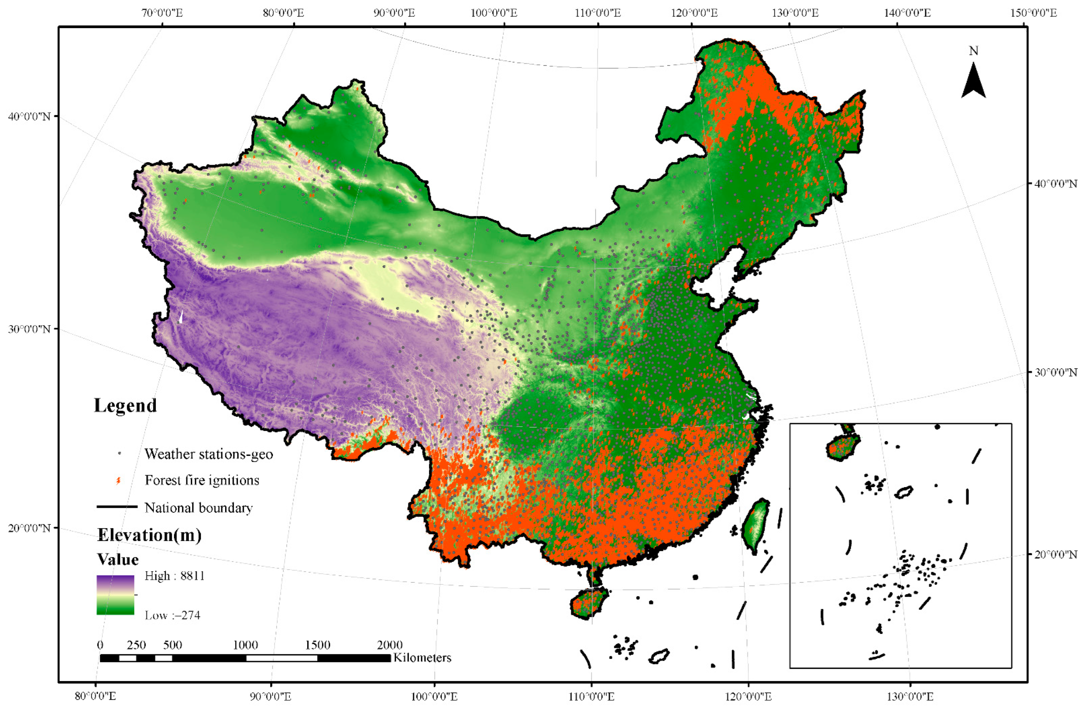
2.1. Study Area and Data Resources

China is located in East Asia on the west coast of the Pacific Ocean and has a vast territory with a total land area of about 9.6 million square kilometers. The topography is high in the west and low in the east, with large mountainous areas and plateaus. The distance between the east and west of the country is about 5000 km, the continent has a coastline of more than 18,000 km, and a variety of temperatures and precipitation that create a variety of climates. China’s forest resources are unevenly distributed, mainly in Northeast, South China, and Southwest China. The forest land area is 220 million hectares, and the forest coverage rate is 22.96%.

The research data had six parts: fire ignition data, meteorological data, terrain data, vegetation data, infrastructure data, and socioeconomic data [5]. The fire points data were derived from NASA’s Global Fire Atlas with Characteristics of Individual Fires, 2003–2016 (https://daac.ornl.gov/ (accessed on 1 January 2021)). The Global Fire Atlas is a global dataset that tracks the daily dynamics of single fires. For each fire, the dataset provides information about the fire’s timing and location, scale, perimeter, duration, speed, and direction of spread. These unique fire characteristics are based on the Global Fire Atlas algorithms and estimated combustion day information from a 500-m resolution product of the six MCD64A1 combustion zone products of the Medium Resolution Imaging Spectroradiometer (MODIS) collection.

This study used fire point data for forest land in China from 2003 to 2016. The final number of fire points was 32,746 (excluding Taiwan). The meteorological data were derived from the 14-day daily value dataset of the China Meteorological Data Network (http://data.cma.cn/dataService/ (accessed on 7 January 2021). The dataset includes eight elements, such as barometric pressure, temperature, relative humidity, and precipitation at the station. Digital elevation model (DEM) data were obtained through Data Center for Resources and Environmental Sciences, Chinese Academy of Sciences (https://www.resdc.cn/ (accessed on 10 January 2021)). Vegetation data were represented by the normalized difference vegetation index (NDVI), and the spatial distribution dataset of China’s Quarterly Vegetation Index came from the Resource and Environment Data Cloud Platform (http://www.resdc.cn/ (accessed on 10 January 2021). The primary geographic data were taken from the “National Basic Geographic Database of 1:1 Million” website of the National Geographic Information Resources Directory System (http://www.webmap.cn (accessed on 13 January 2021)). The data include the locations of railways, highways, water systems, and residential areas. The socioeconomic data include population density and GDP per capita, and the grid data of the spatial distribution of population and GDP were obtained from the Resource and Environment Data Cloud Platform (https://www.resdc.cn/ (accessed on 15 January 2021)). Figure 1 shows the map of the study area.

2.2. Data Pre-Processing

2.2.1. Variable Handling

The dependent variable was a binary variable (i.e., whether or not a forest fire occurs). Thus, we used ArcGIS 10.4 to create a certain percentage of random points (non-fire points) and assigned a value of 1 to fire points and a value of 0 to non-fire points [54]. To ensure that the data were not over dispersed, random points were selected according to experience in a ratio of 1:1 [55]; in principle, randomness in space and time should be followed [56]. We used ArcGIS 10.4 software to create random points to ensure that fall on forest land, so the national land use data (http://www.dsac.cn/ (accessed on 10 January 2021) from 2003 to 2015 is used as the basis for the range of forest land extracted and the random points are created within that range to exclude random points located in bodies of water or urban land. We obtained a total of 65,492 fire points and random points.

For the meteorological data, we first used ArcGIS 10.4 to match the sample points with the nearest meteorological station. We then extracted the corresponding sample point weather data and used an SQL server database to match the daily weather data. For the terrain data, we used the spatial analysis tool in ArcGIS 10.4 to extract the slope and aspect of the obtained DEM data [57,58,59]. Seasonal climatic differences have an impact on vegetation status, we divided the year into spring (March, April, May), summer (June, July, August), autumn (September, October, November), and winter (December, January, February) [60]. We used the extraction and analysis tools of ArcGIS to extract the NDVI data for the sample points on an annual basis and quarterly basis.

Similarly, from the infrastructure data and socioeconomic data, we extracted the information corresponding to the sample points. We set the aspect and unique festivals as categorical variables and the others as continuous variables.

Table 1. Descriptions of aspect classifications.

Aspect	Azimuth (Degree)	Classification
Gentle Slope	−1	0
Shady Slope	0~67.5, 337.5~360	1
Semi-shady Slope	67.5~112.5, 292.5~337.5	2
Sunny Slope	157.5~247.5	3
Semi-sunny Slope	112.5~157.5, 247.5~292.5	4

shows the classification of aspect. During specific traditional celebrations in China, people burn the paper to commemorate their loved ones, increasing the probability of a forest fire. We classified (value 1) the following dates of these events as special festivals: Chinese New Year’s Eve, the first day of the first lunar month, the second day of the first lunar month, the fifteenth day of the first lunar month, and Qingming Festival and Zhongyuan Festival (15th July of the lunar calendar). Non-special festivals were set to 0.

After processing, we obtained 20 independent variables and their possible values (see

Table 2. Descriptions of independent variables.

Category	Independent Variable	Symbol	Variable Type	Source	Resolution, Units
Location	Longitude (°)	Lon	Continuous Variable	https://daac.ornl.gov/ (accessed on 1 January 2021)	-
	Latitude (°)	Lat	Continuous Variable	https://daac.ornl.gov/ (accessed on 1 January 2021)	-
Topographic	Altitude (m)	Alt	Continuous Variable	https://www.resdc.cn (accessed on 10 January 2021)	1 km
	Slope (°)	Slo	Continuous Variable	https://www.resdc.cn (accessed on 10 January 2021)	1 km
	Aspect	Asp	Categorical Variable	https://www.resdc.cn (accessed on 10 January 2021)	1 km
Climatic	Average Surface Temperature (°C)	Avst	Continuous Variable	China Ground Climate Da ta(V3.0) Daily Dataset, National Meteorological Information Centre (https://data.cma.cn (accessed on 7 January 2021)	0.1 °C
	Daily Maximum Surface temperature (°C)	Mast	Continuous Variable		0.1 °C
	Cumulative Precipitation at 20–20 (mm)	Pre	Continuous Variable		0.1 mm
	Average Relative Humidity (%)	Arh	Continuous Variable		1%
	Hours of Sunshine (h)	Suh	Continuous Variable		0.1 h
	Average Temperature (°C)	Ate	Continuous Variable		0.1 °C
	Daily Maximum Temperature (°C)	Mate	Continuous Variable		0.1 °C
	Average Wind Speed (m/s)	Aws	Continuous Variable		0.1 m/s
	Maximum Wind Speed (m/s)	Mws	Continuous Variable		0.1 m/s
Infrastructure	Distance from Fire Point to Highway (m)	Hig	Continuous Variable	https://www.webmap.cn (accessed on 13 January 2021)	1:1,000,000
	Closest Distance from Fire Point to Residential Area (m)	Set	Continuous Variable	https://www.webmap.cn (accessed on 13 January 2021)	1:1,000,000
Socioeconomic	Population	Pop	Continuous Variable	https://www.resdc.cn (accessed on 15 January 2021)	1 km
	GDP	GDP	Continuous Variable	https://www.resdc.cn (accessed on 15 January 2021)	1 km
	Special Festival	Sfe	Categorical Variable	-	-
Vegetation	NDVI	NDVI	Continuous Variable	https://www.resdc.cn (accessed on 10 January 2021)	1 km

). Finally, we performed data cleaning on the sample points and the various types of data extracted to remove abnormal samples from the original dataset (including some samples with missing data and models with observations that were significantly outside the normal range).

2.2.2. Data Normalization

Given the different dimensions and magnitudes of the factors above, the data were normalized to eliminate the variation in dimensions, avoid significant differences in the volumes of the input and output data, and balance the contributions of various factors. All data were converted to values between 0 and 1.

Table 3. Normalized formulas and explanations.

No.	Formula	Explanation	Variables Using This Formula
(1)	${\mathrm{x}}_{\mathrm{i}}{}^{*}=\frac{{\mathrm{x}}_{\mathrm{i}}-{\mathrm{x}}_{\min }}{{\mathrm{x}}_{\max }-{\mathrm{x}}_{\min }}$	${\mathrm{x}}_{\mathrm{i}}$ and ${\mathrm{x}}_{\mathrm{i}}{}^{*}$ are the values before and after data normalization, respectively;${ \mathrm{x}}_{\max }$ and ${\mathrm{x}}_{\min }$ are the maximum and minimum values of the full sample data, respectively.	Lon, Lat, Alt, Avst, Mast, Pre, Suh, Ate, Mate, Aws, Mws, Hig, Set, Pop, GDP
(2)	${\mathrm{x}}_{\mathsf{\alpha }}=\sin \mathsf{\alpha }$	$\mathsf{\alpha }$ is the slope value.	Slo
(3)	${\mathrm{x}}_{\mathsf{\gamma }}=\frac{\mathsf{\gamma }}{100}$	$\mathsf{\gamma }$ is the humidity value.	Arh

shows the normalized formulas and specific interpretations of the independent variables.

2.3. Method

In this study, we used the MATLAB and R Studio programming languages to implement the algorithms. We used MATLAB to build the ANN, RBFNN, and SVM models and used R Studio to build the RF models.

This study provides a methodological framework for predicting the occurrence of forest fires in China, as shown in Figure 2. First, all of the forest fire correlation factors are selected by feature selection to obtain the forest fire driving factors that have significant influence on fires. These factors are then used as input data of the forest fire prediction model, and machine learning models (ANNs, RBF neural networks, SVMs and RFs) are applied to obtain corresponding results. Finally, the model accuracy is obtained through evaluation indexes such as the AUC value.

2.3.1. Artificial Neural Networks

ANNs have become widely used in feedforward networks due to their clear structure, fast operation, easy implementation, and abilities for self-learning and adaption to the environment [57,58]. ANNs consist of three parts: an input layer, an output layer, and a hidden layer. The hidden layer may be a topological structure of one or more layers. The input layer does not perform any calculations; rather, it is used to receive data, that is, to transfer data to the adjacent hidden layer with different weights. The hidden layer processes the data through a nonlinear activation function and then passes it to the output layer. The final result is obtained from the output layer. The mathematical principle is as follows:

$$\{\begin{array}{c}{\mathrm{h}}^{\left(1\right)}={\mathsf{\phi }}^{\left(1\right)}({{\displaystyle \sum }}_{\mathrm{i}=1}^{\mathrm{n}}{\mathrm{x}}_{\mathrm{i}}·{{\mathsf{\omega }}_{\mathrm{j}}}^{\left(1\right)}+{\mathrm{b}}^{\left(1\right)}\\ \mathrm{y}={\mathsf{\phi }}^{\left(2\right)}({{\displaystyle \sum }}_{\mathrm{j}=1}^{\mathrm{n}}{{\mathrm{h}}_{\mathrm{i}}}^{\left(1\right)}·{{\mathsf{\omega }}_{\mathrm{j}}}^{\left(2\right)}+{\mathrm{b}}^{\left(2\right)}\end{array}$$

(1)

In the formula, the input layer is $\mathrm{x}\in R^m$, the hidden layer output is $\mathrm{h}\in R^n$, the output layer is $\mathrm{y}\in R^K$, the input layer to the hidden layer weight confourection matrix is ${\mathsf{\omega }}^{\left(1\right)}\in R^{m\times n}$, the weight connection bias from the input layer to the hidden layer is ${\mathrm{b}}^{\left(1\right)}\in R^n$, and the weight connection matrix and the bias from the hidden layer to the output layer are ${\mathsf{\omega }}^{\left(2\right)}\in R^{n\times K}$ and ${\mathrm{b}}^{\left(2\right)}\in R^{n\times K}$, respectively.

2.3.2. Radial Basis Function Neural Network

The RBF neural network structure is a feedforward structure with an input layer, a single hidden layer, and an output layer. Its advantages are concise training and fast learning convergence speed, which can approximate any nonlinear function. This method has been widely used in time-series forecasting, nonlinear control systems, and the graphics-processing field. The basic idea of an RBF neural network is as follows. The RBF is used as the “base” of the hidden unit to form the hidden layer space. The hidden layer transforms the input vector and the low-dimensional pattern input data into the high-dimensional space. The result is that the data are linearly separable in the high-dimensional area. The output of the RBF neural network is as follows:

$${\mathrm{y}}_{\mathrm{i}}={{\displaystyle \sum }}_{\mathrm{i}=1}^{\mathrm{h}}{\mathsf{\omega }}_{\mathrm{ij}}\exp \left(-\frac{1}{2{\mathsf{\sigma }}^2}\Vert {\mathrm{x}}_{\mathrm{p}}-{\mathrm{c}}_{\mathrm{i}}\Vert {}^2\right) \mathrm{j}=1,2,\cdots ,\mathrm{n}$$

(2)

where ${\mathrm{x}}_{\mathrm{p}}={\left({x_1}^p,{x_2}^p,\cdots ,{x_m}^p\right)}^T$ is the pth input sample (p = 1,2,3,…,P), P is the total number of samples, ${\mathrm{c}}_{\mathrm{i}}$ is the centre of the hidden layer node of the network, ${\mathsf{\omega }}_{\mathrm{ij}}$ is the connection weight from the hidden layer to the output layer, i = 1,2,3,…,h is the number of hidden layer nodes, and ${\mathrm{y}}_{\mathrm{i}}$ is the actual output of the jth output node of the network corresponding to the input sample [59].

2.3.3. Support-Vector Machines

SVMs are mainly used for pattern classification and nonlinear regression. They are general learning algorithms based on the principle of structural risk minimization. The core idea of an SVM is to establish a classification hyperplane as a decision surface to maximize the isolation edge between the positive and negative examples, thereby providing a high generalization performance [60]. SVMs can improve the ability to transform data from high-dimensional spaces by flexibly using kernel functions when dealing with various nonlinear problems. Taking a two-class SVM as an example, given a training set $T=\left\{\left(x_1,y_1\right),\cdots \left(x_l,y_l\right)\right\}\in {\left(X\times Y\right)}^l$, where $x_i\in X=R^n, y_i\in \left\{1,-1\right\}\left(i=1,2,\cdots l\right)$, $x_i$ is the feature vector. The penalty parameter C and the kernel function $K\left(x,x^{\prime }\right)$ are first selected, and the optimization problem is then constructed and solved as follows [59]:

$$\underset{\alpha }{\min }\frac{1}{2}{{\displaystyle \sum }}_{i=1}^j{{\displaystyle \sum }}_{j=1}^l{y}_i{y}_j{a}_i{a}_{j}K\left(x,x^{\prime }\right)-{{\displaystyle \sum }}_{j=1}^l{\alpha }_j$$

(3)

$$s.t. {{\displaystyle \sum }}_{i=1}^l{y}_i{\alpha }_i=0, 0\le {\alpha }_i\le C,i=1,\cdots ,l$$

(4)

The optimal solution is then obtained: ${\alpha }^{*}={\left({\alpha }_1{}^{*},\cdots ,{\alpha }_l{}^{*}\right)}^T$. A positive component of ${\alpha }^{*}$: $0\le {\alpha }_j{}^{*}\le C$ is then selected, and the threshold is calculated as follows:

$$b^{*}=y_j-{{\displaystyle \sum }}_{i=1}^l{y}_i{{\alpha }_i}^{·}K\left(x_i-x_j\right)$$

(5)

Finally, the decision function is constructed:

$$f\left(x\right)=sgn({{\displaystyle \sum }}_{i=1}^l{{\alpha }_i}^{*}{y}_{i}K\left(x,x_i\right)+b^{*}$$

(6)

2.3.4. Feature Selection and Random Forest

Feature selection refers to the choice of subsets from the original feature set to optimize a certain evaluation criterion so that the model established with the optimal feature subset can achieve a prediction accuracy similar to or better than that of the model shown without feature selection [61,62]. RFs have been demonstrated to have a high prediction accuracy high tolerance to outliers and ’noise’ [63]. This method can be used to evaluate the relationship between covariates and dependent variables and calculate the relative importance of covariates [64,65]. RF has been applied in various fields, including medicine, genetics, ecology, and remote sensing. In recent years, it has been widely used in forest fire prediction and has demonstrated good predictive abilities [2,4]. The order of importance of variables can be obtained by a random forest algorithm. In previous studies, the variables screened by this method have been proved to have high reliability [4,23,66,67,68,69]. Therefore, the random forest algorithm is selected as the method of feature selection in this study. The basic idea of feature selection using RF is as follows: for the jth variable ($X_j$), the OOB error ($errOO{B}^j{}_t$) of each tree t is calculated, and then the value of the jth variable ($X_j$) is permuted while all others are left unchanged among OOB data, and the OOB error ($errOO{B}^j{}_t$) is again recalculated on this permuted dataset. RF estimates the importance of a variable by evaluating how much the prediction error increases when the OOB data for that variable are permuted. The importance score of $X_j$ is as follows:

$$VI\left(X^j\right)=\frac{1}{ntree}{{\displaystyle \sum }}_t\left(er{r}^{\prime }OO{B^j}_t-errOO{B}_t\right)$$

(7)

where R is the summation of all of the trees, and ntree is the number of trees in the RF [70,71]. For classification, the OOB is the misclassification probability.

An RF is a highly flexible machine learning algorithm with broad application prospects. An RF is a classifier consisting of multiple DTs formed by random methods. These trees are not related, hence its alternative name: “random decision tree”. When the test data enter the RF, each DT is classified, and the category with the most classification results among all of the DTs is taken as the final result.

The basic principle of the RF algorithm is as follows. Let N be the number of attributes of the sample. n is an integer greater than 0 and less than N. First, the bootstrap method is used for resampling, randomly generating M training sets S1, S2, … SM. DTs A1, A2,…AM corresponding to each training set is then generated. Before selecting the attribute in each non-leaf node, n attributes are randomly chosen from the N attributes as the split attribute set of the current node, and the node is split in the best split mode among the n attributes. Each tree grows intact without pruning. For the test set sample X, each DT is used to test and obtain the corresponding categories: C1(X), C2(X),…, CM(X). Finally, the voting method is adopted, and the category with the most output among the M DTs is regarded as the category to which the test set sample X belongs [59].

2.3.5. Model Performance Evaluation

In this study, we used five performance indicators (accuracy, precision, recall, f1 value, and AUC) to evaluate the performance of the models. Descriptions of the five indicators are given below.

1. Accuracy: the proportion of the number of samples (TP and TN) that are correctly predicted to the total number of samples. The formula is as follows:

$$P=\frac{TP+TN}{TP+FP+TN+FN}$$

(8)

2. Precision: characterizes the classification effect of the classifier, which is the correct frequency value predicted in the instance of the positive sample:

$$T=\frac{TP}{TP+FP}$$

(9)

3. Recall: characterizes the recall effect of a particular class. It is the correct frequency of prediction in the instance of the label as the positive sample:

$$R=\frac{TP}{TP+FN}$$

(10)

4. f1 value: the value used to measure precision and recall. It is the harmonic mean of these two values:

$$\mathrm{f}1=\frac{2TP}{2TP+FP+FN}$$

(11)

5. A receiver operating characteristic (ROC) curve is a method used to judge the prediction effect of the model [60]. The prediction accuracy of the model is judged by the value of the AUC, which ranges from 0.5 to 1. The larger the value, the closer the model’s fit is.

Note: TP, FN, FP, and TN in the formulas are the labels of the confusion matrix form of the output result.

3. Results

To evaluate feature factors and model performance issues, the dataset was divided into two parts by randomly selecting 70% of the pre-processed sample data as the training set and 30% as the test set [58].

3.1. Feature Selection

We used the RF algorithm to select the features of all variables after pre-treatment and select the subset of features that had the most significant impact on the dependent variables for the next model construction process. We divided the whole sample according to the above proportion (70% to the training set and 30% to the test set) and repeated this process five times in order to obtain five training samples [5]. Then, the varSelRF package in the R language was used to select and calculate the characteristic variables of the five training samples to obtain the variable subsets of the five intermediate models, and the variables appearing more than three times in the five variable quantum sets were selected as the variables after screening. The results are shown in

Table 4. Results of variable selection based on RF.

No.	Variable	Sample 1	Sample 2	Sample 3	Sample 4	Sample 5	Frequency
1	Lat	+	+	+	+	+	5
2	Lon	+	+	+	+	+	5
3	Avst	+	+	+	+	+	5
4	Mast	+	+		+	+	4
5	Pre	+	+		+	+	4
6	Arh	+	+	+	+	+	5
7	Suh	+	+	+	+	+	5
8	Ate	+	+	+	+	+	5
9	Mate	+	+	+	+	+	5
10	Aws						0
11	Mws						0
12	Alt	+	+	+	+	+	5
13	Slo						0
14	Asp						0
15	Set						0
16	Hig						0
17	GDP	+	+		+	+	5
18	Pop	+	+	+	+	+	5
19	NDVI	+	+	+	+	+	5
20	Sfe						0

. All variables and variables filtered by feature selection were used as input data for RF modeling, and the out-of-pocket error rate (OOB) and confusion matrix were obtained, as shown in

Table 5. The results of the OOB and confusion matrix of the two samples.

Total Variable Sample	OOB Estimate of Error Rate		10.89%
Confusion matrix:	0	1	Classification error rate
0	20,224	2716	12.3%
1	2168	20,737	9.5%
Sample of screened variables	OOB estimate of error rate		10.65%
Confusion matrix:	0	1	Classification error rate
0	20,038	2810	11.8%
1	2171	20,717	9.5%

below.

It can be seen from Table 4 that the error rate outside the bag after using the whole variable modeling is 10.89%. In comparison, the error rate outside the bag after using the screened variable is 10.65%, which is lower than the result of the whole variable. After feature filtering, the model’s performance is better, and the complexity of the model is reduced, providing a simpler model. Finally, variables after feature screening were taken as the main driving factors of forest fires and entered into the subsequent model fitting processor [22].

The results show that the main influencing variables are longitude, latitude, average surface temperature, daily maximum surface temperature, accumulated precipitation, average relative humidity, sunshine hours, average temperature, daily maximum temperature, altitude, population, GDP, and NDVI. These variables performed subsequent model fitting. Then, the mean decrease in accuracy obtained by the RF algorithm was used to evaluate the importance of the variable. The larger the value is, the greater the importance of the variable is. Figure 3 shows the importance of each variable in the five random training samples and the twenty feature subsets in the full sample.

3.2. Model Fitting Results

3.2.1. Artificial Neural Network

The input layer of the ANN consists of 13 neurons after feature selection: Lat, Lon, Avst, Mast, Pre, Arh, Suh, Ate, Mate, Alt, GDP, Pop, and NDVI. The output layer contains two cells (1 or 0). We use the gradient descent method to optimize the algorithm. We set the number of hidden layer cells between 1 and 50, automatically select the optimal number of secret layer cells as the final result, and finally obtain the numsecret hidden layer cells as 5. The comparison between the predictive value and the actual value in the test dataset is shown in Figure 4. Note: Due to the large sample size, only a part of the sample comparison chart is displayed. This is also the case for the following comparison charts.

3.2.2. Radial Basis Function Neural Network

The input and output layer variables of the RBF neural network were the same as those of the ANN. The number of hidden layers and the number of cells contained are the same as those in the MPNN model, which automatically selects the optimal results. After training, we obtained a hidden layer containing ten units. The comparison charts of the predictive and actual values of the test set are shown in Figure 5.

3.2.3. Support-Vector Machine

We used the LIBSVM package of MATLAB to construct the SVM. The model was created using the RBF kernel function for processing nonlinear data. We used the grid search method and 10-fold cross-validation to select the parameters and determine the penalty parameter C and the kernel parameter g. Figure 6 shows a contour map and a 3D view of the result of the SVC parameter selection. After calculation, the accuracy rate of the grid search method reached 83.9%, and the accuracy rate of cross-validation reached 82.6%.

It can be seen from the results that the optimal values of C and g are 1.74 and 3.03, respectively. After setting the parameters to the optimal values, we performed SVM modeling and obtained the predicted values. Figure 7 shows the comparison charts of the actual and predicted values. After optimization, the total number of support vectors was 19,460, and the number of support vectors at the boundary was 17,260. After model training, the accuracy rate of the training set was 86.02%, the accuracy rate of the test set was 84.27%, and the model’s performance was high.

3.2.4. Random Forest

We used the random forest package in the R language to train the random training samples. We adjust the ntree (number of DTs) and mtry (the node value of the trees) parameters. We then used cross-validation to determine the optimal parameters of the model. Finally, we obtained the number of trees and the accuracy of the test and training data through cross-validation. As shown in Figure 8, when the number of DTs is 400, and the node value of the trees is 2, the accuracy tends to be stable. We used the optimal number of DTs to create comparison charts of the actual and predicted values of the test set (Figure 9) and the average accuracy decline of 13 forest fire driving factors (Figure 10). Figure 8 shows that among the main forest fire driving factors in China, the location variables that have the greatest influence on the occurrence of forest fires are longitude and latitude. Rainfall is the variable with the slightest influence on the occurrence of forest fires.

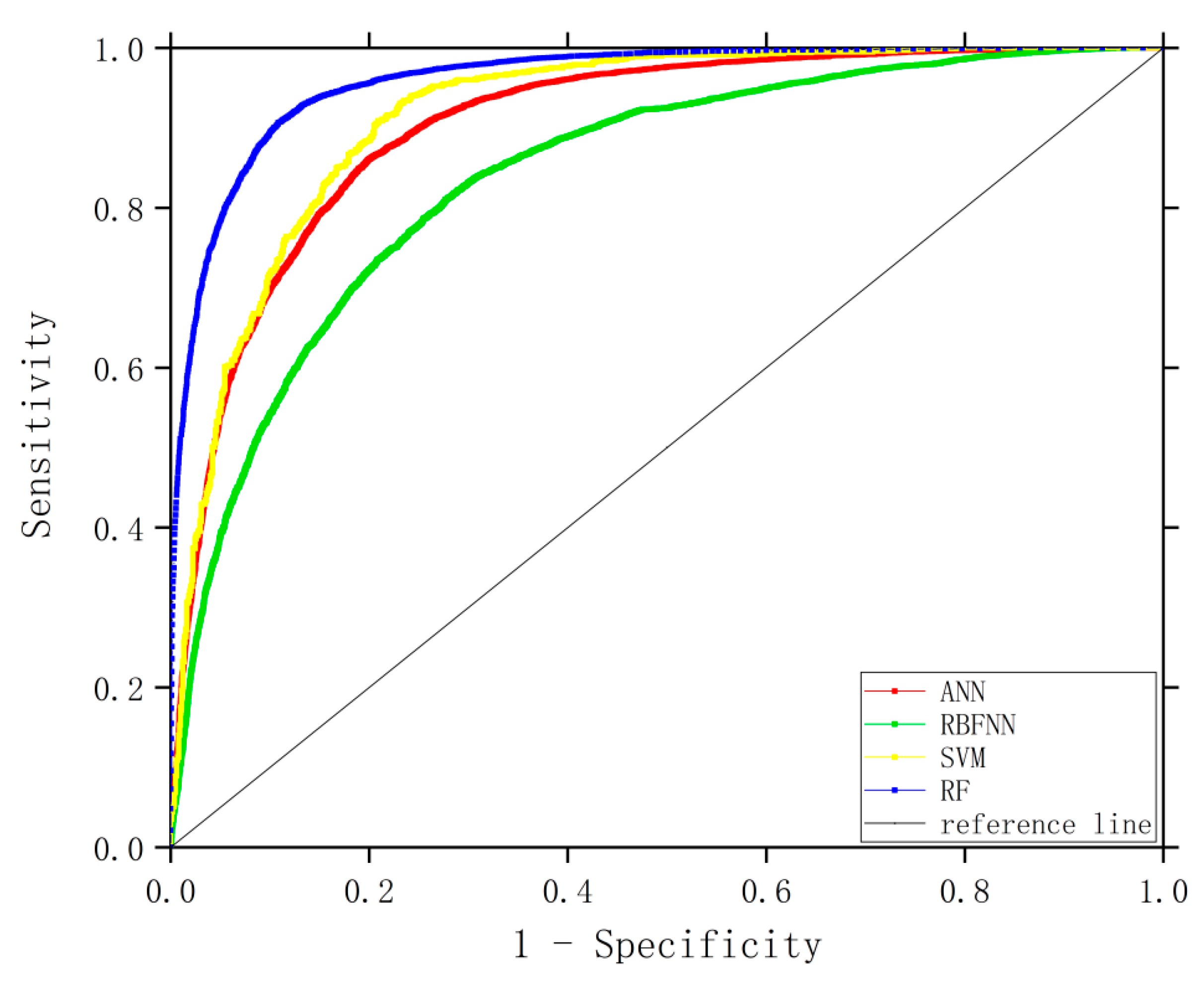
3.3. Accuracy Evaluation

We used the prediction results of the four models to construct a confusion matrix to obtain the accuracy, precision, recall, f1 value, and AUC value, as shown in

Table 6. Evaluation results of the four models.

Model	Accuracy (%)	Precision (%)	Recall (%)	f1 Value (%)	AUC
ANN	83.0	85.4	79.6	82.4	0.904
RBFNN	75.8	73.1	81.6	77.1	0.840
SVM	84.3	83.0	86.8	84.8	0.917
RF	89.2	90.2	87.9	89.0	0.960

. Figure 9 shows the ROC curves of the four models. As shown in Table 4, each model’s accuracy and f1 values were more than 75%, and the AUC value was more than 0.80. Thus, the performance of all four models was high. Among the four models, the RF model had the highest predictive ability, with an accuracy rate of 89.2%, a f1 value of 89%, and the highest AUC value, reaching 0.960. Compared with the other three models, the prediction ability of the RBF neural network was the lowest, with an accuracy rate of 75.8% and an AUC value of 0.840. As shown in Figure 11, the RF model outperformed the other three models. We therefore considered the RF model to be the most suitable among the four models for forest fire prediction in China.

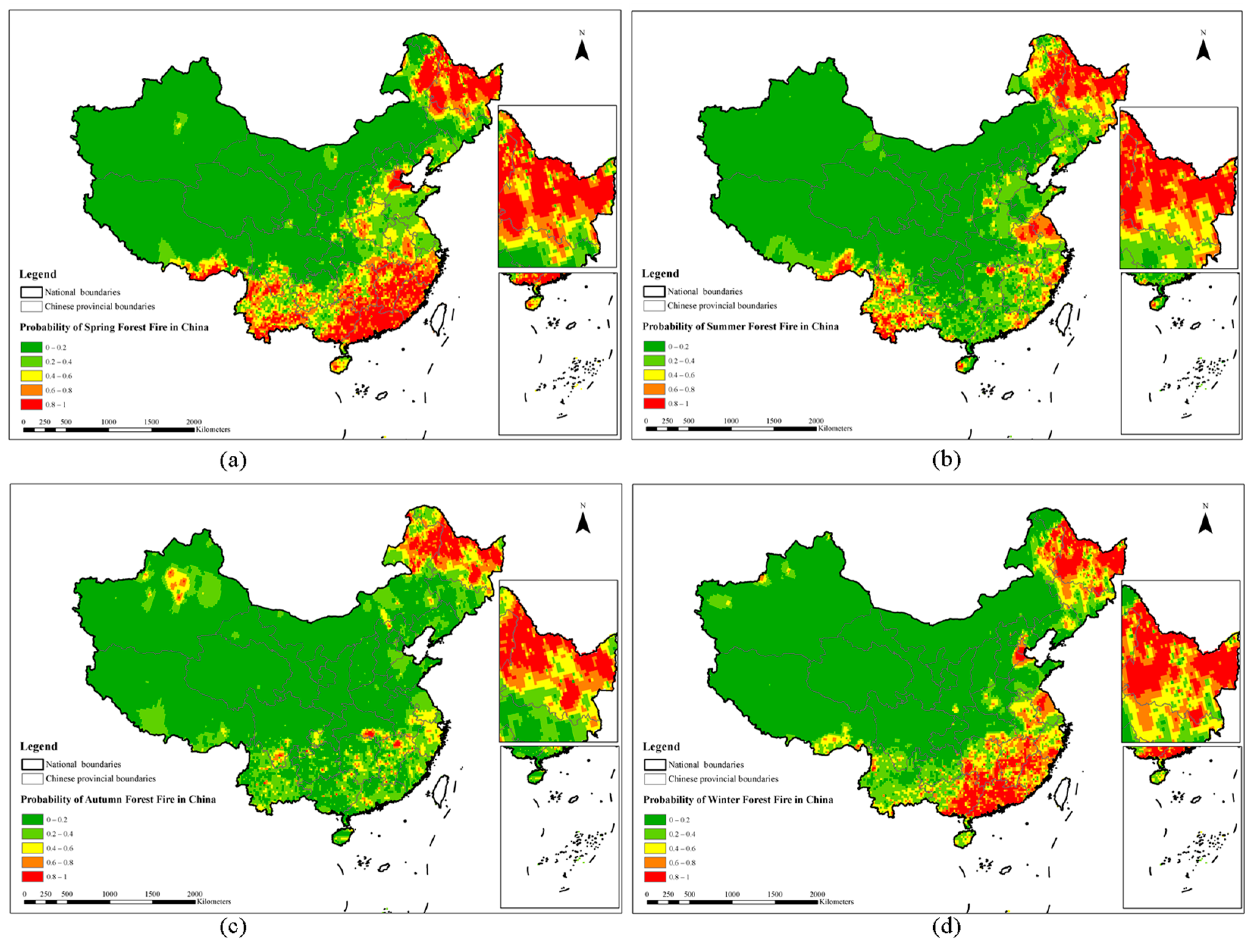
3.4. Forest Fire Risk Classification

After evaluating the accuracy of the four models, we used the RF model (highest accuracy) to obtain the probability of forest fire occurrence for the full sample. We used ArcGIS to draw a forest fire probability map (Figure 12) and a seasonal forest fire probability map (Figure 13) for China. The numbers in the legends in Figure 12 and Figure 13 indicate the predicted value of the probability of forest fires in China. For example, the likelihood of a forest fire is 1, which means that the probability of a forest fire is the greatest; the number of red areas is 0.8–1, which indicates that the area is in a high-risk state, and forest fires are very likely to occur. Figure 12 shows that the high incidence of forest fires in China is mainly concentrated in the northeast (such as the Greater Xing’an Mountains region), the southeast (such as Guangdong, Jiangxi, and Fujian), and the southwest (such as Yunnan and Sichuan). Overall, the probability of forest fires in eastern China is higher than that in western regions, and the probability of forest fires in the north and south is higher than that in Central China. Figure 13 shows that the seasonal order of the probability of forest fires in China is, from highest to lowest, spring, winter, summer, and autumn. Spring and winter are the seasons with a high incidence of forest fires, and the fires are mainly concentrated in Northeast China (such as Heilongjiang Province) and south-eastern China (such as Fujian Province and Guangdong Province).

4. Discussion

4.1. Major Forest Fire Driving Factors in China and Their Impacts

In this study, twenty factors influencing the occurrence of forest fires were selected. These factors could be divided into six categories: geographical location, meteorology, climate, topography, society, and vegetation. Researchers have studied the influencing factors of these forest fires [72,73]. The drivers of forest fires were obtained by feature selection, such as longitude, latitude, mean surface temperature, daily maximum surface temperature, cumulative precipitation, mean relative humidity, sunshine duration, mean temperature, daily maximum temperature, elevation, population, GDP, and NDVI. In terms of the importance of feature subsets, longitude and latitude had the greatest influence on the occurrence of forest fires. This result is due to the uneven distribution of forest resources and regional differences in forest resources in China. Generally, in terms of forest resources, there are more forest areas in the south than in the north, and more forest areas in the east than in the west, and there are large differences in forest types and forest classes in different regions. In addition, for example, many eucalyptus trees are planted in south-eastern provinces, such as Guangdong and Fujian, which are prone to cause fires. The planting of flammable timber forests, such as eucalyptus (driven by economic interests) has changed the forest stand structure to some extent and increased the risk of fires. Under the influence of latitude and longitude factors, the differences in forest species and forest classes in the vegetation communities of the regions are also considered.

Second, climatic factors have great impacts on forest fires, a result that is consistent with previous research results [74,75,76,77]. Temperature is one of the three necessary conditions for combustion. When the temperature reaches a certain level, forest fires are more likely to occur. The longer the duration of daylight, the higher the temperature is and the greater the likelihood of forest fires is. Rainfall and average relative humidity are other main factors affecting forest fires [53,78]; fires are likely to start when both rainfall and average relative humidity are low. In addition, altitude and vegetation can affect the occurrence of forest fires. Tian et al. (2013) believed that forest fires mainly occurred in low-altitude areas, fires are more influenced by human activities at low altitudes [79]. Chuvieco et al. (2004) found that the higher the NDVI value, the higher the vegetation cover and the more flammable trees there are, and the more likely they are to cause problems related to forest fires [80].

Forest fires are also driven by social and human factors (e.g., population and GDP). The larger the population is, the greater the human activity level in the area is, and the greater the possibility of human-caused forest fires is. Catry et al. (2007) and Sepulveda (2001) reached the same conclusion [81,82]. We believe that this difference may be due to the different data selected and the different feature selection methods. In future studies, multiple feature screening methods and analyses of different regions may be used to obtain more comprehensive results.

4.2. Optimal Choice of Forest Fire Prediction Model

We entered the forest fire driving factors selected by feature selection into the four models (ANN, RBFNN, SVM, and RF) for training. We then evaluated them using five criteria: accuracy, precision, recall rate, f1 value, and AUC value. We selected the RF model as the optimal choice for forest fire prediction. The accuracies of all four models were above 75%, which meant that they were all reliable. The results show that the RF model has the best prediction effect, followed by the SVM model, ANN model, and the RBFNN model has the worst performance. The RF algorithm can run quickly and with high accuracy on large datasets with many predictor variables. In addition, RF has high accuracy, can handle high-dimensional samples without factor screening, handles heterogeneous or missing data, and has high training and prediction speed, and can effectively eliminate model overfitting. The ANN and RBFNN models can be trained very quickly, and they can handle samples with a large amount of data, but their accuracy in this experiment is relatively low.The SVM model has a high predictive ability, but it also has certain shortcomings. The higher the model complexity, the lower the calculation speed. It takes a longer time in this model to obtain the optimal parameters when processing large amounts of sample data.

Samaher et al. (2018) used a cascade correlation network, multilayer perceptron neural network, polynomial neural network, RBF, and SVM for forest fire prediction [26]. They found that the prediction performance of the SVM was the highest, and the performance of RBFNN was the lowest, which was consistent with our conclusion. Sakr et al. (2011) used an SVM and an ANN to predict fire risk in Lebanon [41]. Their results showed that the performance of the SVM model was higher than that of the ANN model. This finding was similar to ours. Bisquert et al. (2012) used an ANN to establish a forest fire hazard model with the highest accuracy rate of 76%, which was lower than the accuracy of our model (83%) [83]. Hong (2018) used an SVM algorithm to analyse Dayu County in southwestern Jiangxi Province, China [84]. The results showed that the AUC value of the SVM was 0.75, which was lower than the value in our model (0.92). Pourtaghid et al. (2016) used an RF to conduct forest fire sensitivity analysis with a prediction accuracy of 72.8% [49]. Our model reached a prediction accuracy of 89.2%.

The four models we selected all exhibited high predictive capabilities. The main reason for this result may be that appropriate multidimensional variables have been screened out and the data sample size is large, which makes the training of each model more accurate and reliable.

4.3. Recommendations for Forest Fire Prevention

We produced a probability map for forest fires in China that showed that the highest incidences of forest fires were in the northeast (Heilongjiang Province and the northern Inner Mongolia Autonomous Region), the southeast (Fujian Province, Guangdong Province, and Jiangxi Province), and Yunnan Province. The pattern of forest fire points presented a spatial clustering distribution. Ma et al. obtained similar results [5]. For these high-incidence areas, watch towers and monitoring equipment should be added for monitoring and management. Moreover, the length of the forest fire barrier net should be increased to reduce the spread of fires. In addition, the number of fire brigades and fire vehicles should be increased to enhance the disaster-mitigation capabilities. Regarding seasonal forest fire risks, forest fire prevention and control should be emphasized in spring and winter. Strengthening fire-prevention management during these periods would mainly involve strengthening the management of human activities to reduce human-made forest fires and improving publicity and education, such as the addition of fire-prevention signs. Voice propaganda poles and signs should be set up beside forest areas or roads where people are active to remind people that it is forbidden to bring fire and flammable and explosive materials into forest areas. forest patrols during high forest fire times should be strengthened.

This study has some shortcomings, and there is room for improvement. One of the three elements of fire is combustible fuel. For the selection of forest fire driving factors, however, there is currently no way to obtain data on fuel load and other related factors. Thus, this experiment lacked relevant data such as the combustible load, particle size of combustible material, and combustible tree species. If possible, in future research, such data could be added to the forest fire prediction model.This study selected four kinds of machine learning algorithms for the forest fire prediction model. Other applicable machine learning algorithms could be used in future experiments. In addition, the ability of these machine learning algorithms to analyse spatial heterogeneity is relatively weak. Subsequent research could use geographically weighted regression to build a high-precision forest fire prediction model.

5. Conclusions

This study determined the main driving factors of forest fire occurrence in China through feature selection. The main factors affecting forest fires’ occurrence were founded as were meteorological, topographical, human and vegetation factors. Meanwhile, the differences in latitude and longitude can have a significant impact on these factors. We built four forest fire prediction models using the following machine learning algorithms: ANN, RBFNN, SVM, and RF. The results of the evaluation showed that the accuracy of all of the models was higher than 75%. Thus, these models can be used to build forest fire prediction models. Among the four models, the RF model had the highest comprehensive predictive ability, with an accuracy of 89.25%. It was therefore the optimal choice for a forest fire prediction model in China. We used the RF model to predict the probabilities of forest fires in China. Based on these probabilities, we drew a map of the probability of forest fire occurrence in China and a map of the probability of forest fires in China by season (spring, summer, autumn, and winter). Finally, based on these maps, we identified the high-incidence areas and areas at risk of forest fires. We then put forward fire prevention recommendations for the corresponding regions and seasons. This research helps to understand the main forest fire driving factors in China and provides a reference for the selection of high-precision forest fire prediction models. In future research, we will attempt to integrate geographically weighted regression with RF. This integration was expected to overcome the need to establish predefined areas to analyze forest fire drivers to address these limitations.

References

1. Venkatesh, K.; Preethi, K.; Ramesh, H. Evaluating the effects of forest fire on wa-ter balance using fire susceptibility maps. Ecol. Indic. 2020, 110, 105856. [Google Scholar] [CrossRef]
2. Sachdeva, S.; Bhatia, T.; Verma, A.K. GIS-based evolutionary optimized Gradient Boosted Decision Trees for forest fire susceptibility mapping. Nat. Hazards 2018, 92, 1399–1418. [Google Scholar] [CrossRef]
3. Zeng, X.; Yang, J.; Li, S. Spatial and temporal distribution patterns of forest fires in China from 2003–2018. For. Surv. Plan. 2021, 46, 53–58+168. [Google Scholar]
4. Hantson, S.; Pueyo, S.; Chuvieco, E. Global fire size distribution: From power law to log-normal. Int. J. Wildland Fire 2016, 25, 403. [Google Scholar] [CrossRef]
5. Prasad, A.M.; Iverson, L.R.; Liaw, A. Newer classification and regression tree techniques: Bagging and random forests for ecological prediction. Ecosystems 2006, 9, 181–199. [Google Scholar] [CrossRef]
6. Artés, T.; Cencerrado, A.; Cortés, A.; Margalef, T. Time aware genetic algorithm for forest fire propagation prediction: Exploiting multi-core platforms. Concurr. Comput. Pract. Exp. 2017, 29, 3837. [Google Scholar] [CrossRef] [Green Version]
7. Avilaflores, D.Y.; Pompagarcia, M.; Antonionemiga, X.; Rodrigueztrejo, D.A.; Vargasperez, E.; Santillan-Perez, J. Driving factors for forest fire occurrence in Durango State of Mexico: A geospatial perspective. Chin. Geogr. Sci. 2010, 20, 491–497. [Google Scholar] [CrossRef]
8. Ko, B.C.; Cheong, K.H.; Nam, J.Y. Fire detection based on vision sensor and support vector machines. Fire Saf. J. 2009, 44, 322–329. [Google Scholar] [CrossRef]
9. Liao, B.Q.; Wei, J.; Song, W.G.; Tan, C.C. Logistic and ZIP Regression Model for Forest Fire Data. Fire Saf. Sci. 2008, 3, 143–149. Available online: http://en.cnki.com.cn/Article_en/CJFDTOTAL-HZKX200803002.htm (accessed on 2 March 2008).
10. Bhusal, S.; Mandal, R. Forest fire occurrence, distribution and future risks in Arghakhanchi district, Nepal. J. Geogr. 2020, 2, 10–20. Available online: https://www.researchgate.net/publication/341701669 (accessed on 13 January 2021).
11. Bisquert, M.; Caselles, E.; Sanchez, J.M.; Caselles, V. Application of artificial neural networks and logistic regression to the prediction of forest fire danger in Galicia using MODIS data. Int. J. Wildland Fire 2012, 21, 1025–1029. [Google Scholar] [CrossRef]
12. Breiman, L. Random forests. Mach. Learn. 2001, 45, 15–32. [Google Scholar] [CrossRef] [Green Version]
13. Camp, A.; Oliver, C.; Hessburg, P.; Everett, R. Predicting late-successional fire refugia pre-dating European settlement in the Wenatchee Mountains. For. Ecol. Manag. 1997, 95, 63–77. [Google Scholar] [CrossRef]
14. Cardille, J.A.; Ventura, S.J.; Turner, M.G. Environmental and social factors influencing wildfires in the upper midwest, United States. Ecol. Appl. 2001, 11, 111–127. [Google Scholar] [CrossRef]
15. Catry, F.X.; Damasceno, P.; Silva, J.S.; Galante, M.; Moreira, F. Spatial Distribution Patterns of Wildfire Ignitions in Portugal. Modelação Espacial do Risco de Ignição em Portugal Continental, 8. In Proceedings of the 4th International Wildland Fire Conference, Sevilla, Spain, 13–17 May 2007; Project: Fire Ecology and Post-Fire Restoration. Available online: https://www.researchgate.net/publication/240613824_Spatial_Distribution_Patterns_of_Wildfire_Ignitions_in_Portugal (accessed on 1 January 2007).
16. Elmas, C.; Sönmez, Y. A data fusion framework with novel hybrid algorithm for multi-agent Decision Support System for Forest Fire. Expert Syst. Appl. 2011, 38, 9225–9236. [Google Scholar] [CrossRef]
17. Chan, C.W.; Paelinckx, D. Evaluation of random forest and adaboost tree-based ensemble classification and spectral band selection for ecotope mapping using airborne hyperspectral imagery. Remote Sens. Environ. 2008, 112, 2999–3011. [Google Scholar] [CrossRef]
18. Chang, Y.; Zhu, Z.L.; Bu, R.C.; Chen, H.W.; Feng, Y.T.; Li, Y.H.; Hu, Y.M.; Wang, Z.C. Predicting fire occurrence patterns with logistic regression in Heilongjiang Province, China. Landsc. Ecol. 2013, 28, 1989–2004. [Google Scholar] [CrossRef]
19. Chang, Y.; Zhu, Z.L.; Bu, R.C.; Li, Y.H.; Hu, Y.M. Environmental controls on the characteristics of mean number of forest fires and mean forest area burned (1987–2007) in China. For. Ecol. Manag. 2015, 356, 13–21. [Google Scholar] [CrossRef]
20. Chuvieco, E.; Aguadoa, I.; Yebraa, M. Development of a framework for fire risk assessment using remote sensing and geographic information system technologies. Ecol. Model. 2010, 221, 46–58. [Google Scholar] [CrossRef]
21. Cutler, D.R.; Edwards, T.C.; Beard, K.H. Random forests for classification in Ecology. Ecology 2007, 88, 2783–2792. [Google Scholar] [CrossRef] [PubMed]
22. Mandallaz, D.; Ye, R. Prediction of forest fires with Poisson models. Can. J. For. Res. 1997, 27, 1685–1694. [Google Scholar] [CrossRef]
23. Lin, J.; He, P.; Yang, L.; He, X.; Lu, S.; Liu, D. Predicting future urban waterlogging-prone areas by coupling the maximum entropy and FLUS model. Sustain. Cities Soc. 2022, 80, 103812. [Google Scholar] [CrossRef]
24. Adab, H.; Atabati, A.; Oliveira, S.; Moghaddam, G.A. Assessing fire hazard potential and its main drivers in Mazandaran province, Iran: A data-driven approach. Environ. Monit. Assess. 2018, 190, 670. [Google Scholar] [CrossRef]
25. Javidan, N.; Kavian, A.; Pourghasemi, H.R.; Conoscenti, C.; Jafarian, Z.; Rodrigo-Comino, J. Evaluation of multi-hazard map produced using MaxEnt machine learning technique. Sci. Rep. 2021, 11, 6496. [Google Scholar] [CrossRef] [PubMed]
26. Chen, D. Prediction of Forest Fire Occurrence in Daxing’an Mountains Based on Logistic Regression Model. For. Resour. Manag. 2019, 116–122. Available online: http://en.cnki.com.cn/Article_en/CJFDTotal-LYZY201901018.htm (accessed on 1 January 2019).
27. Bui, D.T.; Bui, Q.T.; Nguyen, Q.P.; Pradhan, B.; Nampak, H.; Trinh, P.T. A hybrid artificial intelligence approach using GIS-based neural-fuzzy inference system and particle swarm optimization for forest fire susceptibility modeling at a tropical area, Agric. Agric. For. Meteorol. 2017, 233, 32–44. [Google Scholar] [CrossRef]
28. Xie, D.W.; Shi, S.L. Prediction for burned area of forest fires based on SVM model. Appl. Mech. Mater. 2014, 513, 4084–4089. [Google Scholar] [CrossRef]
29. Dhall, A.; Dhasade, A.; Nalwade, A.; Velayudhan Kumar, M.R.; Kulkarni, V. A survey on systematic approaches in managing forest fires. Appl. Geogr. 2020, 121, 102266. [Google Scholar] [CrossRef]
30. Dickson, B.G.; Prather, J.W.; Xu, Y.; Hampton, H.M.; Aumack, E.N.; Sisk, T.D. Mapping the probability of large fire occurrence in northern Arizona, USA. Landsc. Ecol. 2006, 21, 747–761. [Google Scholar] [CrossRef]
31. Dimopoulou, M.; Giannikos, I. Towards an integrated framework for forest fire control. Eur. J. Oper. Res. 2004, 152, 476–486. [Google Scholar] [CrossRef]
32. Epifanio, I. Intervention in prediction measure: A new approach to assessing variable importance for random forests. BMC Bioinform. 2017, 18, 230. [Google Scholar] [CrossRef] [PubMed] [Green Version]
33. Erten, E.; Kurgun, V.; Musaoglu, N. Forest fire risk zone mapping from satellite imagery and GIS: A case study. In Proceedings of the XXth Congress of the International Society for Photogrammetry and Remote Sensing, Istanbul, Turkey, 12–23 July 2004; pp. 222–230. [Google Scholar]
34. Guo, F.T.; Hu, H.Q.; Jin, S.; Ma, H.Z.; Zhang, Y. Relationship between forest lighting fire occurrence and weather factors in Daxing’an Mountains based on negative binomial model and zero-inflated negative binomial models. Chin. J. Plant Ecol. 2010, 21, 159–164. Available online: http://en.cnki.com.cn/Article_en/CJFDTOTAL-ZWSB201005014.htm (accessed on 1 May 2010).
35. Guo, F.T.; Su, Z.W.; Wang, G.Y.; Sun, L.; Tigabu, M.; Yang, X.J.; Hu, H.Q. Understanding fire drivers and relative impacts in different Chinese forest ecosystems. Sci. Total Environ. 2017, 605, 411–425. [Google Scholar] [CrossRef]
36. Flannigan, M.D.; Krawchuk, M.A.; Groot, W.J.D.; Wotton, B.M. Implications of changing climate for global wildland fire. Int. J. Wildland Fire 2009, 18, 483–507. [Google Scholar] [CrossRef]
37. Guo, F.; Selvalakshmi, S.; Lin, F.; Wang, G.; Wang, W.; Su, Z.; Liu, A. Geospatial information on geographical and human factors improved anthropogenic fire occurrence modeling in the Chinese boreal forest. Can. J. For. Res. 2016, 46, 582–594. [Google Scholar] [CrossRef]
38. Ganteaume, A.; Camia, A.; Jappiot, M.; San-Miguel-Ayanz, J.; Long-Fournel, M.; Lampin, C. A review of the main driving factors of forest fire ignition over Europe. Environ. Manag. 2013, 51, 651–662. [Google Scholar] [CrossRef] [Green Version]
39. Govil, K.; Welch, M.L.; Ball, J.T.; Pennypacker, C.R. Preliminary results from a wildfire detection system using deep learning on remote camera images. Remote Sens. 2020, 12, 166. [Google Scholar] [CrossRef] [Green Version]
40. Gromping, U. Variable importance assessment in regression: Linear regression versus random forest. Am. Stat. 2009, 63, 308–319. [Google Scholar] [CrossRef]
41. Guo, F.; Wang, G.; Su, Z.; Liang, H.; Wang, W.; Lin, F.; Liu, A. What drives forest fire in Fujian, China? Evidence from logistic regression and random forests. Int. J. Wildland Fire 2016, 25, 505–519. [Google Scholar] [CrossRef]
42. Hong, H.; Naghibi, S.A.; Dashtpagerdi, M.M.; Pourghasemi, H.R.; Chen, W. A comparative assessment between linear and quadratic discriminant analyses (LDA-QDA) with frequency ratio and weights-of-evidence models for forest fire susceptibility mapping in China. Arab. J. Geosci. 2017, 10, 167. [Google Scholar] [CrossRef]
43. Soliman, H.; Sudan, K.; Mishra, A. A smart forest-fire early detection sensory system: Another approach of utilizing wireless sensor and neural networks. In Proceedings of the SENSORS, 2010 IEEE, Kona, HI, USA, 1–4 November 2010; pp. 1900–1904. [Google Scholar] [CrossRef]
44. Liang, H.L.; Lin, Y.R.; Yang, G.; Su, Z.; Wang, W.; Guo, F. Application of random forest algorithm on the forest fire prediction in Tahe area based on meteorological factors. Sci. Silvae Sin. 2016, 52, 89–98. [Google Scholar] [CrossRef]
45. Hong, H.; Tsangaratos, P.; Ilia, I.; Liu, J.; Zhu, A.X.; Xu, C. Applying genetic algorithms to set the optimal combination of forest fire related variables and model forest fire susceptibility based on data mining models. The case of Dayu County, China. Sci. Total Environ. 2018, 630, 1044–1056. [Google Scholar] [CrossRef] [PubMed]
46. Pourghasemi, H.; Beheshtirad, M.; Pradhan, B. A comparative assessment of prediction capabilities of modified analytical hierarchy process (M-AHP) and Mamdani fuzzy logic models using Netcad-GIS for forest fire susceptibility mapping. Geomat. Nat. Hazards Risk 2016, 7, 861–885. [Google Scholar] [CrossRef] [Green Version]
47. Zhao, J.; Zhang, Z.; Han, S.; Qu, C.; Yuan, Z.; Zhang, D. SVM based forest fire detection using static and dynamic features. Comput. Sci. Inf. Syst. 2011, 8, 821–841. [Google Scholar] [CrossRef]
48. Liu, K.Z.; Shu, L.F.; Zhao, F.J.; Zhang, Y.S.; Li, Y.Y. Research on spatial distribution of forest fire based on satellite hotspots data and forecasting model. J. For. Eng. 2017, 2, 128–133. Available online: http://en.cnki.com.cn/Article_en/CJFDTOTAL-LKKF201704021.htm (accessed on 1 April 2014).
49. Kane, V.R.; Lutz, J.A.; Alina Cansler, C.; Povak, N.A.; Churchill, D.J. Water balance and topography predict fire and forest structure patterns. Forest Ecol. Manag. 2015, 338, 1–13. [Google Scholar] [CrossRef]
50. Kanga, S.; Kumar, S.; Singh, S.K. Climate induced variation in forest fire using remote sensing and GIS in Bilaspur district of Himachal Pradesh. International J. Eng. Comput. Sci. 2017, 6, 21695–21702. [Google Scholar] [CrossRef]
51. Kubosova, K.; Brabec, K.; Jarkovsky, J.; Syrovatka, V. Selection of indicative taxa for river habitats: A case study on benthic macroinvertebrates using indicator species analysis and the random forest methods. Hydrobiologia 2010, 651, 101–114. [Google Scholar] [CrossRef]
52. Li, Z.; Huang, Y.; Li, X.; Xu, L. Wildland Fire Burned Areas Prediction Using Long Short-Term Memory Neural Network with Attention Mechanism. Fire Technol. 2020, 57, 1–23. [Google Scholar] [CrossRef]
53. Liu, Z.; Yang, J.; Chang, Y.; Weisberg, P.J.; He, H.S. Spatial patterns and drivers of fire occurrence and its future trend under climate change in a boreal forest of northeast China. Glob. Change Biol. 2012, 18, 2041–2056. [Google Scholar] [CrossRef]
54. Lu, A.F. Study on the relationship among forest fire, temperature and precipitation and its spatial-temporal variability in China. Agric. Sci. Technol. Hunan 2011, 12, 1396–1400. Available online: http://en.cnki.com.cn/Article_en/CJFDTOTAL-HNNT201109040.htm (accessed on 1 September 2011).
55. Denham, M.; Cortés, A.; Margalef, T.; Luque, E. Applying a dynamic data driven genetic algorithm to improve forest fire spread prediction. In Proceedings of the International Conference on Computational Science, Kraków, Poland, 23–25 June 2008; Springer: Berlin/Heidelberg, Germany, 2008; pp. 36–45. [Google Scholar] [CrossRef] [Green Version]
56. Ma, W.; Feng, Z.; Cheng, Z.; Chen, S.; Wang, F. Identifying Forest Fire Driving Factors and Related Impacts in China Using Random Forest Algorithm. Forests 2020, 11, 507. [Google Scholar] [CrossRef]
57. Maffei, C.; Menenti, M. Predicting forest fires burned area and rate of spread from pre-fire multispectral satellite measurements. ISPRS J. Photogramm. Remote Sens. 2019, 158, 263–278. [Google Scholar] [CrossRef]
58. Maingi, K.J.; Henry, M.C. Factors influencing wildfire occurrence and distribution in eastern Kentucky, USA. Int. J. Wildland Fire 2007, 16, 23–33. [Google Scholar] [CrossRef] [Green Version]
59. Boubeta, M.; Lombardía, M.J.; Marey-Pérez, M.F.; Morales, D. Prediction of forest fires occurrences with area-level poisson mixed models. J. Environ. Manag. 2015, 154, 151–158. [Google Scholar] [CrossRef]
60. Naderpour, M.; Rizeei, H.M.; Khakzad, N.; Pradhan, B. Forest fire induced Natech risk assessment: A survey of geospatial technologies. Reliab. Eng. Syst. Saf. 2019, 191, 106558. [Google Scholar] [CrossRef]
61. Oliveira, S.; Oehler, F.; San-Miguel-Ayanz, J.; Camia, A.; Pereira, J. Modeling spatial patterns of fire occurrence in Mediterranean Europe using multiple regression and random forest. Forest Ecol. Manag. 2012, 275, 117–129. [Google Scholar] [CrossRef]
62. Satir, O.; Berberoglu, S.; Donmez, C. Mapping regional forest fire probability using artificial neural network model in a Mediterranean forest ecosystem. Geomat. Nat. Hazards Risk 2016, 7, 1645–1658. [Google Scholar] [CrossRef] [Green Version]
63. Cortez, P.; Morais, A. New trends in artificial intelligence. In Proceedings of the 13th Portuguese Conference on Artificial Intelligence (EPIA 2007), Guimarães, Portugal, 3–7 December 2007; pp. 512–523. [Google Scholar]
64. Pew, K.L.; Larsen, C.P.S. GIS analysis of spatial and temporal patterns of human-caused wildfires in the temperate rainforest of Vancouver Island, Canada. Forest Ecol. Manag. 2001, 140, 1–18. [Google Scholar] [CrossRef]
65. Pourtaghi, Z.S.; Pourghasemi, H.R.; Aretano, R.; Semeraro, T. Investigation of general indicators influencing on forest fire and its susceptibility modeling using different data mining techniques. Ecol. Indic. 2016, 64, 72–84. [Google Scholar] [CrossRef]
66. Rodrigucs, M.; Dc la Riva, J. An insight into machines learning algorithms to model humarrcaused wildfire or currence. Environ. Model. Softw. 2014, 57, 192–201. [Google Scholar] [CrossRef]
67. Sakr, G.E.; Elhajj, I.H.; Mitri, G. Efficient forest fire occurrence prediction for developing countries using two weather parameters. Eng. Appl. Artif. Intell. 2011, 24, 888–894. [Google Scholar] [CrossRef]
68. Al-Janabia, S.; Al Shourbaji, I.; Salman, M.A. Assessing the suitability of soft computing approaches for forest fires prediction. Appl. Comput. Inform. 2018, 14, 214–224. [Google Scholar] [CrossRef]
69. Shang, C.; Wulder, M.A.; Coops, N.C.; White, J.C.; Hermosilla, T. Spatially-Explicit Prediction of Wildfire Burn Probability Using Remotely-Sensed and Ancillary Data. Can. J. Remote Sens. 2020, 46, 1–17. [Google Scholar] [CrossRef]
70. Singh, B.K.; Kumar, N.; Tiwari, P. Extreme Learning Machine Approach for Prediction of Forest Fires using Topographical and Metrological Data of Vietnam. In Proceedings of the 2019 Women Institute of Technology Conference on Electrical and Computer Engineering (WITCON ECE), Dehradun, India, 22–23 November 2019; pp. 104–112. [Google Scholar] [CrossRef]
71. Su, Z.W.; Liu, A.Q.; Guo, F.T.; Liang, H.L.; Wang, W.H. Driving factors and spatial distribution patteren of forest fire in Fujian Province. J. Nat. Disasters 2016, 25, 110–119. [Google Scholar] [CrossRef]
72. Syphard, A.D.; Radeloff, V.C.; Keuler, N.S.; Taylor, R.S.; Hawbaker, T.J.; Stewart, S.I.; Clayton, M.K. Predicting spatial patterns of fire on a southern California landscape. Int. J. Wildland Fire 2008, 17, 602–613. [Google Scholar] [CrossRef]
73. Tian, X.; Zhao, F.; Shu, L.; Wang, M. Distribution characteristics and the influence factors of forest fires in China. For. Ecol. Manag. 2013, 310, 460–467. [Google Scholar] [CrossRef]
74. Sevinca, V.; Kucukb, O.; Goltasc, M. A Bayesian network model for prediction and analysis of possible forest fire causes. For. Ecol. Manag. 2020, 457, 117723. [Google Scholar] [CrossRef]
75. Wang, X.C. 43 Cases of MATLAB Neural Network Analysis; Bei Hang University Press: Beijing, China, 2013. [Google Scholar]
76. Xu, X.L. Spatial Distribution Data Set of Quarterly Vegetation Index (NDVI) in China; Data Registration and Publishing System of Resources and Environmental Science Data Center of Chinese Academy of Sciences: Beijing, China, 2018; Available online: http://www.resdc.cn/ (accessed on 1 September 2011). [CrossRef]
77. Xu, Z.Q.; Su, X.Y.; Zhang, Y. Forest Fire Prediction Based on Support Vector Machine. Chin. Agric. Sci. Bull. 2012, 28, 126–131. Available online: http://en.cnki.com.cn/Article_en/CJFDTOTAL-ZNTB201213025.htm (accessed on 24 February 2012).
78. Ying, L.; Han, J.; Du, Y.; Shen, Z. Forest fire characteristics in China: Spatial patterns and determinants with thresholds. For. Ecol. Manag. 2018, 424, 345–354. [Google Scholar] [CrossRef]
79. You, Y.; Lu, C.; Wang, W.; Tang, C.-K. Relative CNN-RNN: Learning relative atmospheric visibility from images. IEEE Trans. Image Process. 2019, 28, 45–55. [Google Scholar] [CrossRef] [PubMed]
80. Li, Y.; Feng, Z.; Chen, S.; Zhao, Z.; Wang, F. Application of the Artificial Neural Network and Support Vector Machines in Forest Fire Prediction in the Guangxi Autonomous Region, China. Discret. Dyn. Nat. Soc. 2020, 2020, 14. [Google Scholar] [CrossRef] [Green Version]
81. Zhang, F.; Yang, X. Improving land cover classification in an urbanized coastal area by random forests: The role of variable selection. Remote Sens. Environ. 2020, 251, 112105. [Google Scholar] [CrossRef]
82. Su, Z.; Hu, H.; Wang, G.; Ma, Y.; Yang, X.; Guo, F. Using GIS and Random Forests to identify fire drivers in a forest city, Yichun, China. Geomat. Nat. Hazards Risk 2018, 9, 1207–1229. [Google Scholar] [CrossRef]
83. Feng, Z.; Liu, L. Estimation of forest biomass in Beijing (China) using multisource remote sensing and forest inventory data. Forests 2020, 11, 163. [Google Scholar] [CrossRef] [Green Version]
84. Zumbrunnen, T.; Pezzatti, G.B.; Menéndez, P.; Bugmann, H.; Bürgi, M.; Conedera, M. Weather and human impacts on forest fires: 100 years of fire history in two climatic regions of Switzerland. For. Ecol. Manag. 2011, 261, 2188–2199. [Google Scholar] [CrossRef]
Figure 1. Map of the study area.
Remotesensing 14 05546 g001
Figure 2. Flowchart of the Chinese forest fire occurrence prediction.
Remotesensing 14 05546 g002
Figure 3. Feature subset importance.
Remotesensing 14 05546 g003
Figure 4. Comparison charts of the predictive and actual values of the ANN.
Remotesensing 14 05546 g004
Figure 5. Comparison charts of the predictive and actual values of the RBFNN (part of the sample).
Remotesensing 14 05546 g005
Figure 6. SVC parameter selection result: (a) contour map (b) 3D view.
Remotesensing 14 05546 g006
Figure 7. Comparison charts of the predictive and actual values of the SVM (part of the sample).
Remotesensing 14 05546 g007
Figure 8. The number of trees and the accuracy of training and testing in cross-validation.
Remotesensing 14 05546 g008
Figure 9. Comparison charts of the predictive and actual values of the RF (part of the sample).
Remotesensing 14 05546 g009
Figure 10. Mean decrease accuracy of 13 variables.
Remotesensing 14 05546 g010
Figure 11. ROC curves of the four models.
Remotesensing 14 05546 g011
Figure 12. Forest fire probability map for China based on the RF model.
Remotesensing 14 05546 g012
Figure 13. Seasonal forest fire probability map for China based on the RF model: (a) spring (January, February, and March); (b) summer (April, May, and June); (c) autumn (July, August, and September); and (d) winter (October, November, and December).
Remotesensing 14 05546 g013