
Analysis of NO2 and O3 Total Columns from DOAS Zenith-Sky Measurements in South Italy
 ,
,  , ,
, ,  ,
,  and
and
Abstract
1. Introduction
2. Materials and Methods
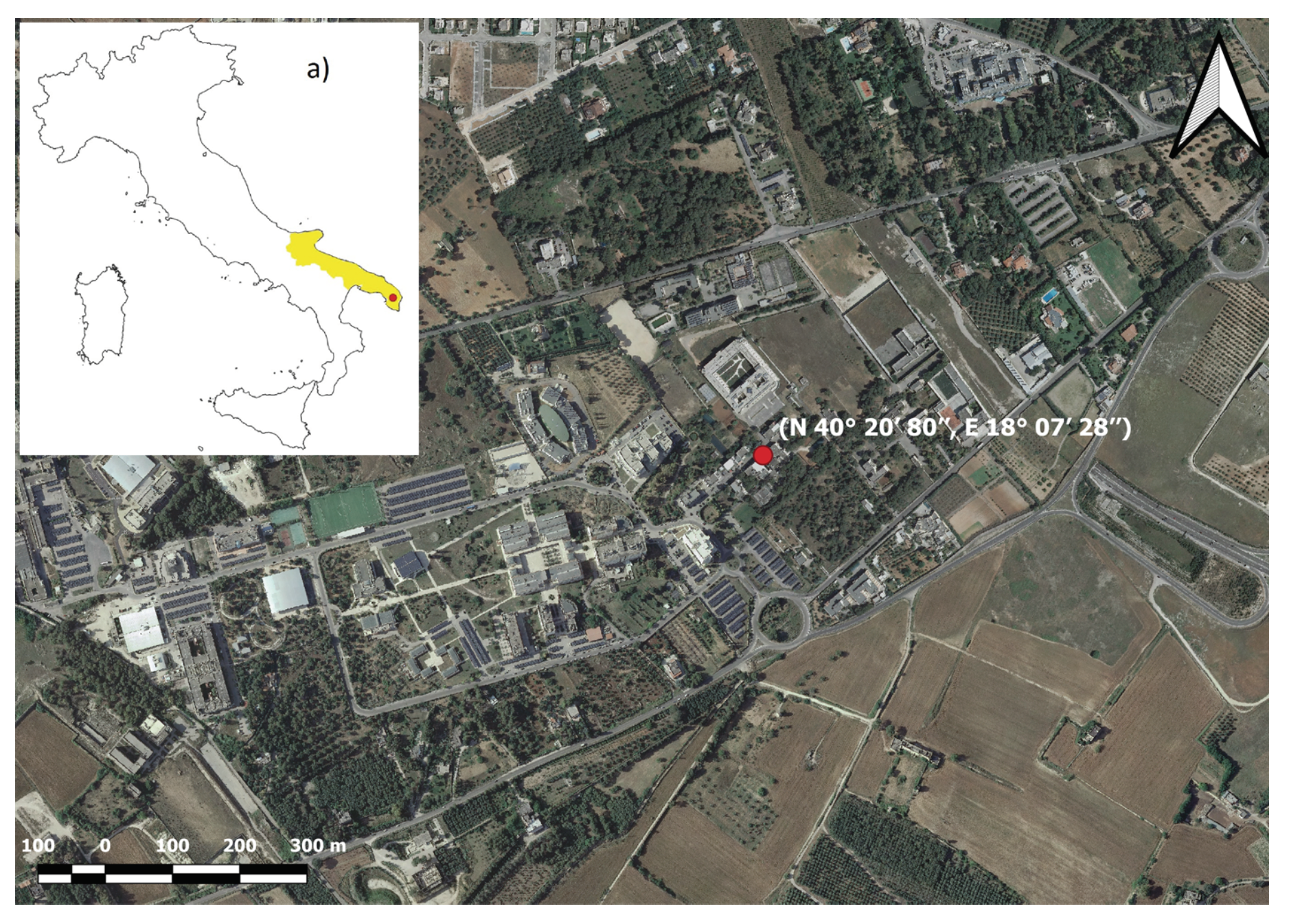
2.1. Site Description
2.2. Instruments
2.2.1. MAX-DOAS GASCOD/NG4
2.2.2. OMI
2.2.3. TROPOMI
2.3. Analysis Method
2.3.1. DOAS Methodology
2.3.2. DOAS Data Analysis: QDOAS Elaboration
- The use of daily reference spectra would have introduced daily biases in the retrieved VCDs, due to the uncertainty in the knowledge of the true contributions of the reference spectra. According to our methodology, we expected biases only between the two analysis periods.
- The two fixed reference spectra, acquired in summer at noon, are affected by a minimum gas absorption due to the almost vertical position of the sun.

| Period | beginning—28/10/2018 | 29/10/2018—end |
| Day ref. | 06/07/2017 | 11/07/2019 |
| SZA ref. | 17.62° | 18.13° |
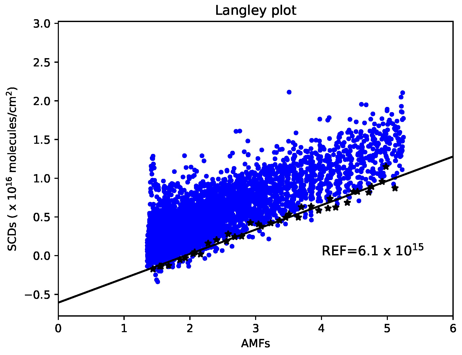
| NO2 Ref. (molec/cm) | 4.3 × 10 | 6.1 × 10 |
| O Ref. (molec/cm) | 7.1 × 10 | 1.3 × 10 |
2.3.3. Clouds and Aerosol Data Filtering
2.3.4. Reference Contributions
2.3.5. Retrieved VCDs
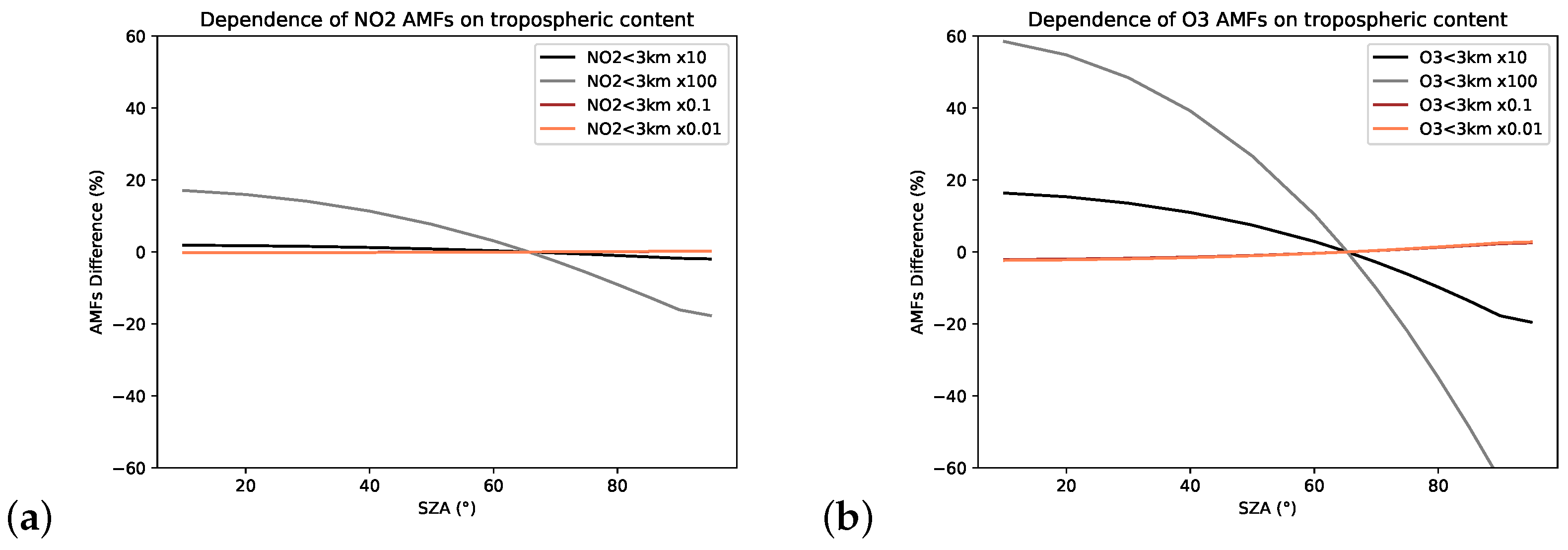
2.3.6. Systematic Errors Affecting the VCDs’ Diurnal Variability
2.3.7. Selection of Coincident Satellite Data
3. Results
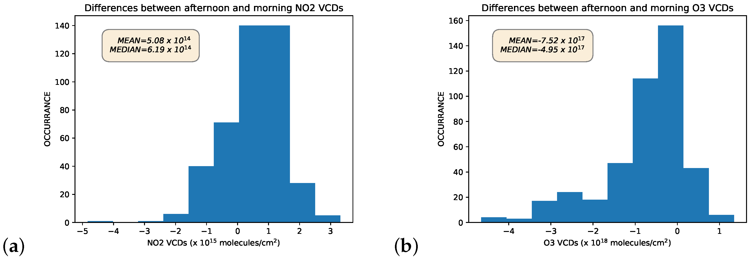
3.1. Diurnal Variability
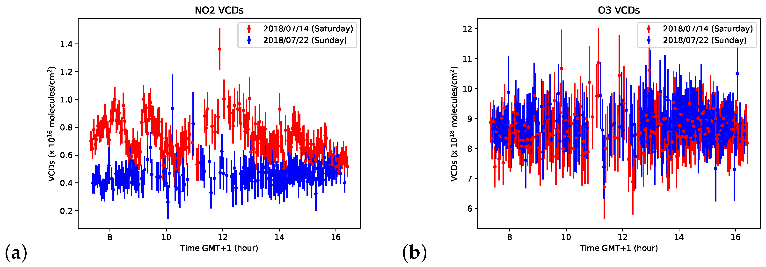
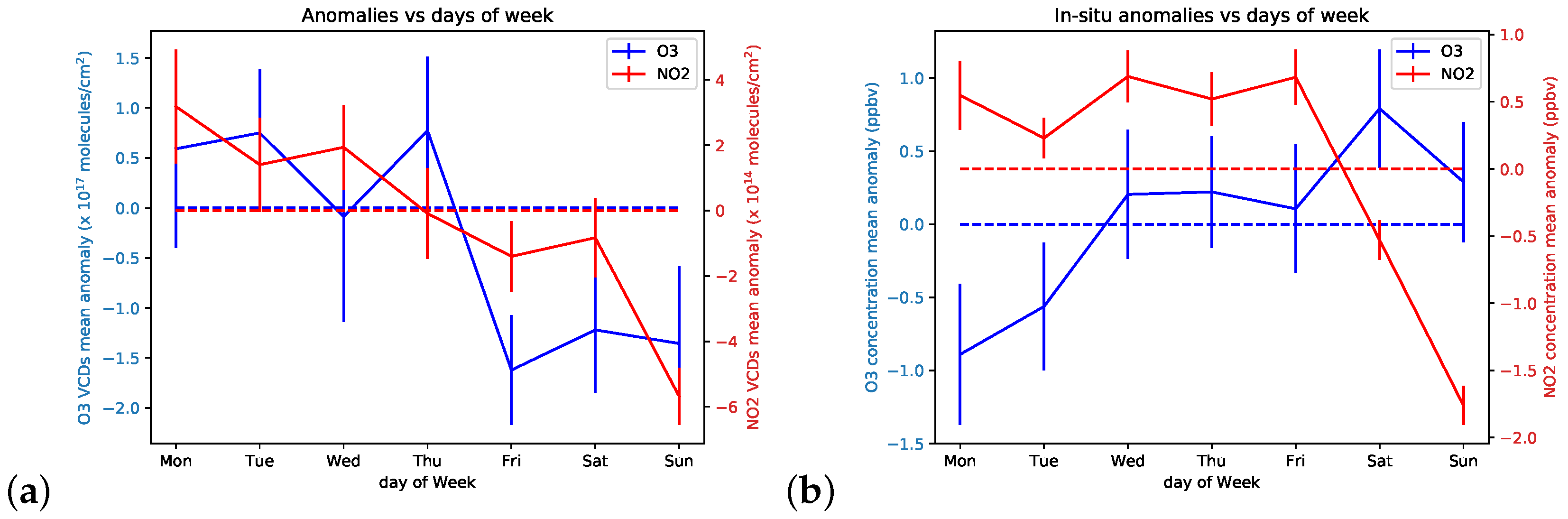
3.2. VCDs vs. Day of the Week
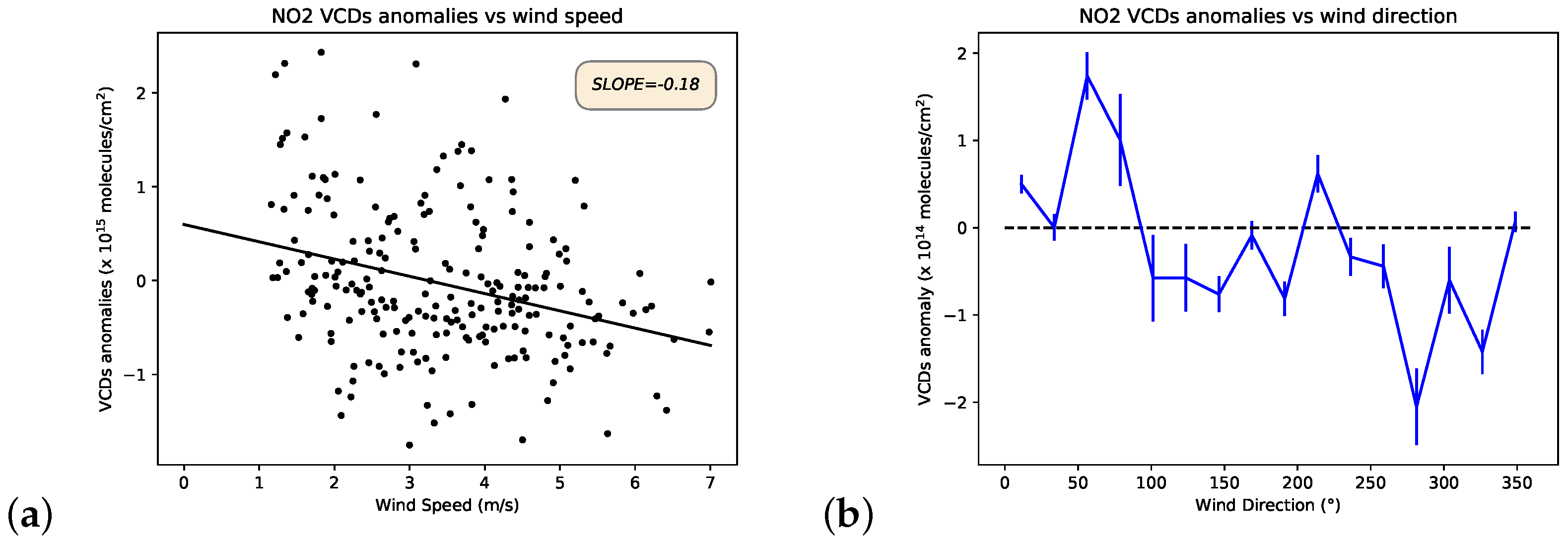
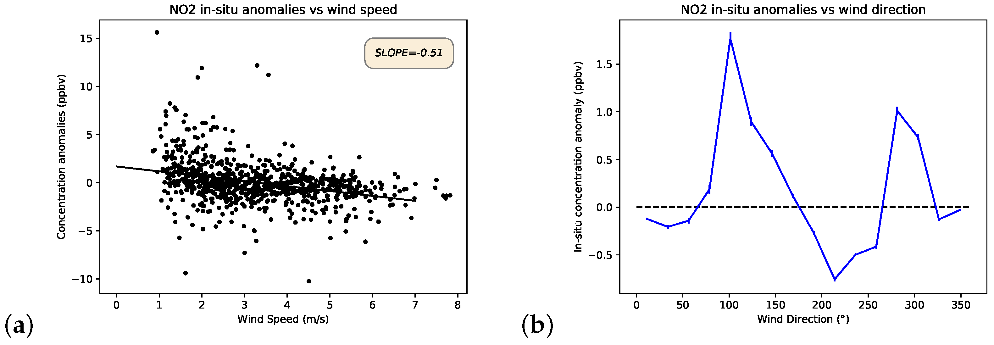
3.3. NO VCDs vs. Wind at 20 m
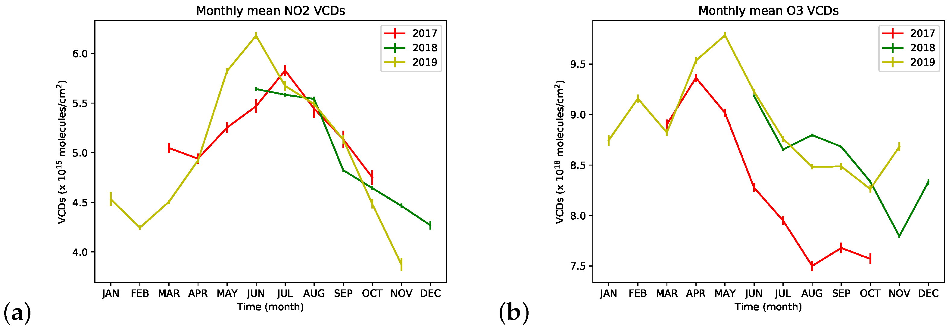
3.4. Seasonal Variability
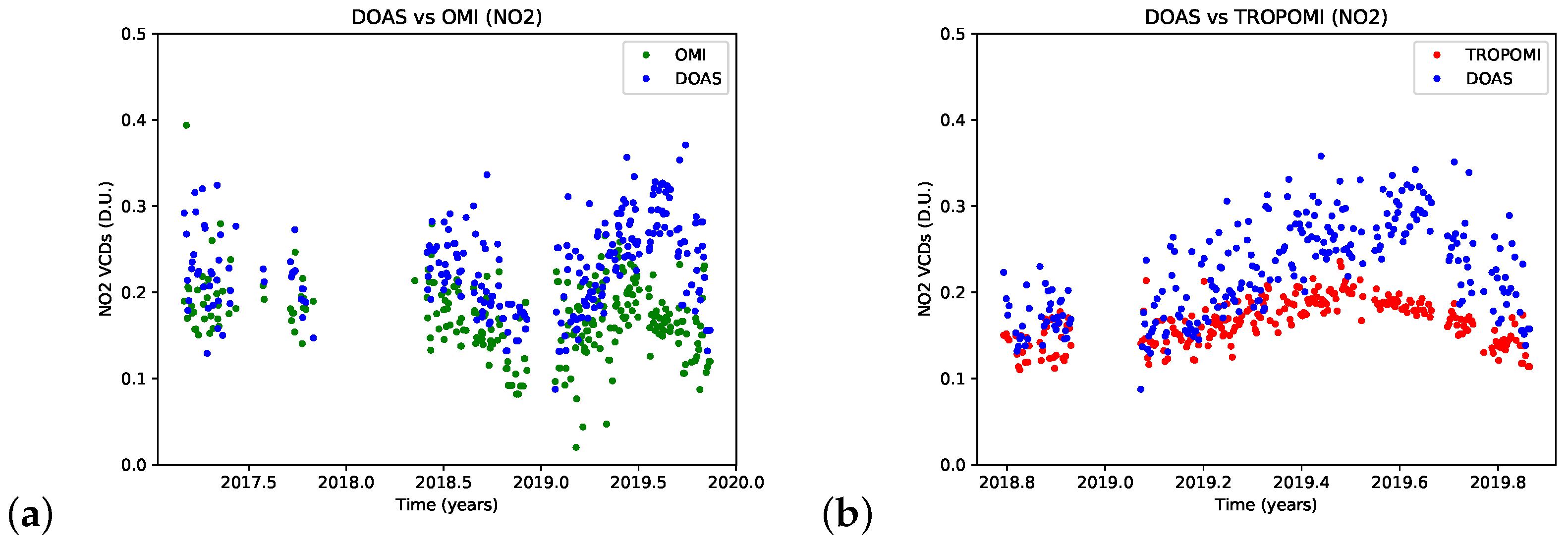
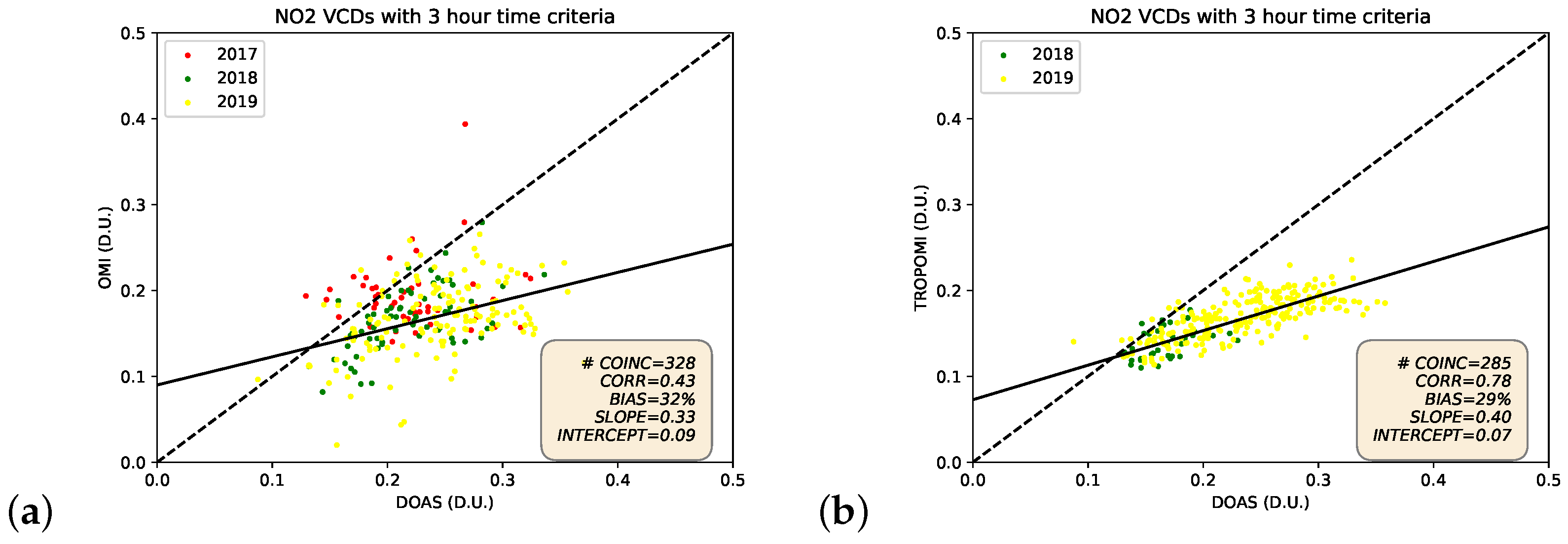
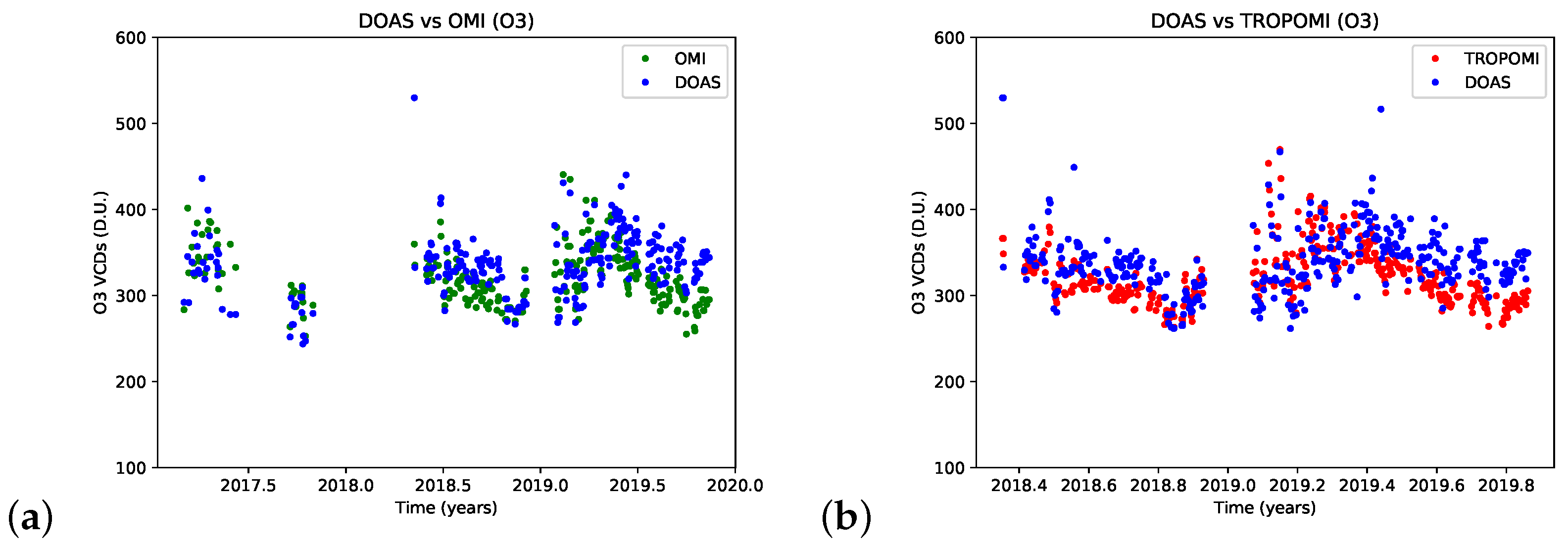
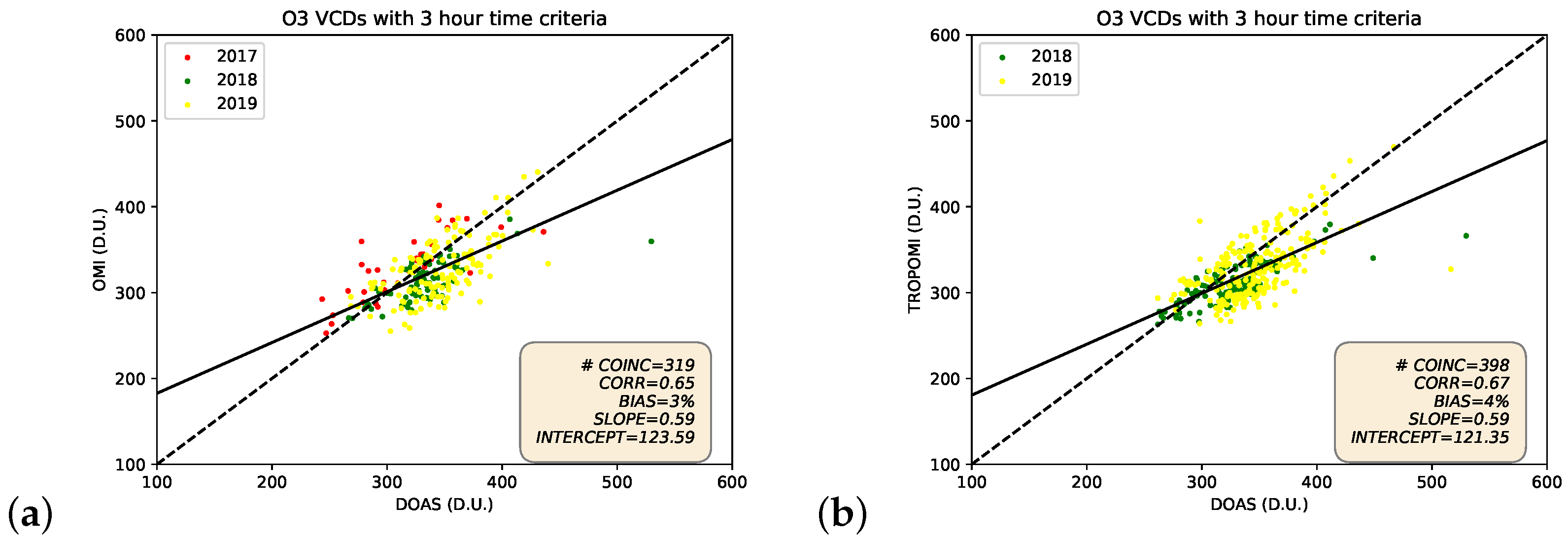
3.5. Comparison with Satellite Data
4. Discussions
5. Conclusions
Author Contributions
Funding
Institutional Review Board Statement
Informed Consent Statement
Data Availability Statement
Acknowledgments
Conflicts of Interest
References
- Pandey, S.; Kim, K.H.; Chung, S.Y.; Cho, S.J.; Kim, M.Y.; Shon, Z.H. Long-term study of NOx behavior at urban roadside and background locations in Seoul, Korea. Atmos. Environ. 2008, 42, 607–622. [Google Scholar] [CrossRef]
- Tan, P.H.; Chou, C.; Liang, J.Y.; Chou, C.C.K.; Shiu, C.J. Air pollution “holiday effect” resulting from the Chinese New Year. Atmos. Environ. 2009, 43, 2114–2124. [Google Scholar] [CrossRef]
- Jacob, D.J.; Winner, D.A. Effect of climate change on air quality. Atmos. Environ. 2009, 43, 51–63. [Google Scholar] [CrossRef]
- Chaloulakou, A.; Mavroidis, I.; Gavriil, I. Compliance with the annual NO2 air quality standard in Athens. Required NOx levels and expected health implications. Atmos. Environ. 2008, 42, 454–465. [Google Scholar] [CrossRef]
- Schwartz, J. Particulate air pollution and daily mortality in detroit. Environ. Res. 1991, 56, 204–213. [Google Scholar] [CrossRef]
- Lacis, A.A.; Wuebbles, D.J.; Logan, J.A. Radiative forcing of climate by changes in the vertical distribution of ozone. J. Geophys. Res. 1990, 95, 9971–9981. [Google Scholar] [CrossRef]
- de F. Forster, P.M.; Shine, K.P. Radiative forcing and temperature trends from stratospheric ozone changes. J. Geophys. Res. Atmos. 1997, 102, 10841–10855. [Google Scholar]
- Noxon, J.F. Tropospheric NO2. J. Geophys. Res. 1978, 83, 3051–3057. [Google Scholar] [CrossRef]
- Bond, D.W.; Zhang, R.; Tie, X.; Brasseur, G.; Huffines, G.; Orville, R.E.; Boccippio, D.J. NOx production by lightning over the continental United States. J. Geophys. Res. Atmos. 2001, 106, 27701–27710. [Google Scholar] [CrossRef]
- Zhang, R.; Tie, X.; Bond, D.W. Impacts of anthropogenic and natural NOx sources over the US on tropospheric chemistry. Proc. Natl. Acad. Sci. 2003, 100, 1505–1509. [Google Scholar] [CrossRef]
- Seinfeld, J.; Pandis, S. Atmospheric Chemistry and Physics: From Air Pollution to Climate Change; Wiley: Hoboken, NJ, USA, 2006. [Google Scholar]
- Crutzen, P.J. The influence of nitrogen oxides on the atmospheric ozone content. Q. J. R. Meteorol. Soc. 1970, 96, 320–325. [Google Scholar] [CrossRef]
- Jang, M.; Kamens, R.M. Atmospheric secondary aerosol formation by heterogeneous reactions of aldehydes in the presence of a sulfuric acid aerosol catalyst. Environ. Sci. Technol. 2001, 35, 4758–4766. [Google Scholar] [CrossRef]
- Platt, U.S.J. Differential Optical Absorption Spectroscopy; Springer: Berlin/Heidelberg, Germany, 2008. [Google Scholar]
- Hönninger, G.; von Friedeburg, C.; Platt, U. Multi axis differential optical absorption spectroscopy (MAX-DOAS). Atmos. Chem. Phys. 2004, 4, 231–254. [Google Scholar] [CrossRef]
- Frieß, U.; Monks, P.; Remedios, J.; Rozanov, A.; Sinreich, R.; Wagner, T.; Platt, U. MAX-DOAS O4 measurements: A new technique to derive information on atmospheric aerosols: 2. Modeling studies. J. Geophys. Res. Atmos. 2006, 111. [Google Scholar] [CrossRef]
- Clémer, K.; Van Roozendael, M.; Fayt, C.; Hendrick, F.; Hermans, C.; Pinardi, G.; Spurr, R.; Wang, P.; De Mazière, M. Multiple wavelength retrieval of tropospheric aerosol optical properties from MAXDOAS measurements in Beijing. Atmos. Meas. Tech. 2010, 3, 863–878. [Google Scholar] [CrossRef]
- Ma, J.; Beirle, S.; Jin, J.; Shaiganfar, R.; Yan, P.; Wagner, T. Tropospheric NO2 vertical column densities over Beijing: Results of the first three years of ground-based MAX-DOAS measurements (2008–2011) and satellite validation. Atmos. Chem. Phys. 2013, 13, 1547–1567. [Google Scholar] [CrossRef]
- Jin, J.; Ma, J.; Lin, W.; Zhao, H.; Shaiganfar, R.; Beirle, S.; Wagner, T. MAX-DOAS measurements and satellite validation of tropospheric NO2 and SO2 vertical column densities at a rural site of North China. Atmos. Environ. 2016, 133, 12–25. [Google Scholar] [CrossRef]
- Wang, S.; Cuevas, C.A.; Frieß, U.; Saiz-Lopez, A. MAX-DOAS retrieval of aerosol extinction properties in Madrid, Spain. Atmos. Meas. Tech. 2016, 9, 5089–5101. [Google Scholar] [CrossRef]
- Dimitropoulou, E.; Hendrick, F.; Pinardi, G.; Friedrich, M.M.; Merlaud, A.; Tack, F.; De Longueville, H.; Fayt, C.; Hermans, C.; Laffineur, Q.; et al. Validation of TROPOMI tropospheric NO2 columns using dual-scan multi-axis differential optical absorption spectroscopy (MAX-DOAS) measurements in Uccle, Brussels. Atmos. Meas. Tech. 2020, 13, 5165–5191. [Google Scholar] [CrossRef]
- Kang, Y.; Tang, G.; Li, Q.; Liu, B.; Cao, J.; Hu, Q.; Wang, Y. Evaluation and Evolution of MAX-DOAS-observed Vertical NO2 Profiles in Urban Beijing. Adv. Atmos. Sci. 2021, 38, 1861–9533. [Google Scholar] [CrossRef]
- Herman, J.; Abuhassan, N.; Kim, J.; Kim, J.; Dubey, M.; Raponi, M.; Tzortziou, M. Underestimation of column NO2 amounts from the OMI satellite compared to diurnally varying ground-based retrievals from multiple PANDORA spectrometer instruments. Atmos. Meas. Tech. 2019, 12, 5593–5612. [Google Scholar] [CrossRef]
- Verhoelst, T.; Compernolle, S.; Pinardi, G.; Lambert, J.C.; Eskes, H.J.; Eichmann, K.U.; Fjæraa, A.M.; Granville, J.; Niemeijer, S.; Cede, A.; et al. Ground-based validation of the Copernicus Sentinel-5p TROPOMI NO2 measurements with the NDACC ZSL-DOAS, MAX-DOAS and Pandonia global networks. Atmos. Meas. Tech. 2021, 14, 481–510. [Google Scholar] [CrossRef]
- Wang, C.; Wang, T.; Wang, P.; Rakitin, V. Comparison and Validation of TROPOMI and OMI NO2 Observations over China. Atmosphere 2020, 11, 636. [Google Scholar] [CrossRef]
- Mak, H.W.L.; Laughner, J.L.; Fung, J.C.H.; Zhu, Q.; Cohen, R.C. Improved Satellite Retrieval of Tropospheric NO2 Column Density via Updating of Air Mass Factor (AMF): Case Study of Southern China. Remote Sens. 2018, 10, 1789. [Google Scholar] [CrossRef]
- Lamsal, L.N.; Krotkov, N.A.; Vasilkov, A.; Marchenko, S.; Qin, W.; Yang, E.S.; Fasnacht, Z.; Joiner, J.; Choi, S.; Haffner, D.; et al. Ozone Monitoring Instrument (OMI) Aura nitrogen dioxide standard product version 4.0 with improved surface and cloud treatments. Atmos. Meas. Tech. 2021, 14, 455–479. [Google Scholar] [CrossRef]
- Liu, S.; Valks, P.; Pinardi, G.; Xu, J.; Chan, K.L.; Argyrouli, A.; Lutz, R.; Beirle, S.; Khorsandi, E.; Baier, F.; et al. An improved TROPOMI tropospheric NO2 research product over Europe. Atmos. Meas. Tech. 2021, 14, 7297–7327. [Google Scholar] [CrossRef]
- Donateo, A.; Conte, M.; Grasso, F.M.; Contini, D. Seasonal and diurnal behaviour of size segregated particles fluxes in a suburban area. Atmos. Environ. 2019, 219, 117052. [Google Scholar] [CrossRef]
- Donateo, A.; Feudo, T.L.; Marinoni, A.; Calidonna, C.R.; Contini, D.; Bonasoni, P. Long-term observations of aerosol optical properties at three GAW regional sites in the Central Mediterranean. Atmos. Res. 2020, 241, 104976. [Google Scholar] [CrossRef]
- Cristofanelli, P.; Busetto, M.; Calzolari, F.; Ammoscato, I.; Gullì, D.; Dinoi, A.; Calidonna, C.R.; Contini, D.; Sferlazzo, D.; Di Iorio, T.; et al. Investigation of reactive gases and methane variability in the coastal boundary layer of the central Mediterranean basin. Elem. Sci. Anthr. 2017, 5, 12. [Google Scholar] [CrossRef]
- Evangelisti, F.; Baroncelli, A.; Bonasoni, P.; Giovanelli, G.; Ravegnani, F. Differential optical absorption spectrometer for measurement of tropospheric pollutants. Appl. Opt. 1995, 34, 2737–2744. [Google Scholar] [CrossRef]
- Bortoli, D.; Silva, A.M.; Costa, M.J.; Domingues, A.F.; Giovanelli, G. Monitoring of atmospheric ozone and nitrogen dioxide over the south of Portugal by ground-based and satellite observations. Opt. Express 2009, 17, 12944–12959. [Google Scholar] [CrossRef] [PubMed]
- Bortoli, D.; Giovanelli, G.; Ravegnani, F.; Kostadinov, I.; Petritoli, A. Stratospheric nitrogen dioxide in the Antarctic. Int. J. Remote Sens. 2005, 26, 3395–3412. [Google Scholar] [CrossRef]
- Petritoli, A.; Bonasoni, P.; Giovanelli, G.; Ravegnani, F.; Kostadinov, I.; Bortoli, D.; Weiss, A.; Schaub, D.; Richter, A.; Fortezza, F. First comparison between ground-based and satellite-borne measurements of tropospheric nitrogen dioxide in the Po basin. J. Geophys. Res. Atmos. 2004, 109. [Google Scholar] [CrossRef]
- Kostadinov, I.; Petritoli, A.; Giovanelli, G.; Premuda, M.; Bortoli, D.; Masieri, S.; Ravegnani, F. Stratospheric NO2 trends over the high mountain “Ottavio Vittori” station, Italy. Int. J. Remote Sens. 2011, 32, 767–785. [Google Scholar] [CrossRef]
- Bortoli, D.; Silva, A.; Giovanelli, G. A new multipurpose UV-Vis spectrometer for air quality monitoring and climatic studies. Int. J. Remote Sens. 2010, 31, 705–725. [Google Scholar] [CrossRef]
- Levelt, P.F.; Van Den Oord, G.H.; Dobber, M.R.; Malkki, A.; Visser, H.; De Vries, J.; Stammes, P.; Lundell, J.O.; Saari, H. The ozone monitoring instrument. IEEE Trans. Geosci. Remote Sens. 2006, 44, 1093–1101. [Google Scholar] [CrossRef]
- Levelt, P.F.; Joiner, J.; Tamminen, J.; Veefkind, J.P.; Bhartia, P.K.; Stein Zweers, D.C.; Duncan, B.N.; Streets, D.G.; Eskes, H.; van der A, R.; et al. The Ozone Monitoring Instrument: Overview of 14 years in space. Atmos. Chem. Phys. 2018, 18, 5699–5745. [Google Scholar] [CrossRef]
- Krotkov, N.A.; McLinden, C.A.; Li, C.; Lamsal, L.N.; Celarier, E.A.; Marchenko, S.V.; Swartz, W.H.; Bucsela, E.J.; Joiner, J.; Duncan, B.N.; et al. Aura OMI observations of regional SO2 and NO2 pollution changes from 2005 to 2015. Atmos. Chem. Phys. 2016, 16, 4605–4629. [Google Scholar] [CrossRef]
- Bauwens, M.; Compernolle, S.; Stavrakou, T.; Müller, J.F.; van Gent, J.; Eskes, H.; Levelt, P.F.; van der A, R.; Veefkind, J.P.; Vlietinck, J.; et al. Impact of Coronavirus Outbreak on NO2 Pollution Assessed Using TROPOMI and OMI Observations. Geophys. Res. Lett. 2020, 47, e2020GL087978. [Google Scholar] [CrossRef]
- Bovensmann, H.; Burrows, J.; Buchwitz, M.; Frerick, J.; Noël, S.; Rozanov, V.; Chance, K.; Goede, A. SCIAMACHY: Mission objectives and measurement modes. J. Atmos. Sci. 1999, 56, 127–150. [Google Scholar] [CrossRef]
- Veefkind, J.; Aben, I.; McMullan, K.; Förster, H.; De Vries, J.; Otter, G.; Claas, J.; Eskes, H.; De Haan, J.; Kleipool, Q.; et al. TROPOMI on the ESA Sentinel-5 Precursor: A GMES mission for global observations of the atmospheric composition for climate, air quality and ozone layer applications. Remote Sens. Environ. 2012, 120, 70–83. [Google Scholar] [CrossRef]
- Sigrist, M.W. Air Monitoring by Spectroscopic Techniques, Chap. Differential Optical Absorption Spectroscopy (DOAS); Wiley: Hoboken, NJ, USA, 1994. [Google Scholar]
- Chance, K.V.; Spurr, R.J. Ring effect studies: Rayleigh scattering, including molecular parameters for rotational Raman scattering, and the Fraunhofer spectrum. Appl. Opt. 1997, 36, 5224–5230. [Google Scholar] [CrossRef] [PubMed]
- Aliwell, S.; Van Roozendael, M.; Johnston, P.; Richter, A.; Wagner, T.; Arlander, D.; Burrows, J.; Fish, D.; Jones, R.; Tørnkvist, K.; et al. Analysis for BrO in zenith-sky spectra: An intercomparison exercise for analysis improvement. J. Geophys. Res. Atmos. 2002, 107, ACH-10. [Google Scholar] [CrossRef]
- Vandaele, A.C.; Hermans, C.; Simon, P.C.; Carleer, M.; Colin, R.; Fally, S.; Merienne, M.F.; Jenouvrier, A.; Coquart, B. Measurements of the NO2 absorption cross-section from 42 000 cm- 1 to 10 000 cm- 1 (238–1000 nm) at 220 K and 294 K. J. Quant. Spectrosc. Radiat. Transf. 1998, 59, 171–184. [Google Scholar] [CrossRef]
- Bogumil, K.; Orphal, J.; Homann, T.; Voigt, S.; Spietz, P.; Fleischmann, O.; Vogel, A.; Hartmann, M.; Kromminga, H.; Bovensmann, H.; et al. Measurements of molecular absorption spectra with the SCIAMACHY pre-flight model: Instrument characterization and reference data for atmospheric remote-sensing in the 230–2380 nm region. J. Photochem. Photobiol. A: Chem. 2003, 157, 167–184. [Google Scholar] [CrossRef]
- Hermans, C.; Vandaele, A.C.; Carleer, M.; Fally, S.; Colin, R.; Jenouvrier, A.; Coquart, B.; Mérienne, M.F. Absorption cross-sections of atmospheric constituents: NO2, O2, and H2O. Environ. Sci. Pollut. Res. 1999, 6, 151–158. [Google Scholar] [CrossRef]
- Chance, K.; Kurucz, R.L. An improved high-resolution solar reference spectrum for earth’s atmosphere measurements in the ultraviolet, visible, and near infrared. J. Quant. Spectrosc. Radiat. Transf. 2010, 111, 1289–1295. [Google Scholar] [CrossRef]
- Wagner, T.; Dix, B.v.; Friedeburg, C.v.; Frieß, U.; Sanghavi, S.; Sinreich, R.; Platt, U. MAX-DOAS O4 measurements: A new technique to derive information on atmospheric aerosols-Principles and information content. J. Geophys. Res. Atmos. 2004, 109. [Google Scholar] [CrossRef]
- Rozanov, V.; Buchwitz, M.; Eichmann, K.U.; De Beek, R.; Burrows, J. SCIATRAN-a new radiative transfer model for geophysical applications in the 240–2400 nm spectral region: The pseudo-spherical version. Adv. Space Res. 2002, 29, 1831–1835. [Google Scholar] [CrossRef]
- Spinei, E.; Cede, A.; Herman, J.; Mount, G.; Eloranta, E.; Morley, B.; Baidar, S.; Dix, B.; Ortega, I.; Koenig, T.; et al. Ground-based direct-sun DOAS and airborne MAX-DOAS measurements of the collision-induced oxygen complex, O2O2, absorption with significant pressure and temperature differences. Atmos. Meas. Tech. 2015, 8, 793–809. [Google Scholar] [CrossRef]
- Li, K.F.; Khoury, R.; Pongetti, T.J.; Sander, S.P.; Mills, F.P.; Yung, Y.L. Diurnal variability of stratospheric column NO2 measured using direct solar and lunar spectra over Table Mountain, California (34.38°N). Atmos. Meas. Tech. 2021, 14, 7495–7510. [Google Scholar] [CrossRef]
- Pettinari, P.; Castelli, E.; Papandrea, E.; Busetto, M.; Valeri, M.; Dinelli, B.M. Towards a New MAX-DOAS Measurement Site in the Po Valley: NO2 Total VCDs. Remote Sens. 2022, 14, 3881. [Google Scholar] [CrossRef]
- Krotkov, N.A.; Lamsal, L.N.; Celarier, E.A.; Swartz, W.H.; Marchenko, S.V.; Bucsela, E.J.; Chan, K.L.; Wenig, M.; Zara, M. The version 3 OMI NO2 standard product. Atmos. Meas. Tech. 2017, 10, 3133–3149. [Google Scholar] [CrossRef]
- Van Geffen, J.; Boersma, K.F.; Eskes, H.; Sneep, M.; Ter Linden, M.; Zara, M.; Veefkind, J.P. S5P TROPOMI NO2 slant column retrieval: Method, stability, uncertainties and comparisons with OMI. Atmos. Meas. Tech. 2020, 13, 1315–1335. [Google Scholar] [CrossRef]
- Sussmann, R.; Stremme, W.; Burrows, J.; Richter, A.; Seiler, W.; Rettinger, M. Stratospheric and tropospheric NO2 variability on the diurnal and annual scale: A combined retrieval from ENVISAT/SCIAMACHY and solar FTIR at the Permanent Ground-Truthing Facility Zugspitze/Garmisch. Atmos. Chem. Phys. 2005, 5, 2657–2677. [Google Scholar] [CrossRef]
- Mavroidis, I.; Chaloulakou, A. Long-term trends of primary and secondary NO2 production in the Athens area. Variation of the NO2/NOx ratio. Atmos. Environ. 2011, 45, 6872–6879. [Google Scholar] [CrossRef]
- Chen, Y.; Wang, D.; ElAmraoui, A.; Guo, H.; Ke, X. The effectiveness of traffic and production restrictions on urban air quality: A rare opportunity for investigation. J. Air Waste Manag. Assoc. 2022; accepted. [Google Scholar] [CrossRef]
- Dirksen, R.J.; Boersma, K.F.; Eskes, H.J.; Ionov, D.V.; Bucsela, E.J.; Levelt, P.F.; Kelder, H.M. Evaluation of stratospheric NO2 retrieved from the Ozone Monitoring Instrument: Intercomparison, diurnal cycle, and trending. J. Geophys. Res. Atmos. 2011, 116. [Google Scholar] [CrossRef]
- McPeters, R.; Kroon, M.; Labow, G.; Brinksma, E.; Balis, D.; Petropavlovskikh, I.; Veefkind, J.P.; Bhartia, P.K.; Levelt, P.F. Validation of the Aura Ozone Monitoring Instrument total column ozone product. J. Geophys. Res. Atmos. 2008, 113. [Google Scholar] [CrossRef]
- Garane, K.; Koukouli, M.E.; Verhoelst, T.; Lerot, C.; Heue, K.P.; Fioletov, V.; Balis, D.; Bais, A.; Bazureau, A.; Dehn, A.; et al. TROPOMI/S5P total ozone column data: Global ground-based validation and consistency with other satellite missions. Atmos. Meas. Tech. 2019, 12, 5263–5287. [Google Scholar] [CrossRef]


| Wavelength Range | 470–510 nm |
| Polynomial | Order 3 |
| Offset | Constant |
| Cross sections | |
| NO(220 K) | from [47]. I correction (10) applied |
| NO(294 K) | from [47]. Orthogonalized to NO (220 K) with I correction (10) |
| O(223 K) | from [48]. I correction (10) applied |
| O(293 K) | from [48]. Orthogonalized to O (223 K) with I correction (10) |
| O4 (293 K) | from [49] |
| H2O (298 K) | from [49] |
| Ring | Generated according to [45], using the solar atlas in [50] |
| NO | O | |||||||||||
|---|---|---|---|---|---|---|---|---|---|---|---|---|
| OMI | TROPOMI | OMI | TROPOMI | |||||||||
| RADIUS (km) | 20 | 10 | 5 | 20 | 10 | 5 | 20 | 10 | 5 | 20 | 10 | 5 |
| COINCIDENCES | 328 | 99 | 28 | 285 | 270 | 260 | 319 | 74 | 23 | 398 | 394 | 372 |
| CORRELATION | 0.43 | 0.51 | 0.45 | 0.78 | 0.78 | 0.76 | 0.65 | 0.50 | 0.49 | 0.67 | 0.68 | 0.66 |
| BIAS (%) | 32 | 28 | 24 | 29 | 28 | 27 | 3 | 4 | 2 | 4 | 4 | 4 |
| SLOPE | 0.33 | 0.39 | 0.47 | 0.40 | 0.39 | 0.39 | 0.59 | 0.43 | 0.55 | 0.59 | 0.62 | 0.62 |
| INTERCEPT (D.U.) | 0.09 | 0.08 | 0.07 | 0.07 | 0.08 | 0.08 | 124 | 179 | 143 | 121 | 111 | 111 |
| NO | O | |||||||||||||||
|---|---|---|---|---|---|---|---|---|---|---|---|---|---|---|---|---|
| OMI | TROPOMI | OMI | TROPOMI | |||||||||||||
| SEASONS | WIN | SPR | SUM | AUT | WIN | SPR | SUM | AUT | WIN | SPR | SUM | AUT | WIN | SPR | SUM | AUT |
| COINCIDENCES | 27 | 96 | 90 | 115 | 31 | 80 | 69 | 105 | 26 | 88 | 91 | 114 | 35 | 91 | 146 | 126 |
| CORRELATION | 0.67 | 0.25 | 0.08 | 0.49 | 0.62 | 0.70 | −0.03 | 0.74 | 0.93 | 0.62 | 0.54 | 0.44 | 0.94 | 0.65 | 0.59 | 0.60 |
| BIAS (%) | 17 | 25 | 34 | 38 | 14 | 25 | 37 | 30 | −3 | −1 | 7 | 5 | −4 | 0 | 7 | 8 |
| SLOPE | 0.53 | 0.17 | 0.06 | 0.46 | 0.31 | 0.31 | −0.01 | 0.37 | 0.91 | 0.45 | 0.40 | 0.21 | 0.91 | 0.39 | 0.38 | 0.34 |
| INTERCEPT (D.U.) | 0.06 | 0.14 | 0.17 | 0.05 | 0.09 | 0.10 | 0.19 | 0.07 | 41 | 197 | 181 | 227 | 44 | 214 | 189 | 183 |
Publisher’s Note: MDPI stays neutral with regard to jurisdictional claims in published maps and institutional affiliations. |
© 2022 by the authors. Licensee MDPI, Basel, Switzerland. This article is an open access article distributed under the terms and conditions of the Creative Commons Attribution (CC BY) license (https://creativecommons.org/licenses/by/4.0/).
Share and Cite
Pettinari, P.; Donateo, A.; Papandrea, E.; Bortoli, D.; Pappaccogli, G.; Castelli, E. Analysis of NO2 and O3 Total Columns from DOAS Zenith-Sky Measurements in South Italy. Remote Sens. 2022, 14, 5541. https://doi.org/10.3390/rs14215541
Pettinari P, Donateo A, Papandrea E, Bortoli D, Pappaccogli G, Castelli E. Analysis of NO2 and O3 Total Columns from DOAS Zenith-Sky Measurements in South Italy. Remote Sensing. 2022; 14(21):5541. https://doi.org/10.3390/rs14215541
Chicago/Turabian StylePettinari, Paolo, Antonio Donateo, Enzo Papandrea, Daniele Bortoli, Gianluca Pappaccogli, and Elisa Castelli. 2022. "Analysis of NO2 and O3 Total Columns from DOAS Zenith-Sky Measurements in South Italy" Remote Sensing 14, no. 21: 5541. https://doi.org/10.3390/rs14215541
APA StylePettinari, P., Donateo, A., Papandrea, E., Bortoli, D., Pappaccogli, G., & Castelli, E. (2022). Analysis of NO2 and O3 Total Columns from DOAS Zenith-Sky Measurements in South Italy. Remote Sensing, 14(21), 5541. https://doi.org/10.3390/rs14215541