Abstract
In this era of free and open-access satellite and spatial data, modern innovations in cloud computing and machine-learning algorithms (MLAs) are transforming how Earth-observation (EO) datasets are utilized for geological mapping. This study aims to exploit the potentialities of the Google Earth Engine (GEE) cloud platform using powerful MLAs. The proposed method is implemented in three steps: (1) Based on GEE and Sentinel 2A imagery (spectral and textural features), that cover 1283 km2 area, a variety of lithological maps are generated using five supervised classifiers (random forest (RF), support vector machine (SVM), classification and regression tree (CART), minimum distance (MD), naïve Bayes (NB)); (2) the accuracy assessments for each class are performed, by estimating overall accuracy (OA) and kappa coefficient (K) for each classifier; (3) finally, the fusion of classification maps is performed using Dempster–Shafer Theory (DST) for mapping lithological units of the northern part of the complex Paleozoic massif of Rehamna, a large semi-arid region located in the SW of the western Moroccan Meseta. The results were quantitatively compared with existing geological maps, enhanced color composite and validated by field survey investigation. In comparison of individual classifiers, the SVM yields better accuracy of nearly 88%, which was 12% higher than the RF MLA; otherwise, the parametric MLAs produce the weakest lithological maps among other classifiers, with a lower OA of approximately 67%, 54% and 52% for CART, MD and NB, respectively. Noticeably, the highest OA value of 96% is achieved for the proposed approach. Therefore, we conclude that this method allows geoscientists to update previous geological maps and rapidly produce more precise lithological maps, especially for hard-to-reach regions.
1. Introduction
One of the most challenging geological applications using remote-sensing-based satellite data is mapping lithological features, especially for large and geologically complex areas that require high-precision lithological maps [1,2]. Furthermore, the limited availability of the spatial and spectral quality of open access image data (e.g., Landsat-5 TM, Landsat-7 ETM+ (enhanced thematic mapper plus), Landsat-8 OLI (operational land imager), ASTER and Sentinel-2) is widely utilized to extract lithological [3,4,5], mineral [6,7] and structural information [8,9,10]. The majority of studies investigating the potential of remote sensing for geological mapping [4,6,11,12,13] have been conducted over relatively small geographical areas using individual machine learning algorithms (MLAs). Therefore, an innovative approach, based on several factors, is implemented in this research to overcome the aforementioned issues. First, we choose well-discriminating spectral and textural information; second, we perform an efficient approach based on fused multi-classifiers to optimize accuracy; third, we exploit the high computational processing capacities of Google Earth Engine (GEE) to process free-access remote sensing (RS) geospatial big data and use MLAs over a large area.
Sentinel-2 multispectral data was used due to its high potential for geological mapping [14]. A handful of studies have investigated the potential of combining spatio-spectral bands for lithological classification over wide geologically complex regions [15,16,17]. Furthermore, different rock types with similar spectral properties can lead to spectral overlap and misclassification [18,19,20]. Hence, many classification approaches have been proposed in the literature to improve classification accuracy by introducing textural characteristics, which can be considered the most discriminating property between different lithological units when the spatial resolution of the sensor is enhanced [16,21,22].
There are several texture analysis approaches, such as the grayscale co-occurrence matrix (GLCM) [23,24], fractal analysis [25], discrete wavelet transform [26], Laplacian filter [27], Markov random field [28], granulometric analysis [29,30]. The most commonly used in geological applications is the grayscale co-occurrence matrix (GLCM) [31,32,33]. It is a second-order statistical technique that measures the relative occurrence of reference pixels compared to neighboring pixels and incorporates spatial information in the form of index images that quantify this texture. Second-order statistics have an advantage over first-order statistics since they include spatial variability information. The three principal computational parameters of GLCM are displacement, neighborhood size and quantization. According to previous researches, it is preferable to analyze the textural characteristics of high-resolution imagery with a small neighborhood size [16].
Haralick et al. [32] proposed a total of 14 second-order statistical measures that may be obtained using the GLCM probability matrix. Among them, the following four statistical metrics are frequently used: contrast, ASM, entropy and correlation [28,34]. Entropy is the most complex statistical parameter because it includes an effect related to image heterogeneity [35]. The quantification of the texture of the image facies is performed by calculating texture indices in the form of additional layers that are combined with the spectral layers in the different bands of the multispectral image. Generally, the integration of textural information within the classification algorithms enhances the lithological mapping when fewer (lower) correlated indices are used [16,22,33]. The contrast index and entropy are the lowest correlated and most discriminating indices for the texture of geological bedrock [36]. Applying these indices enhances the accuracy of classification algorithms in lithological mapping, although the amount of improvement depends on the type of rock [11]. However, the integration of spatial information in image classification approaches exposes these algorithms to a new challenge related to the processing of this multi-dimensional data (spectral, texture, geometry and shape) for large-scale geological mapping. Other issues that make lithological mapping more challenging are the limited robustness of the classification methods offered by both free and commercial software.
The application of artificial intelligence algorithms has been widely used in the field of geological applications [4,5,13]. Although many studies have attempted to compare different algorithms to determine the best classification approach for geological mapping, no consensus on the validity of the available MLAs has yet been achieved. Each classification algorithm can have very good performance for the discrimination of a lithology but may have some disadvantages when compared to other lithologies [37]. In other words, each MLA has its own pros and cons that depend on the geological complexity of the study area, the data quality of available RS imagery and the spatiospectral characteristics of each lithological unit. Therefore, the fusion approach based on multiple classifiers that merge into a single map may yield an improved result [38]. Due to its potential to increase accuracy, this technique has been gaining prospects over the last decade and is being widely used for several mapping applications, including land cover mapping [37,38,39,40], wildfire susceptibility mapping [41,42], water edge detection [43] and change detection [44], with limited application in lithological mapping. Notably, the classifier fusion method performed better when the accuracy of each classifier was more than 50%. According to theoretical and practical investigations, an optimum fusion outcome is obtained when individual classifiers are both accurate and contradictory to some classes. The Dempster–Shafer fusion (DST) [45] is one of the most frequently used fusion methods in the geospatial field; the information acquired from several sources is represented by the degree of belief/mass function, then merged/aggregated using the DST combination rule [46]. Therefore, the D-S theory is a multi-source data fusion approach for collecting more reliable data [47,48]. It is an accurate fusion technique that uses belief uncertainty intervals to provide the beliefs of hypotheses based on evidence from multiple observations [46]. The algorithm uses the reasoning, weight and probability of evidence contained in the dataset [46,47,48]. This method (DST) has been evaluated in many applications, including automatic pattern recognition [49], forensics [50] and fingerprint verification [51]. However, its application in the field of lithological mapping is non-existent [52].
The GEE (https://earthengine.google.com; Casablanca, Morocco; accessed on 5 September 2022) [53] is a free cloud computing platform that enables users to access and manage petabytes of satellite data on a large scale using JavaScript and Google’s cloud [54]. GEE uses Google’s computing capabilities to decrease uptime and provide a repository for script storage and exchange, allowing extensive user collaboration with minimal cost and equipment [55]. It provides a variety of packages for image collection, analysis, processing, classification and export to ensure that users are no longer solely dependent on expensive commercial software [55,56,57]. Several researches use GEE to take advantage of its massive data catalogue to examine dynamic processes over long time-series data and to generate large-scale thematic classifications for a variety of applications, including LU/LC mapping [58], cropland classifications [59], forest habitats mapping [60], surface water detection [61], urban and rural settlement [62], mine mapping [63], natural hazard mapping and snow and shoreline detection [64,65]. However, its application in geological mapping remains very limited [54]. This study provides an improved approach that is developed first in the GEE environment, collecting data and testing various variable combinations to enhance each classification step. Secondly, the DST fusion method was used to optimize lithological mapping and subsequently improve accuracy by considering the advantages of five MLAs classified outputs.
The novelty of this research lies in the proposed methodology for analyzing the additional value of integrating spatio-spectral bands and evaluating the performance of several MLAs available in the GEE platform for lithological classification over large geological complexes regions. Furthermore, in order to optimize and improve the classification accuracy of the exposed rock units, the fusion of multiple classifiers based on the DST method has been employed.
The study described in this paper has the following three main objectives:
- Evaluating the potential of the GEE platform and spatio-spectral bands of Sentinel-2 data to classify the lithological units exposed in a large complex semi-arid region within the GEE code editor environment;
- Evaluating and assessing the performance of different MLAs (RF, SVM, CART, MD and NB) in terms of classification accuracy of each class;
- Optimizing and enhancing lithological mapping accuracy for all the classes using the DST fusion approach.
The main goal of this research was to develop a scheme that could be adapted and deployed to produce an accurate lithological map of large geologically complex regions in a more operational and automatic approach.
2. Study Area and Materials
2.1. Study Area
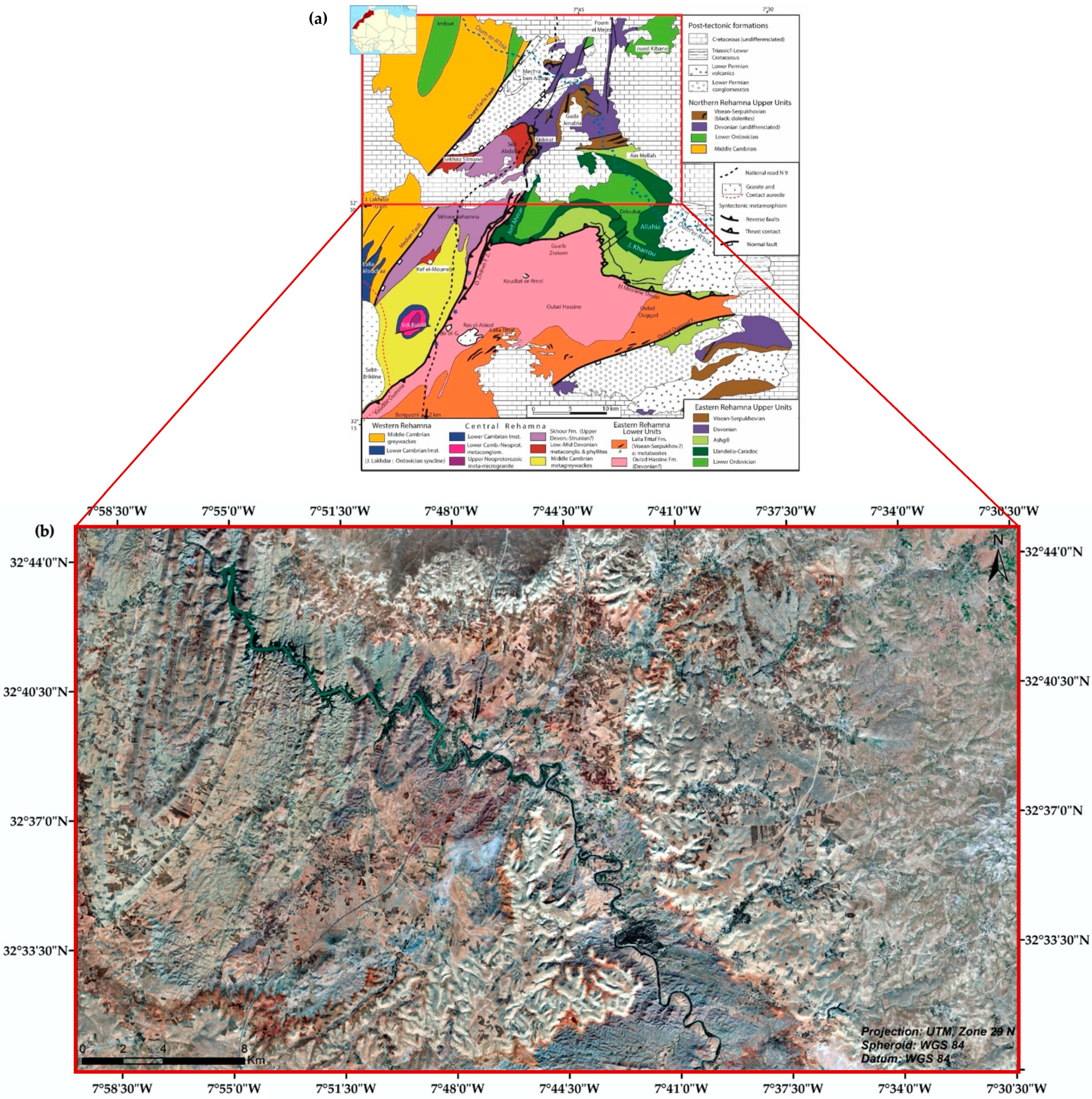
The northern part of the complex Paleozoic massif of Rehamna is chosen as a geological test site to verify the proposed approach in lithological mapping. It is characterized by good bedrock exposure because it is a dry and semi-arid region, which is situated in the SW of the western Moroccan Meseta between latitudes 32°31′N and 32°47′N and longitudes 7°31′W and 8°03′07.1″W, with a total area of approximately 1283 km2 (Figure 1). Geologically, the northern part of the Paleozoic massif of Rehamna is divided into the following two main subareas: the Paleozoic basement, which was produced during the Hercynian orogeny and eroded by preserving the paleoreliefs, and the tabular Meso-Cenozoic cover, which is slightly deformed by small normal faults [66].
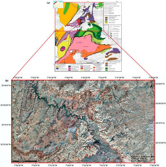
Figure 1.
(a) Location of the Paleozoic massif of Rehamna (structural and metamorphic map of the Rehamna massif); (b) Google Earth imagery of the study area with a resolution of 2 m.
The Hercynian basement formations were formed from the Cambrian to the Permian ages [66]. The Cambrian formations of the Imfout syncline are composed of siliciclastic and pyroclastic [67]. The Ordovician is also represented by coarse- to fine-grained siliciclastic terrains, particularly pelites and sandstones, with an alternation of large quartzitic bars displaying the important reliefs of Oued Kibane [67]. Clay and pelitic rocks from the Silurian are poorly exposed in the study area. The lower and middle Devonian are composed of pelites with intercalation of thin, gray bioclastic and massive limestones [68]. Otherwise, the formations of the upper Devonian are also pelitic but intercalated with quartzitic bars that are occasionally capped by a carbonate–sandstone formation that has been dated as Strunian, which is exposed in Mechra Ben Abbou and Foum el Mejez [69,70]. The Carboniferous (Upper Visean) comprises carbonate rocks and the alternation of limestone layers with pelites, in addition to pelite formation with intercalation of basic magmatic rocks, which are exposed as sills and dikes in Gada Jenabia [71]. The erosion products of the Hercynian edifice chain represent a large outcrop of the continental red deposits in the Paleozoic massif of Rehamna that comprise conglomeratic, sandstone and pelitic materials [66].
The epicontinental red cover base sediments are composed of conglomerates, sandstones and pelites. However, the underlying series comprises limestone and marl marine formations. The quaternary terraces with alluvium (conglomerate and sand) have been deposited along the Oum Er-Rbia River [66].
2.2. Data Sources and Preprocessing
In general, the preparation of the base dataset is a crucial step for any lithological classification scheme [7]. Spectral and textural features of Sentinel-2A (S2A) level-2A (L2A) optical data were used in this study. The S2A is a wide-swath, high-resolution and free-access multi-spectral instrument (MSI). It collects remote sensing datasets in 13 spectral bands situated in the visible, near infrared (VNIR), red edge (Re) and shortwave infrared (SWIR) spectral domains, with spatial resolution ranging from 10 to 60 m [72,73] (Table 1).

Table 1.
Spectral and spatial characteristics of Sentinel 2A MSI.
It is worth noting that S2A datasets used in this study were filtered by the region of interest (ROI), the period of acquisition (23 September 2020), and the highest percentage of cloud cover (10). The S2A cloud cover masking is generated using the QA60 band (60 m), which comprises dense clouds and cirrus [74]. This band is given in GEE along with the S2 surface reflectance data, as GEE reduces most of the time-consuming preprocessing steps needed in traditional computing software [54].
In the next step, satellite image spectral enhancement techniques were performed by running various methods, such as minimum noise fraction (MNF) and principal component analysis (PCA).
3. Methodology
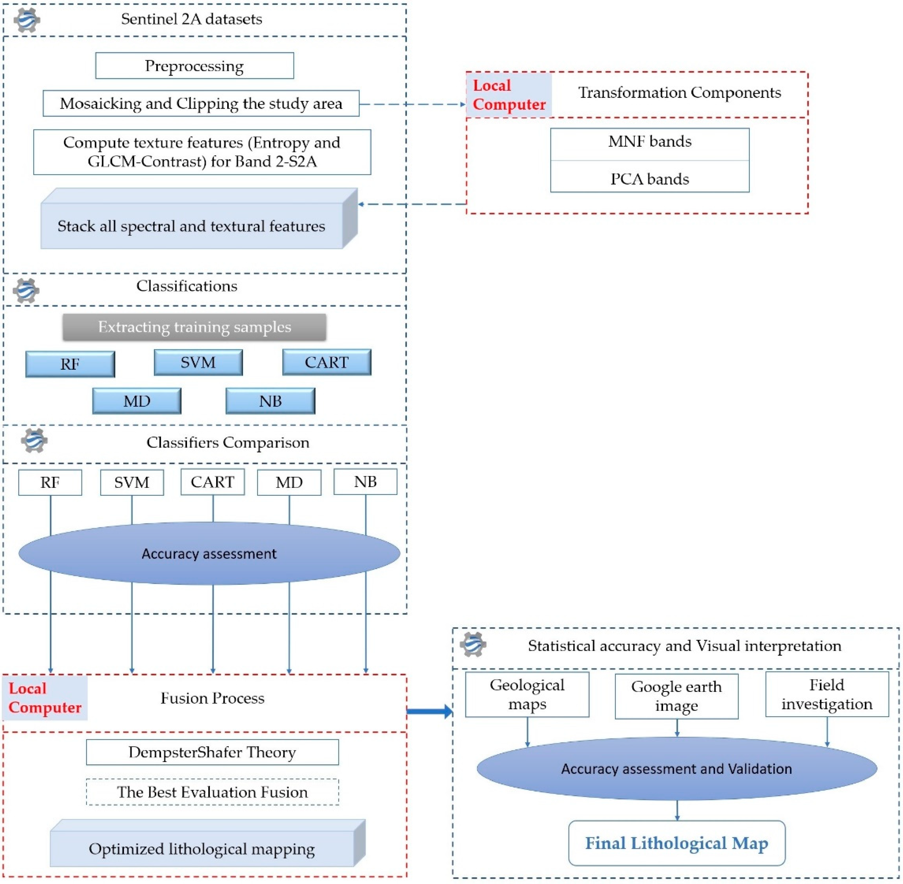
The investigation started with the integration of image spectral enhancement and spatial texture features for better discrimination of lithological units. Subsequently, a multi-classification scheme is fused for improved lithological mapping of a large, complex semi-arid area. The general processing chain of the proposed approach is displayed in Figure 2.
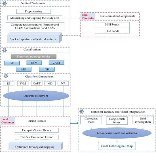
Figure 2.
Methodological workflow of the current study within GEE platform and local computer.
3.1. Data Enhancement and Processing
Various algorithms and techniques, such as principal component analysis (PCA), minimum noise fraction analysis (MNFA) and textural feature indices, were applied to Sentinel 2-A imagery in order to improve the discrimination of the lithological units exposed in the study area. The details of the processes are described below.
3.1.1. Spectral Enhancement Techniques
- Principal Component Analysis (PCA)
PCA [75] is a multivariate statistical and feature reduction process [5,76,77,78], to emphasize and highlight spectral information related to geological features by eliminating the irradiance effects of all MSI bands. It can be applied to multispectral datasets by transforming a number of correlated and high dimensional spectral bands into a set of linearly uncorrelated lower dimension output principal components (PCs) [75,79,80]. This transformation technique is performed by computing the covariance and correlation matrix and defining new orthogonal axes data, by removing redundancy in the dataset, filtering noise in the latest PCs and thereby generating enhanced contrast images represented by a false color composite (FCC) [81]. Two image components have been selected in this study (PC2 and PC5) from the application of standard PCA transformation to the VNIR and SWIR bands of S2A datasets.
- 2.
- Minimum Noise Fraction Analysis (MNFA)
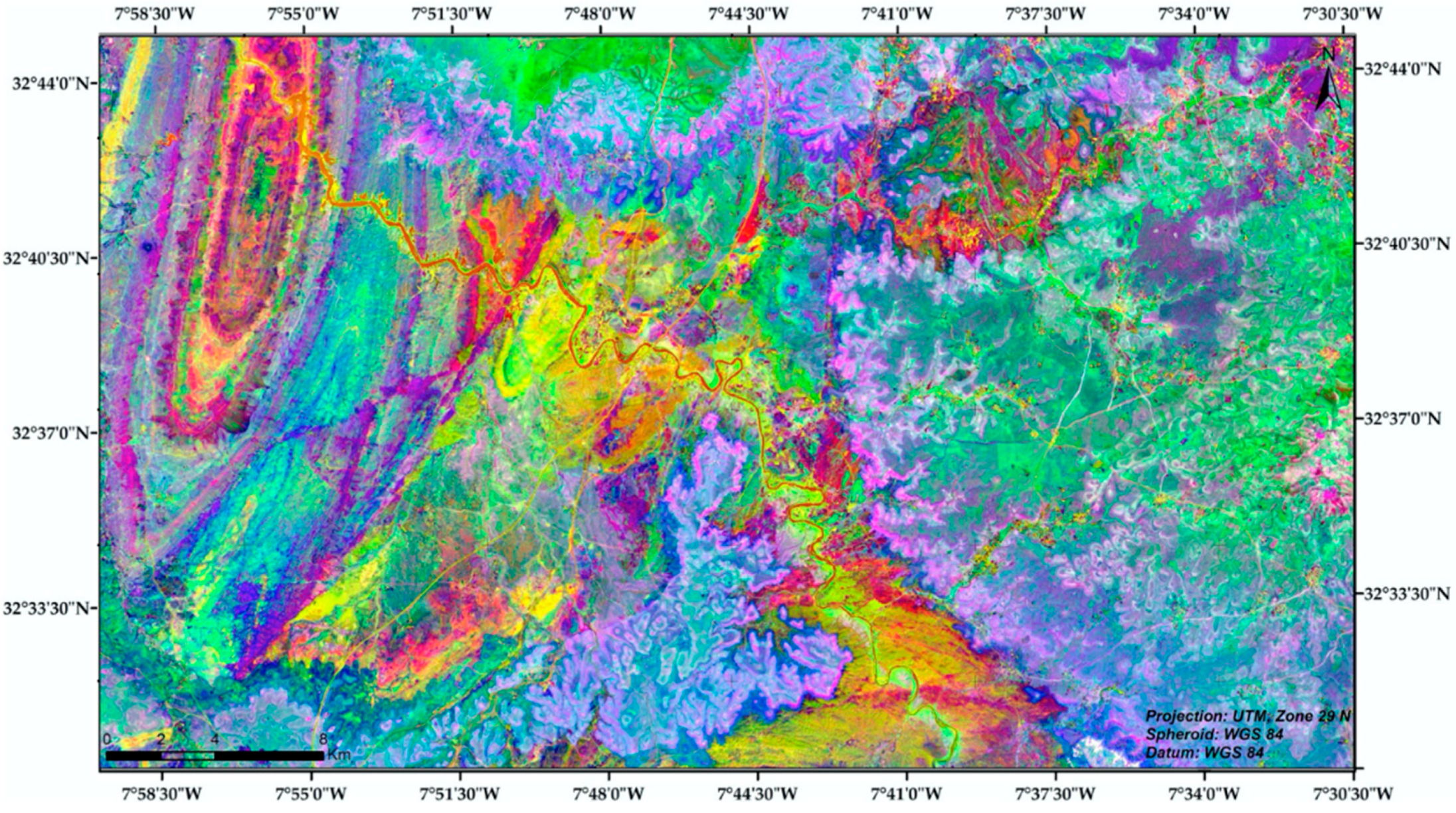
The second technique that we used is the minimum noise fraction analysis (MNFA), which is used to derive noise-free PCs, which show higher spectral contrast and showcase earth surface materials [82]. The MNF transformation involves two successive PCA rotations; the first one is also called noise-whitening and is based on the application of noise covariance matrix to decorrelate and rescale the noise in the datasets [83,84,85,86,87,88]; the second step is a standard PCA transform derived from the noise whitened data [89]. Depending on the MNFA band data, the first three components contained the largest amount of geological information and allows delineation of corresponding lithological boundaries of the study area (Figure 3).
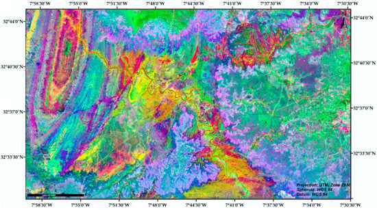
Figure 3.
The Sentinel-2A MNF bands (1, 2 and 3) combination.
3.1.2. Textural Feature Processing
The spatial features of a geological object are its shape, size and texture [21,90,91]. The latter is the simplest feature to extract from spatial datasets since it does not require a segmentation step [90]. When the texture is well quantified and exploited, it represents the spatial pattern of the gray levels of pixels and improves the discrimination of lithological units [21,90,91,92]. In geological mapping, the following several textural analysis approaches have been used: gray level co-occurrence matrix (GLCM) [23,24], fractal analysis [25], discrete wavelet transformation [26], Laplace filters [27], Markov random fields [28], granulometric analysis [29,30] or mathematical morphology analysis [93,94]. In addition to its availability on the GEE platform, the GLCM matrices are the most popular parameters for the quantification of textural information. It is a statistical computation approach of second-order histograms that uses a lot of processing techniques and produces a massive data set with many features [94]. Hence, the use of the GEE platform is preferred, which allows the extraction of GLCM matrices rapidly and easily for a large study area. Average, homogeneity, variance, entropy, contrast, dissimilarity and correlation are the texture measurements extracted from the GLCM in GEE. These parameters are frequently redundant when derived from multispectral imagery [93]. Therefore, PCA was used to select the richest image in textural information with the highest variance. In this study, only the first principal component (PC) was used to calculate the texture data since it accounts for 98.67% of total variations.
The GLCM defines a square matrix whose size Ng × Ng, with Ng is equal to the largest gray level appearing in the image. It shows that each image pixel’s spatial distribution contains textural information and is represented in Equation (1) as follows:
where the parameter d is the distance between each pair of pixels in the image, θ is the angle (generally 0°, 45°, 90° or 135°) and Ng is the number of gray levels considered in the image, n, m with n, m = 1, 2……, Ng are the gray levels of the two pixels separated by the displacement vector d of coordinates (a, b) and (x, y) are the spatial coordinates of the pixel having gray level n and (x + a, y + b) of the pixel with gray level m.
According to previous studies, it is preferable to analyze the textural properties of open access images with medium to coarse resolutions with a small moving window size [31]. Since the GLCM results depend on the values of Ng and dθ, in this study the rotation invariant was ensured by using Ng = 256, d = 1 and the average value of the GLCM obtained for 0°, 45°, 90° and 135°, with 3 × 3 moving window covering the neighboring pixels. Two texture indices, contrast (CON) and entropy (ENT), were used due to their high decorrelation as defined in Equations (2) and (3).
3.2. Machine Learning-Based Techniques
3.2.1. Random Forest (RF)
Random forest (RF), developed by Leo Breiman in 2001 [95], is a supervised non-parametric machine learning classifier that is based on bagging technique [96]. RF produces multiple trees by randomly splitting a predefined number of variables to divide at each node of the decision trees. It predicts classes using a majority vote based on the partitioning of data from numerous decision trees by implementing the Gini Index to choose the best split threshold of input variables [97,98]. This classifier requires the selection of the input variables for each decision tree (ntree) and the number of possible characteristic parameters (mtry) that can be randomly sampled for splitting at each node of the trees in the forest [95]. Therefore, among current remote sensing classification algorithms, RF has become the most extensively used in lithological mapping [5,99,100].
3.2.2. Support Vector Machine (SVM)
The support vector machine (SVM) is a popular non-parametric MLA based on the statistical learning theory proposed by Vapnik in 1995 [101]. The main aim of the SVM algorithm is to determine the optimal hyperplane (decision boundary) separating various input training samples (support vectors) from each class [102]. The parameters that need to be adjusted and optimized when using the SVM for classifying remote sensing images are the kernel function type (polynomial, sigmoid, linear and radial basis function), gamma kernel function (GKF) and the penalty parameter [103]. Studies have shown that the SVM has advantages in terms of small samples and high dimensionality [104]. However, the fast performance and accurate results make SVM one of the widely used lithological mapping classifiers [4,105].
3.2.3. Classification and Regression Tree (CART)
Classification and regression tree (CART) is a binary non-parametric decision tree classifier. It is based on a hierarchical decision tree (DT) framework, by recursively splitting parent nodes into child nodes until they reach a pre-defined threshold of non-splitable terminal nodes (also known as a “leaf node”) [106]. CART implements the information gain ratio (Gini impurity index) [107] to determine which input features will provide the optimum splitting at each node [106]. The higher Gini index value, the smaller the purity of the dataset. The great disadvantage of this technique is its extreme sensitivity to the training dataset. Even little changes in the training data can result in entirely different tree structures. However, this algorithm can create complex trees to solve complicated issues with large datasets. This classifier has been mildly used in lithological mapping [108].
3.2.4. Minimum Distance (MD)
The minimum distance (MD) classification is a classic supervised machine learning method, widely used in lithological mapping and mineral exploration [109,110,111]. It is based on computing the Euclidean distance between each image pixel vector and the mean vector for each class, in a multi-dimensional space using the mean vectors of each class [112].
3.2.5. Naïve Bayes (NB)
Naïve Bayes (NB) [113,114] is a statistical learning algorithm that uses the Bayes theorem to predict a class by estimating the highest posterior probability for each class under the naïve assumption of the inputs for each class that are conditionally independent [115]. NB has been found to be competitive against many different classification methods in a variety of practical tasks [116,117]. NB minimizes the issues of class discrimination to find class conditional marginal densities, which indicates the probability that a given sample belongs to one of the target classes [118].
3.3. Lithological Mapping Based on Dempster–Shafer Fusion
Dempster–Shafer theory (DST), also known as classical Dempster–Shafer evidence theory, is a well-defined fusion technique that uses the belief confusion matrix to combine different classified features into a new class [46]. It is a formal framework for defining and reasoning with uncertain information and which makes it possible to represent both imprecision and uncertainty using the mass function or evidence mass (m), the belief function or credibility (Cr) and the disbelief function or plausibility (pl) [119]. The masses of evidence are defined on a set called the framework of discernment Ω. This set contains the N hypotheses necessary for the complete description of the situation, as demonstrated in Equation (4) as follows [120]:
In this study, the hypotheses that describe the situation are the classes Si to which the pixels of the image are assigned as demonstrated in Equation (5) as follows:
where, N the total number of classes.
The reasoning concerns the set E of parts S of Ω given in Equation (6) as follows:
where, Card (E) = 2Ω = 2N.
The probability assignment is an evidence mass function m defined from 2N to [0, 1] that satisfies two requirements in the Equation (7) as follows:
The measure of credibility as well as that of plausibility are deduced from the mass of evidence by the following Equations (8) and (9):
with .
Where, for every S Ω, Cr(S) corresponds to the amount of information that is contained entirely within the considered subset of S by m. It contains all the knowledge crediting the veracity of this subset. pl(S) corresponds to the amount of information not discretizing S, i.e., all the information contained in the sub-assemblies having an intersection with S. These two functions are considered as the lower and higher probability [121]. Figure 4 shows graphically the relationships between Cr, Pl and uncertainty.

Figure 4.
The general DST scheme illustrates the relation between different functions.
Parallel combination of classifiers is essentially based on the errors of individual classifiers, which are usually represented in the confusion matrix for each classifier j given in Equation (10) as follows:
where, N represents the number of classes. The learning class Si is represented by row i while the class determined by classifier j is represented by column j.
The confusion matrix for each classifier is subsequently represented. When classifier j selects class , the masses of evidence will be determined by the following Equations (11) and (12):
Therefore, the recognition and the confusion probability of classifier j are defined in Equations (13) and (14) as and , respectively.
The following Equations (15) and (16) based on the classical Dempster’s rule are used to make it more flexible in terms of combining information from n classifiers represented by their mass functions mi at the same time [122,123,124]. The crucial point for merging is to add the probabilities of all the sets.
where, K is defined in Equation (17),
where, n is the number of masses of evidence or number of classifiers, N is the number of classes or hypotheses, k is the kth hypothesis, K is termed as degree of conflict in the range of [0, 1] to represent the conflict level among multiple mass of evidence, and m(S) is the orthogonal sum of n masses of evidence.
In this paper, for assigning each pixel in the fusing classifiers’ decision rules, we select the class label for which the belief function is maximal, as shown in Equation (18) as follows:
where, Sk (k = 1, 2, …, N) represents N safety levels, Sw is the result of the classification fusion of n classifiers.
The belief function is calculated by means of the Dempster–Shafer combination of Masses of Belief and indicates the belief that each input classification map presents for each label value. Moreover, the masses of belief are based on the input confusion matrices of each classification map, either by using the PRECISION or RECALL rates, or the OVERALL ACCURACY, or the KAPPA coefficient. Thus, each input classification map needs to be associated with its corresponding input confusion matrix file for the Dempster–Shafer fusion.
4. Results
In this study, Sentinel 2A imagery was used because its bands are more adequate for lithological discrimination than other satellite images due to its high spatial and spectral resolution in the VNIR to SWIR range [3]. Preprocessing, spectral subset and spatial resampling were performed on S2A remote sensing imagery using the GEE cloud platform, before attempting lithological classification using spectral and textural features. This was carried out to achieve reflectance data with bands in the same spectral range (VNIR-SWIR) and resample all image bands into a single spatial resolution (10 m). The areas covered by waterbodies, vegetation and terrace alluvium were mapped since the study area is a dry and semi-arid region. The lithological maps produced from each approach were assessed using the overall accuracy, the average accuracy of each class and the Kappa coefficient, derived from the confusion matrix. It should be noted that GEE enables us to solve the challenges concerning the data availability, data storage, data preprocessing and free computing resources, which facilitates the computationally cumbersome feature space used in this research (14 bands of spectral and textural information), in addition to the geological complexity of the study area that is characterized by multiple lithological classes (14 classes), which is time-consuming in local computing mode.
4.1. Selection of Training and Validation Samples
The selection of accurate training and validation samples is one of the most important stages in the lithological mapping process [125]. The geological maps, in situ field verification, data sources, Google Earth and enhanced color composite imagery of the study area allowed us to improve the selection of training and validation polygons. Since the classification approach employed was pixel-based, training and validation samples matched the defined lithological units to which they belonged, hence avoiding mixed pixel issues. A visual approach was used on the reference datasets to collect 480 polygons that were manually selected, with the same number of samples for each category (approximately 30 polygons for each class) distributed over the study area for all the classes in the GEE map area environment, where the reference samples were divided into two sets of 75% training and 25% validation samples.
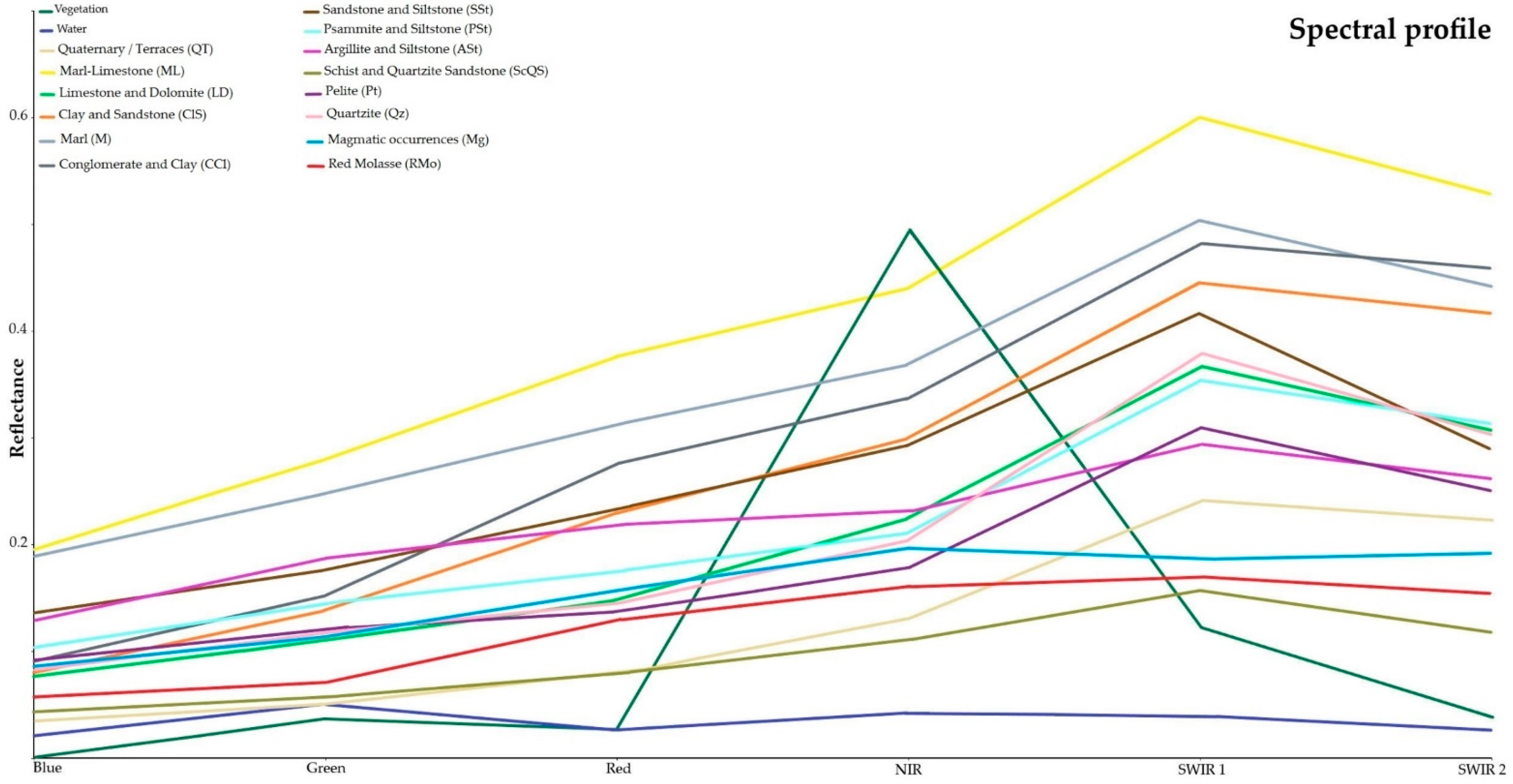
Figure 5 shows the variation of an average of all training samples derived from the study area for Sentinel 2A bands. It illustrates that vegetation and water features have different spectral properties than lithological units.
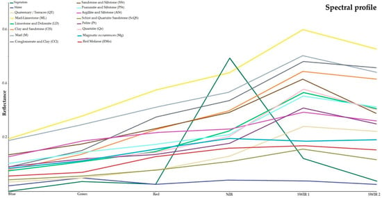
Figure 5.
Average reflectance spectra of representative bedrock outcrops based on training samples selected from Sentinel 2A.
4.2. Classification Schemes
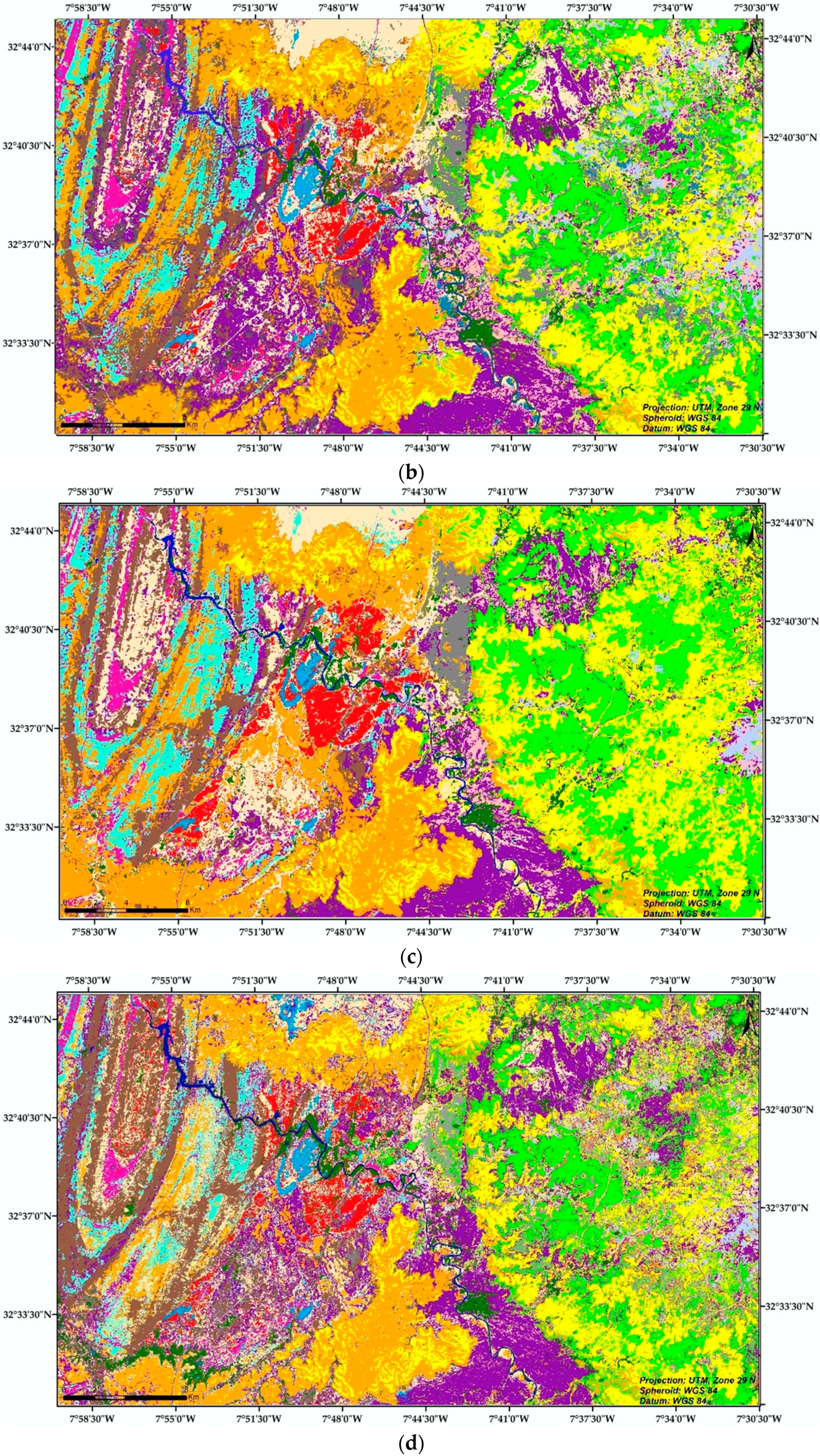
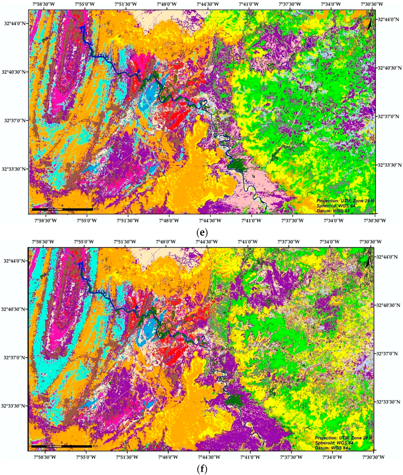
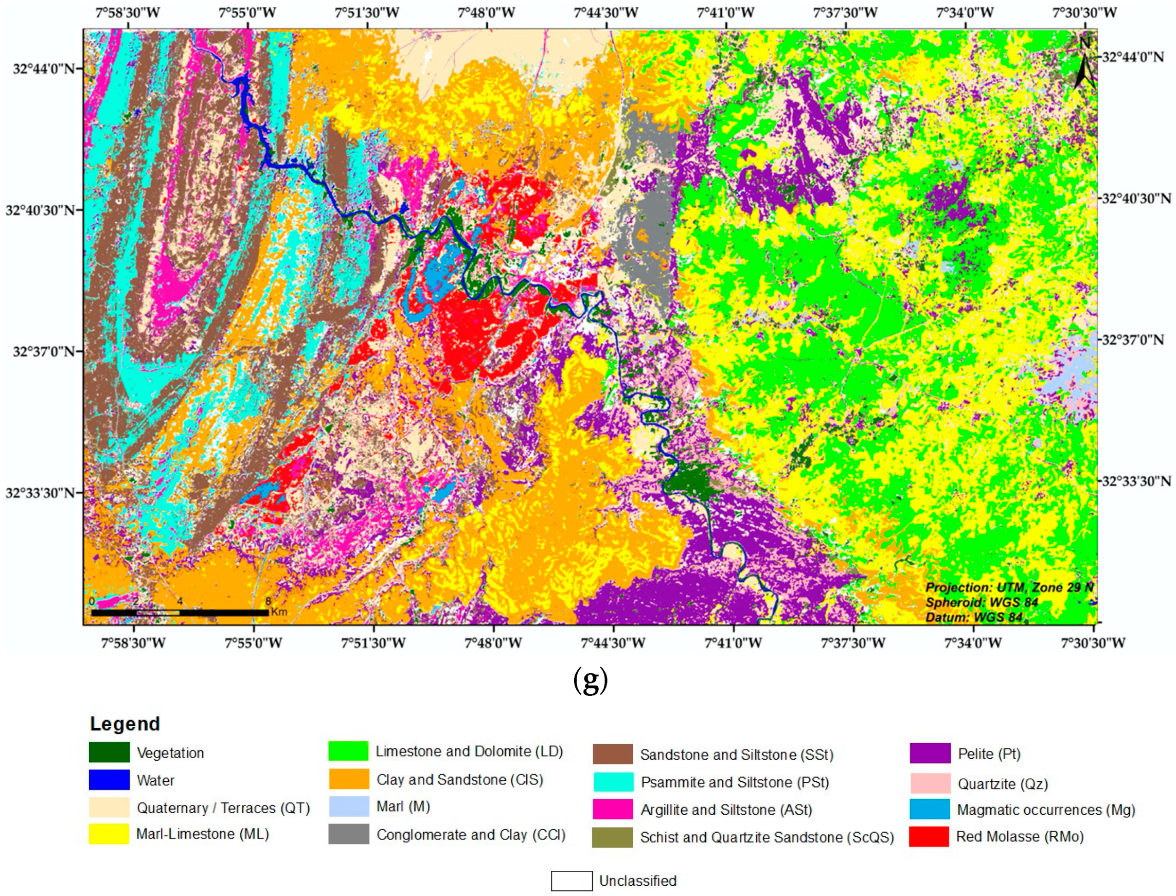
Machine learning algorithms, including RF, SVM, CART, MD and NB, were used to classify spectral and textural features of Sentinel 2A, within the GEE cloud computing platform, in the northern part of the complex Paleozoic massif of Rehamna, to identify lithological units. All models were well trained by optimal parameters. The five classification algorithms and the proposed method results for the rocky outcrops are shown in Figure 6.
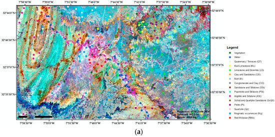
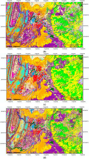
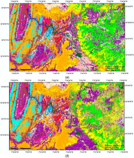
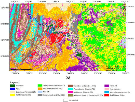
Figure 6.
(a) Location of the training samples polygons superposed on the RGB color composite generated with the PC2, MNF1 and MNF3 bands. Lithological maps of the study area by: (b) random forest (RF); (c) support vector machine (SVM); (d) classification regression tree (CART); (e) minimum distance (MD); (f) naïve Bayes (NB); (g) using the proposed approach.
The classification results obtained using parametric classifiers, particularly CART (Figure 6d), MD (Figure 6e) and NB (Figure 6f), provide more noise than other methods. However, the lithological units comprised of siltstone were well-mapped using parametric algorithms. According to the pre-existing geological maps [66], the lithological units extracted using RF (Figure 6b) and SVM (Figure 6c), non-parametric MLAs, are more precise in detecting bedrock units (pelites, quartzite) and sedimentary rocks (limestone, sandstone, dolomite), respectively. However, the proposed fusion method using DST had high consistency in terms of all rock types exposed in the study area, as shown in Figure 6g.
4.3. Accuracy Assessments of Classified Maps
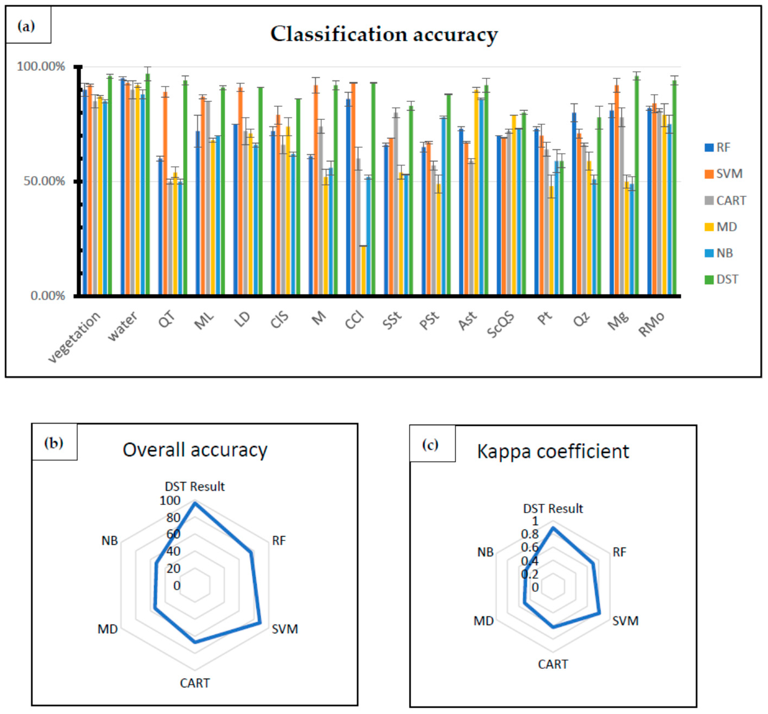
The accuracy estimates of the lithological mapping results of the ML classifiers available in GEE and the proposed method based on DST are displayed in Figure 7. Among the results obtained using different MLAs, it can be observed that the average value of OAs of non-parametric classifiers, particularly SVM and RF, were higher than those of parametric MLAs, namely, CART, MD and NB. Otherwise, the proposed approach, based on DST, effectively maximizes the classification accuracy by registering values of and for OA and K coefficient, respectively, which indicates that this method is more accurate in recognizing and classifying the lithological units in remote sensing images.
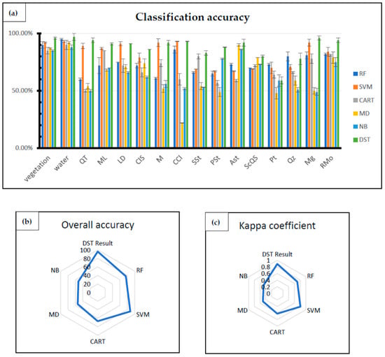
Figure 7.
(a) The average classification accuracies standard deviation of each class; (b) overall accuracies; (c) Kappa coefficient using several machine learning algorithms and DST result.
5. Discussion
Unlike the majority of previous studies that adopted individual MLAs using third-party software for lithological mapping of small geographical areas [3,4,13,126,127,128,129], we exploit the capabilities of the GEE cloud computing platform to perform the MLAs procedure using the spatio-spectral data from Sentinel 2. The spatial information was used as a pixel local variability in band measurements (entropy and contrast) contained in the texture index images extracted from the GLCMs. Then, we transferred it to a local computer to train the DST fusion technique by integrating all the MLAs results to produce an optimized lithological map. This is a point of novelty in our study.
The use of the GEE environment offers a variety of open-access geospatial big data and various algorithms (preprocessed spatial models and classifiers), which allow us to create and manage multiple workflows, in order to produce detailed large-scale maps in a cost- and time-efficient manner relative to traditional computing software [54,56]. In this platform, we used five supervised machine learning classification algorithms (RF, SVM, CART, MD, NB) to construct a lithological map in the northern part of the complex Paleozoic massif of Rehamna, based on the spatio-spectral characteristics of Sentinel 2A without needing to purchase or download any software or datasets.
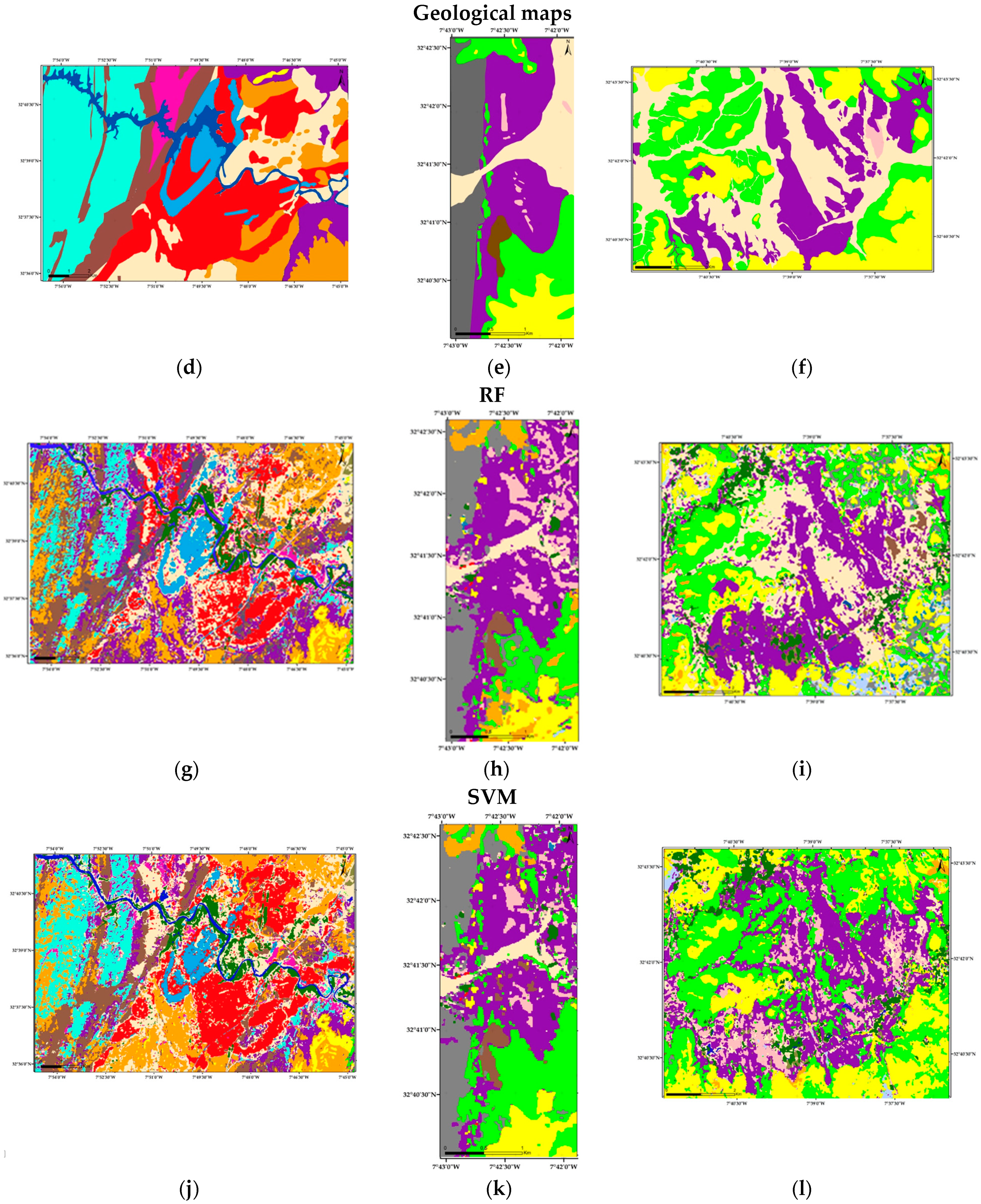
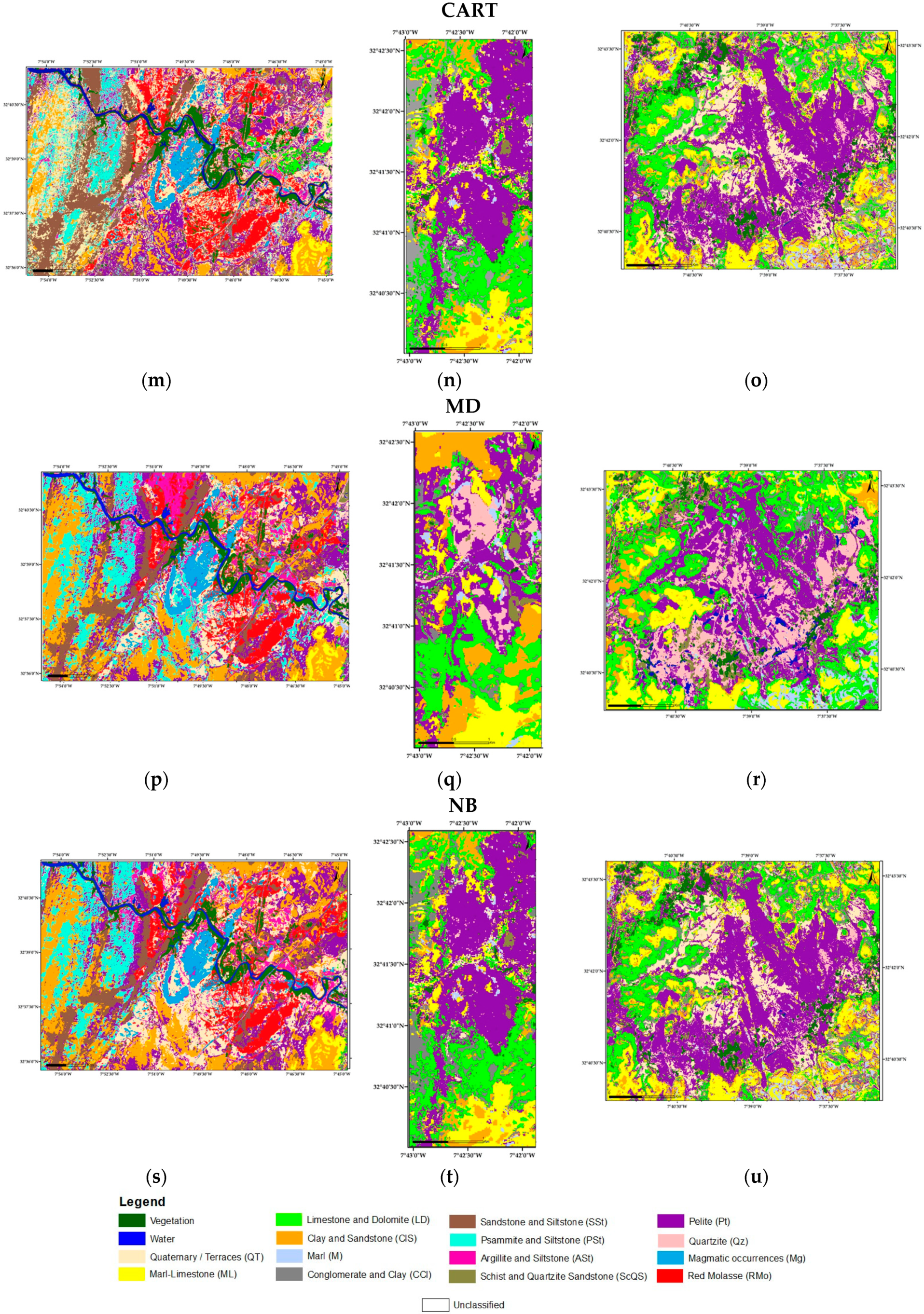
According to the statistical results summarized in Figure 7, the highest accuracies were produced using nonparametric MLAs such as SVM and RF, which were completely in line with the previous studies in this field [4,13,126], compared to parametric MLAs, namely, CART, MD and NB, as they require normally distributed data and statistical parameters are directly inferred from training datasets [125,126]. In contrast, no assumptions or statistical parameters are needed for non-parametric MLAs [130,131]. The classification findings produced in this investigation were compared with pre-existing geological maps [66] and enhanced color composite images to assess the resulting maps acquired in this study. Figure 8 shows a visual comparison between the individual classification results from our research in three complex magnified regions, particularly Machraa ben Aabou, Foum el M’jez and Oued Quibane. It can be seen in Figure 8 that basement rocks, especially pelite (Pt) (Figure 8i,h) and quartzite (Qz) (Figure 8h), were well identified using the RF algorithm. Otherwise, the SVM MLA outperformed in distinguishing different sedimentary cover rocks, namely, clay and sandstone (ClS) (Figure 8j), limestone and dolomite (LD), as well as marl–limestone (ML) (Figure 8k,l). The worst lithological maps were produced when performing classification with parametric algorithms, as illustrated in Figure 8. The mapping results of most rock units exposed in the study area using CART, MD and NB are largely misclassified into surrounding lithological units. Although the three methods achieved low classification accuracy, there were still some lithological units well identified using those algorithms. For example, the sandstone and siltstone (SSt) were well distinguished (Figure 8m,n) and achieved the highest accuracy (Figure 8a) using the CART classifier, in addition to the MD algorithm that yielded good performances in identifying the argillite and siltstone (ASt) as well as the schist and quartzite sandstone (ScQS) (Figure 7a), besides NB shows a better capability for discriminating the psammite and siltstone (PSt) (Figure 7a and Figure 8s). This further illustrated the robustness of the proposed approach in improving classification accuracy in lithological mapping by fusing multiple classifiers. Thus, adding more MLAs increases the probability that the accuracy of the proposed approach will be enhanced and higher than the highest accuracy attained by a single algorithm.
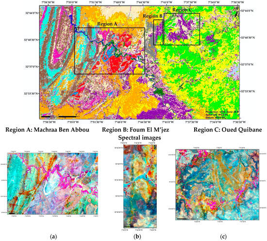


Figure 8.
Visual assessment of magnified areas among the classification results against an enhanced color composite and existing geological maps.
The spectral profile from S2 bands (Figure 5) show that the rocks composed of argillites (ASt) in addition to those composed of silicates, particularly the magmatic rocks (Mg and RMo), are more distinct compared to other lithological units’ spectra; therefore, all the MLAs discriminate them correctly. Otherwise, a lesser separability in the spectral profile is shown by sedimentary rocks composed of the following (Table 2): sandy rocks (PSt and SSt); clay (CCl and ClS); calcite and dolomite (LD); in addition to the basement rocks (Pt and Qz), their mineralogical composition is predominantly quartz, which leads to a confused discrimination in individual MLAs, especially parametric classifiers that were affected by the heterogeneity of these classes. Thus, lithological mapping using MLAs depends not only on the data quality and robustness of the classifiers but is also proportional to the nature of lithological units, their mineral compositions, their spectral separability, weatherability and the magnitude of bedrock outcrops relative to other lithological units.

Table 2.
Lithological and mineralogical description of the rock units in the study area.
Besides visual comparison with pre-existing geological data, extensive fieldwork has been performed to update and validate the results of the lithological map produced using the proposed approach. Three fieldwork missions were carried out in March 2022, by investigating the mapped area.
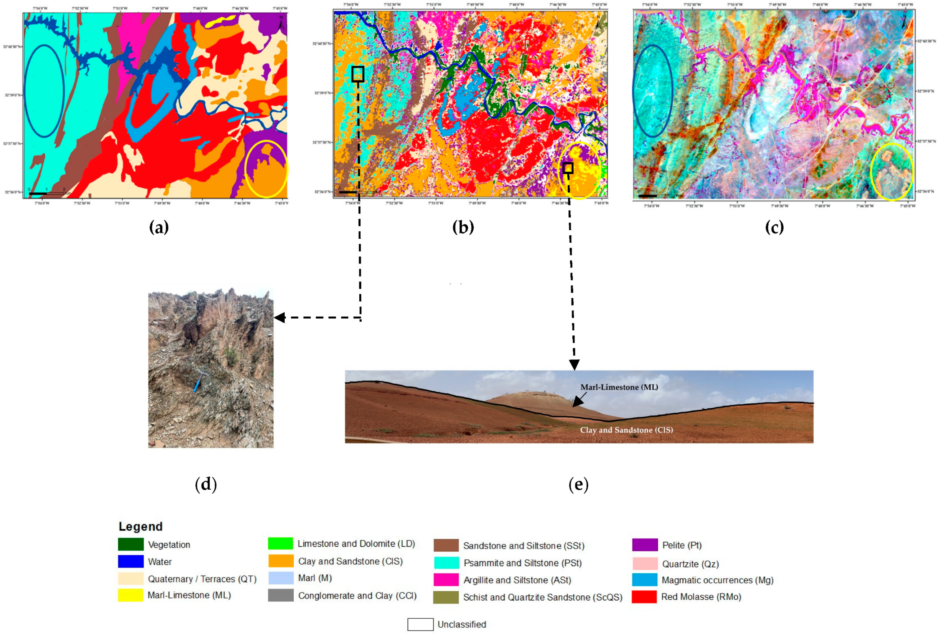
The geological map (Figure 9a) and the enhanced color composite (Figure 9c) were used along with the field investigation to validate the proposed approach (Figure 9b) in the region of Machraa ben Aabou. The folds of psammite and siltstone (PSt) and clay and sandstone (ClS) were tuned by the in-situ field verification shown in Figure 9d. Those folds are not mapped in the pre-existing geological map; however, they are observed in the color composite image and well identified in the proposed method as shown in the blue circle in Figure 9a–c. For the cover units, the geological map shows only one rock unit type, which is clay and sandstone (ClS); otherwise, the color composite image and field verification (Figure 9e) confirmed the presence of two cover-type lithologies in the resulting map, which are marl–limestone (ML) and clay and sandstone (ClS), as shown with a yellow circle in Figure 9a–c.
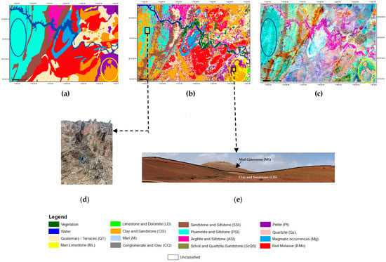
Figure 9.
Validation of the proposed approach at the magnified area of Machraa ben Aabou: (a) existing geological map; (b) lithological map using DST; (c) enhanced color composite and field photographs of (d) psammite and siltstone (PSt); (e) panoramic view of cover lithologies.
Furthermore, the geological map (Figure 10c), the enhanced color composite (Figure 10e) and the field survey performed along the complex region of Foum el M’jez (shown in Figure 10) were used to validate the optimized lithological map results using the DST approach. The verification locations show considerable compatibility with the predicted lithologies.
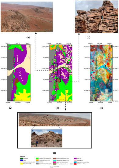
Figure 10.
Validation of the proposed approach at the magnified area of Foum el M’jez: (a) fractured limestone and dolomite (LD); (b) sandstone and siltstone (SSt); (c) existing geological map; (d) lithological map using DST; (e) enhanced color composite; (f) panoramic view of the basement outcrop with A: the Zoom to the Quartzite (Qz).
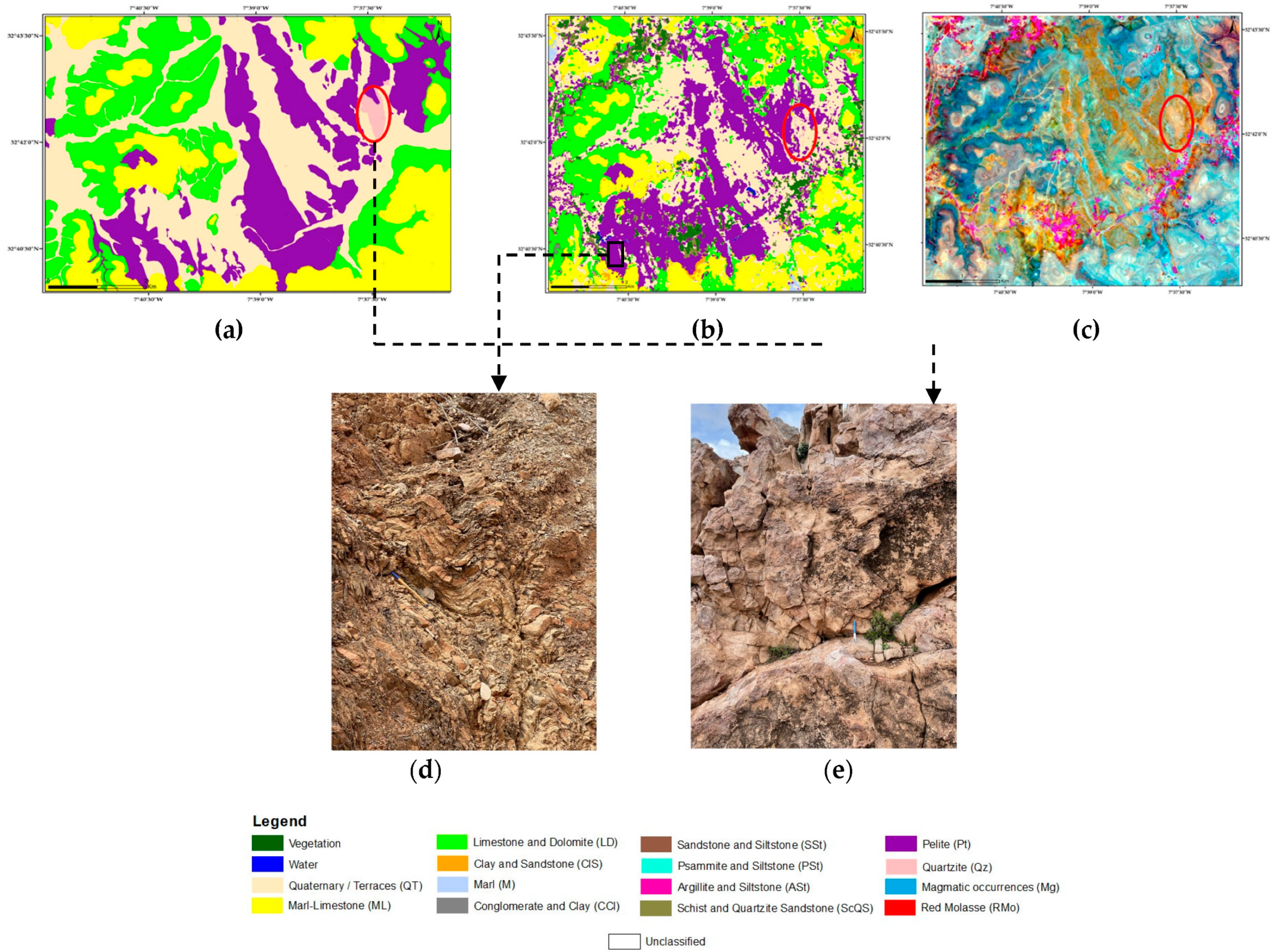
Figure 11 shows the in-situ field verification of the basement outcrops of the complex region of Oued Quibane. Additionally, through the field survey, the geological map (Figure 11a) and the enhanced color composite (Figure 11c) have been provided to validate the lithological map produced using the proposed approach. Most of the lithological units exposed in the study area are somewhat consistent and accurate; otherwise, the quartzite (Qz) exposed on surface lithology has been replaced by Quaternary/terraces (QT), as marked by red circles in Figure 11a–c, as the highest overall accuracy of the Qz lithological units achieved using RF (80%) is lower than the highest accuracy of the QT (89%) obtained using SVM MLA (Figure 7a).
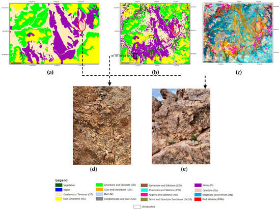
Figure 11.
Validation of the proposed approach at the magnified area of Oued Quibane: (a) existing geological map; (b) lithological map using DST; (c) enhanced color composite and field photographs of the basement outcrops: (d) pelite (Pt) and (e) quartzite (Qz).
Summarily, lithological classification of a large complex semi-arid region, such as the northern part of the Paleozoic of Rehamna in the Moroccan Meseta, is impossible to process by commonly used traditional classification software packages. Therefore, this study exploits the capabilities of cloud-based platforms jointly with local computer software to optimize lithological mapping. Based on spatio-spectral information of S2A imagery, the results reveal that the proposed approach improves the classification performance compared to individual classifiers.
6. Conclusions
Due to the complexity and limited data quality in free satellite-borne remote sensing imagery as well as the restricted performance of single classification algorithms, this study demonstrates a fused multi-classifier (SVM, RF, MD, NB) approach for optimizing lithological mapping using the DST method applied to spectral and textural information of Sentinel 2A imagery. The free cloud-based computing platform, GEE, has been proposed in order to access and process the datasets in a vast part of the study area. This process occurred in the north of the complex Paleozoic massif of Rehamna. The results demonstrate that the classification accuracy is mostly affected by the types of lithological units and their mineral compositions, variations in reflectance spectra, non-linear spectral mixing and sensitivity to weathering, in addition to the classification methods. The resulting lithological maps were compared visually and assessed statistically using the confusion matrix. The proposed DST classified map shows a high accuracy over lithological maps resulting from the other classifiers, which indicates that this approach is more robust and effective in increasing the accuracy in the lithological mapping of complex semi-arid regions due to the complementary contribution of MLAs. In future works, the lithological mapping will be based on a deep learning algorithm, which will be developed within GEE, as cloud computing services are making deep learning more accessible and easier to manage a large-scale computing capacity as well as training algorithms on a distributed architecture, which can be immensely helpful in a geological investigation.
Author Contributions
Conceptualization, I.S., M.R., M.H., B.P.; methodology, I.S., M.R., M.H., B.P., S.G., A.A., K.N.A.M., A.D.; software, I.S. and M.H.; validation with field investigations, I.S., M.R. and F.E.K.; writing original draft preparation, I.S.; review and editing, B.P., S.G., A.A., K.N.A.M., A.D.; supervision, M.R., M.H., F.E.K. and B.P.; project administration, B.P.; funding acquisition, B.P., A.A., K.N.A.M. All authors have read and agreed to the published version of the manuscript.
Funding
The study is supported by the Centre for Advanced Modelling and Geospatial Information Systems (CAMGIS), University of Technology Sydney. Moreover, partly supported by the Researchers Supporting Project, King Saud University, Riyadh, Saudi Arabia, under Grant RSP-2021/14; supported by the UKM YSDChair of Sustainability (UKM-YSD-2021-003).
Data Availability Statement
Not applicable.
Acknowledgments
The authors would like to thank the anonymous reviewers for their valuable comments on the manuscript, which helped improve the quality of the paper. We would also like to thank the Google Earth Engine team for their wonderful work and service.
Conflicts of Interest
The authors declare no conflict of interest.
References
- Ye, B.; Tian, S.; Ge, J.; Sun, Y. Assessment of WorldView-3 data for lithological mapping. Remote Sens. 2017, 9, 1132. [Google Scholar] [CrossRef]
- El Fels, A.E.A.; El Ghorfi, M. Using remote sensing data for geological mapping in semi-arid environment: A machine learning approach. Earth Sci. Inform. 2022, 15, 485–496. [Google Scholar] [CrossRef]
- Ge, W.; Cheng, Q.; Tang, Y.; Jing, L.; Gao, C. Lithological classification using Sentinel-2A data in the Shibanjing ophiolite complex in Inner Mongolia, China. Remote Sens. 2018, 10, 638. [Google Scholar] [CrossRef]
- Serbouti, I.; Raji, M.; Hakdaoui, M.; Pradhan, B.; Lee, C.W.; Alamri, A.M. Pixel and Object-Based Machine Learning Classification Schemes for Lithological Mapping Enhancement of Semi-Arid Regions Using Sentinel-2A Imagery: A Case Study of the Southern Moroccan Meseta. IEEE Access 2021, 9, 119262–119278. [Google Scholar] [CrossRef]
- Imane, S.; Mohamed, R.; Mustapha, H. A comparison of GEOBIA Vs PBIA machine learning methods for lithological mapping using Sentinel 2 imagery: Case study of Skhour Rehamna Morocco. IEEE Int. Conf. Moroc. Geomat. 2020, 2020, 2–7. [Google Scholar] [CrossRef]
- Shirmard, H.; Farahbakhsh, E.; Müller, R.D.; Chandra, R. A review of machine learning in processing remote sensing data for mineral exploration. Remote Sens. Environ. 2022, 268, 112750. [Google Scholar] [CrossRef]
- Peyghambari, S.; Zhang, Y. Hyperspectral remote sensing in lithological mapping, mineral exploration, and environmental geology: An updated review. J. Appl. Remote Sens. 2021, 15, 1–25. [Google Scholar] [CrossRef]
- Bentahar, I.; Raji, M.; Si Mhamdi, H. Fracture network mapping using Landsat-8 OLI, Sentinel-2A, ASTER, and ASTER-GDEM data, in the Rich area (Central High Atlas, Morocco). Arab. J. Geosci. 2020, 13, 16. [Google Scholar] [CrossRef]
- Mwaniki, M.W.; Matthias, M.S.; Schellmann, G. Application of Remote Sensing Technologies to Map the Structural Geology of Central Region of Kenya. IEEE J. Sel. Top. Appl. Earth Obs. Remote Sens. 2015, 8, 1855–1867. [Google Scholar] [CrossRef]
- Serbouti, M.I.; Hakdaoui, M.R. Contribution of spatial multi-sensor imagery to the cartography of structural lineaments: Case study of the paleozoic massif of rehamna (Moroccan Meseta). Earth Obs. Adv. A Chang. World 2019, 1, 122–125. [Google Scholar] [CrossRef]
- Othman, A.A.; Gloaguen, R. Improving lithological mapping by SVM classification of spectral and morphological features: The discovery of a new chromite body in the Mawat ophiolite complex (Kurdistan, NE Iraq). Remote Sens. 2014, 6, 6867–6896. [Google Scholar] [CrossRef]
- Cracknell, M.J.; Reading, A.M. Geological mapping using remote sensing data: A comparison of five machine learning algorithms, their response to variations in the spatial distribution of training data and the use of explicit spatial information. Comput. Geosci. 2014, 63, 22–33. [Google Scholar] [CrossRef]
- Bachri, I.; Hakdaoui, M.; Raji, M.; Teodoro, A.C.; Benbouziane, A. Machine learning algorithms for automatic lithological mapping using remote sensing data: A case study from Souk Arbaa Sahel, Sidi Ifni Inlier, Western Anti-Atlas, Morocco. ISPRS Int. J. Geo-Inf. 2019, 8, 248. [Google Scholar] [CrossRef]
- Van der Meer, F.D.; Van der Werff, H.M.A.; Van Ruitenbeek, F.J.A. Potential of ESA’s Sentinel-2 for geological applications. Remote Sens. Environ. 2014, 148, 124–133. [Google Scholar] [CrossRef]
- Grebby, S.; Field, E.; Tansey, K. Evaluating the use of an object-based approach to lithological mapping in vegetated terrain. Remote Sens. 2016, 8, 843. [Google Scholar] [CrossRef]
- Wei, J.; Liu, X.; Liu, J. Integrating textural and spectral features to classify silicate-bearing rocks using landsat 8 data. Appl. Sci. 2016, 6, 10. [Google Scholar] [CrossRef]
- Masoumi, F.; Eslamkish, T.; Abkar, A.A.; Honarmand, M.; Harris, J.R. Integration of spectral, thermal, and textural features of ASTER data using Random Forests classification for lithological mapping. J. African Earth Sci. 2017, 129, 445–457. [Google Scholar] [CrossRef]
- Adams, J.B.; Smith, M.O.; Johnson, P.E. Correction [to ‘Spectral mixture modeling: A new analysis of rock and soil types at the Viking Lander 1 site’ by John, B. Adams, Milton, O. Smith, and Paul, E. Johnson]. J. Geophys. Res. 1986, 91, 10513. [Google Scholar] [CrossRef]
- Drake, N.A. Reflectance spectra of evaporite minerals (400–2500 nm): Applications for remote sensing. Int. J. Remote Sens. 1995, 16, 2555–2571. [Google Scholar] [CrossRef]
- Mars, J.C.; Rowan, L.C. ASTER spectral analysis and lithologic mapping of the Khanneshin carbonatite volcano, Afghanistan. Geosphere 2011, 7, 276–289. [Google Scholar] [CrossRef]
- Shafiq, M.A.; Wang, Z.; Amin, A.; Hegazy, T.; Deriche, M.; AlRegib, G. Detection of salt-dome boundary surfaces in migrated seismic volumes using gradient of textures. SEG Tech. Progr. Expand. Abstr. 2015, 34, 1811–1815. [Google Scholar] [CrossRef]
- Ryherd, S.; Woodcock, C. Combining spectral and texture data in the segmentation of remotely sensed images. Photogramm. Eng. Remote Sens. 1996, 62, 181–194. [Google Scholar]
- Li, P.; Li, Z.; Moon, W.M. Lithological discrimination of Altun area in northwest China using Landsat TM data and geostatistical textural information. Geosci. J. 2001, 5, 293–300. [Google Scholar] [CrossRef]
- Li, N.; Zhao, H.J.; Huang, P.; Jia, G.R.; Bai, X. A novel logistic multi-class supervised classification model based on multi-fractal spectrum parameters for hyperspectral data. Int. J. Comput. Math. 2015, 92, 836–849. [Google Scholar] [CrossRef]
- Moosavi, V.; Niazi, Y. Development of hybrid wavelet packet-statistical models (WP-SM) for landslide susceptibility mapping. Landslides 2016, 13, 97–114. [Google Scholar] [CrossRef]
- Farahbakhsh, E.; Chandra, R.; Olierook, H.K.; Scalzo, R.; Clark, C.; Reddy, S.M.; Müller, R.D. Computer vision-based framework for extracting tectonic lineaments from optical remote sensing data. Int. J. Remote Sens. 2020, 41, 760–1787. [Google Scholar] [CrossRef]
- Cross, G.R.; Jain, A.K. Markov Random Field Texture Models. IEEE Trans. Pattern Anal. Mach. Intell. 1983, 1, 25–39. [Google Scholar] [CrossRef]
- Li, N.; Frei, M.; Altermann, W. Textural and knowledge-based lithological classification of remote sensing data in Southwestern Prieska sub-basin, Transvaal Supergroup, South Africa. J. African Earth Sci. 2011, 60, 237–246. [Google Scholar] [CrossRef]
- Fuentes, I.; Padarian, J.; Iwanaga, T.; Vervoort, R.W. 3D lithological mapping of borehole descriptions using word embeddings. Comput. Geosci. 2020, 141, 104516. [Google Scholar] [CrossRef]
- Mering, C.; Chopin, F. Granulometric maps from high resolution satellite images. Image Anal. Stereol. 2002, 21, 19–24. [Google Scholar] [CrossRef]
- Chen, D.; Stow, D.A.; Gong, P. Examining the effect of spatial resolution and texture window size on classification accuracy: An urban environment case. Int. J. Remote Sens. 2004, 25, 2177–2192. [Google Scholar] [CrossRef]
- Lloyd, C.D.; Berberoglu, S.; Curran, P.J.; Atkinson, P.M. A comparison of texture measures for the per-field classification of Mediterranean land cover. Int. J. Remote Sens. 2004, 25, 3943–3965. [Google Scholar] [CrossRef]
- Tai-feng, D. Application of GLCM-Based Texture Features to Remote Sensing Image Classification. Geol. Explor. 2011, 47, 456–467. [Google Scholar]
- Emran, A.; Hakdaoui, M.; Chorowicz, J. Anomalies on geologic maps from multispectral and textural classification: The Bleida Mining District (Morocco). Remote Sens. Environ. 1996, 57, 13–21. [Google Scholar] [CrossRef]
- Puissant, A.; Hirsch, J.; Weber, C. The utility of texture analysis to improve per-pixel classification for high to very high spatial resolution imagery. Int. J. Remote Sens. 2005, 26, 73–745. [Google Scholar] [CrossRef]
- Berberoglu, S.; Lloyd, C.D.; Atkinson, P.M.; Curran, P.J. The integration of spectral and textural information using neural networks for land cover mapping in the Mediterranean. Comput. Geosci. 2000, 26, 385–396. [Google Scholar] [CrossRef]
- Merembayev, T.; Kurmangaliyev, D.; Bekbauov, B.; Amanbek, Y. A Comparison of Machine Learning Algorithms in Predicting Lithofacies: Case Studies from Norway and Kazakhstan. Energies 2021, 14, 1896. [Google Scholar] [CrossRef]
- Alajlan, N.; Bazi, Y.; Melgani, F.; Yager, R.R. Fusion of supervised and unsupervised learning for improved classification of hyperspectral images. Inf. Sci. 2012, 217, 39–55. [Google Scholar] [CrossRef]
- Dibs, H.; Hasab, H.A.; Al-Rifaie, J.K.; Al-Ansari, N. An Optimal Approach for Land-Use / Land-Cover Mapping by Integration and Fusion of Multispectral Landsat OLI Images: Case Study in Baghdad, Iraq. Water. Air. Soil Pollut. 2020, 231, 9. [Google Scholar] [CrossRef]
- Dibs, H.; Hasab, H.A.; Mahmoud, A.S.; Al-Ansari, N. Fusion Methods and Multi-classifiers to Improve Land Cover Estimation Using Remote Sensing Analysis. Geotech. Geol. Eng. 2021, 39, 5825–5842. [Google Scholar] [CrossRef]
- Shmuel, A.; Heifetz, E. Global Wildfire Susceptibility Mapping Based on Machine Learning Models. Forests 2022, 13, 1050. [Google Scholar] [CrossRef]
- Alonso-Betanzos, A.; Fontenla-Romero, O.; Guijarro-Berdiñas, B.; Hernández-Pereira, E.; Andrade, M.I.P.; Jiménez, E. An intelligent system for forest fire risk prediction and fire fighting management in Galicia. Expert Syst. Appl. 2003, 25, 545–554. [Google Scholar] [CrossRef]
- López-caloca, A.A. Data Fusion Approach for Employing Multiple Classifiers to Improve Lake Shoreline Analysis. Iberoam. Congr. Pattern Recognit. 2014, 2014, 1022–1029. [Google Scholar]
- Du, P.; Liu, S.; Xia, J.; Zhao, Y. Information fusion techniques for change detection from multi-temporal remote sensing images. Inf. Fusion 2013, 14, 19–27. [Google Scholar] [CrossRef]
- Shafer, G. A Mathematical Theory of Evidence; Princeton University Press: Princeton, NJ, USA, 1976. [Google Scholar] [CrossRef]
- Zeng, Y.; Zhang, J.; Van Genderen, J.L. Comparison and Analysis of Remote Sensing Data Fusion Techniques. Comm. Remote Sens. Pixels Process. 2006, 36, 5. [Google Scholar]
- Jiang, D.; Zhuang, D.; Huang, Y.; Fu, J. Survey of Multispectral Image Fusion Techniques in Remote Sensing Applications. Image Fusion Its Appl. 2011, 1, 1–23. [Google Scholar] [CrossRef]
- Rottensteiner, F.; Trinder, J.; Clode, S.; Kubik, K. Using the Dempster-Shafer method for the fusion of LIDAR data and multi-spectral images for building detection. Inf. Fusion 2005, 6, 283–300. [Google Scholar] [CrossRef]
- Denœux, T. A k-Nearest Neighbor Classification Rule Based on Dempster-Shafer Theory. IEEE Trans. Syst. Man. Cybern. 1995, 25, 804–813. [Google Scholar] [CrossRef]
- Fontani, M.; Bianchi, T.; De Rosa, A.; Piva, A.; Barni, M. A Dempster-Shafer framework for decision fusion in image forensics. In 2011 IEEE International Workshop on Information Forensics and Security; IEEE: Piscataway, NJ, USA, 2011. [Google Scholar] [CrossRef]
- Singh, R.; Vatsa, M.; Noore, A.; Singh, S.K. Dempster-Shafer Theory Based Classifier Fusion for Improved Fingerprint Verification Performance. In Computer Vision, Graphics and Image Processing; Springer: Berlin, Germany, 2006; pp. 941–949. [Google Scholar] [CrossRef]
- Malpica, J.A.; Alonso, M.C.; Sanz, M.A. Dempster-Shafer Theory in geographic information systems: A survey. Expert Syst. Appl. 2007, 32, 47–55. [Google Scholar] [CrossRef]
- Gorelick, N.; Hancher, M.; Dixon, M.; Ilyushchenko, S.; Thau, D.; Moore, R. Google Earth Engine: Planetary-scale geospatial analysis for everyone. Remote Sens. Environ. 2017, 202, 18–27. [Google Scholar] [CrossRef]
- Yang, L.; Driscol, J.; Sarigai, S.; Wu, Q.; Chen, H.; Lippitt, C.D. Lippitt, Google Earth Engine and Artificial Intelligence (AI): A Comprehensive Review. Remote Sens. 2022, 14, 3253. [Google Scholar] [CrossRef]
- Kumar, L.; Mutanga, O. Google Earth Engine applications since inception: Usage, trends, and potential. Remote Sens. 2018, 10, 1509. [Google Scholar] [CrossRef]
- Tamiminia, H.; Salehi, B.; Mahdianpari, M.; Quackenbush, L.; Adeli, S.; Brisco, B. Google Earth Engine for geo-big data applications: A meta-analysis and systematic review. J. Photogramm. Remote Sens. 2020, 164, 152–170. [Google Scholar] [CrossRef]
- Mondal, P.; Liu, X.; Fatoyinbo, T.E.; Lagomasino, D. Evaluating combinations of sentinel-2 data and machine-learning algorithms for mangrove mapping in West Africa. Remote Sens. 2019, 11, 2928. [Google Scholar] [CrossRef]
- Shafizadeh-Moghadam, H.; Khazaei, M.; Alavipanah, S.K.; Weng, Q. Google Earth Engine for large-scale land use and land cover mapping: An object-based classification approach using spectral, textural and topographical factors. GIScience Remote Sens. 2021, 58, 914–928. [Google Scholar] [CrossRef]
- Xiong, J.; Thenkabail, P.S.; Gumma, M.K.; Teluguntla, P.; Poehnelt, J.; Congalton, R.G. Automated cropland mapping of continental Africa using Google Earth Engine cloud computing. J. Photogramm. Remote Sens. 2017, 126, 225–244. [Google Scholar] [CrossRef]
- Yancho, J.M.M.; Jones, T.G.; Gandhi, S.R.; Ferster, C.; Lin, A.; Glass, L. The Google Earth Engine Mangrove Mapping Methodology (GEEMMM). Remote Sens. 2020, 12, 3758. [Google Scholar] [CrossRef]
- Wang, C.; Jia, M.; Chen, N.; Wang, W. Long-term surface water dynamics analysis based on landsat imagery and the Google Earth Engine Platform: A case study in the middle Yangtze River Basin. Remote Sens. 2018, 10, 1635. [Google Scholar] [CrossRef]
- Ji, H.; Li, X.; Wei, X.; Liu, W.; Zhang, L.; Wang, L. Mapping 10-m resolution rural settlements using multi-source remote sensing datasets with the google earth engine platform. Remote Sens. 2020, 12, 2832. [Google Scholar] [CrossRef]
- Pericak, A.A.; Thomas, C.J.; Kroodsma, D.A.; Wasson, M.F.; Ross, M.R.; Clinton, N.E. Mapping the yearly extent of surface coal mining in central appalachia using landsat and google earth engine. PLoS ONE 2018, 13, 0197758. [Google Scholar] [CrossRef]
- Ding, Y.; Yang, X.; Jin, H.; Wang, Z.; Liu, Y.; Liu, B. Monitoring coastline changes of the malay islands based on google earth engine and dense time-series remote sensing images. Remote Sens. 2021, 13, 3842. [Google Scholar] [CrossRef]
- Kumar, H.; Karwariya, S.K.; Kumar, R. Google Earth Engine-Based Identification of Flood Extent and Flood-Affected Paddy Rice Fields Using Sentinel-2 MSI and Sentinel-1 SAR Data in Bihar State, India. J. Indian Soc. Remote Sens. 2022, 50, 791–803. [Google Scholar] [CrossRef]
- Kamel, E.l. Géologie du Paléozoïque des Rehamna Nord-Orientaux, Maroc. Evolution Sédimentaire et Structuration Hercynienne d’un Bassin Dévono-Carbonifère Sédimentation et Déformation des Molasses Post-Orogénique; Université Paul Cézanne-Aix-Marseille III: Aix-en-Provence, France, 1987. [Google Scholar]
- Gigout, M. Etudes géologiques sur la Meseta marocaine occidentale. Notes Mém. Serv. Géol. Maroc 1951, 86, 1. [Google Scholar]
- Michard, A.; Hoepffner, C.; Jenny, P. Le couloir de cisaillement caledono-hercynien de la Meseta occidentale sur la transversale de Mechra-Ben-Abbou (Rehamna, Maroc). Bull. Société Géologique Fr. 1978, 7, 889–894. [Google Scholar] [CrossRef]
- Kamel, F.E.L.; Hassani, A.E.L. Étapes de la structuration et de la sédimentation du bassin viséen de Mechra ben Abbou (Meseta occidentale marocaine). Geodiversitas 2006, 28, 14. [Google Scholar]
- El Hassani, A.; El Kamel, F. Tectonic control of Devonian reef building in Mechra ben Abou area (northen Rehamna, Morocco). In Proceedings of the Subcommission on Devonian Stratigraphy (SDS)—IGCP 421 Morocco Meeting; Tahiri, A., El Hassani, A., Eds.; Travaux de l’Institut Scientifique: Rabat, Morocco, 2000; Volume 20, pp. 25–30. [Google Scholar]
- ASSA, R.R. Etude Géologique de la Partie Occidentale du Massif hercynien des Rehamna Septentrionales (Meseta Marocaine). In Lithostratigraphie, Plissements et Métamorphisme, Chevauchements et Nappes; Université de Droit, D’économie et des Sciences D’aix-Marseille: Aix en Provence, France, 1984. [Google Scholar]
- Chastain, R.; Housman, I.; Goldstein, J.; Finco, M.; Tenneson, K. Empirical cross sensor comparison of Sentinel-2A and 2B MSI, Landsat-8 OLI, and Landsat-7 ETM+ top of atmosphere spectral characteristics over the conterminous United States. Remote Sens. Environ. 2019, 221, 274–285. [Google Scholar] [CrossRef]
- Immitzer, M.; Vuolo, F.; Atzberger, C. First experience with Sentinel-2 data for crop and tree species classifications in central Europe. Remote Sens. 2016, 8, 166. [Google Scholar] [CrossRef]
- Baetens, L.; Desjardins, C.; Hagolle, O. Validation of copernicus Sentinel-2 cloud masks obtained from MAJA, Sen2Cor, and FMask processors using reference cloud masks generated with a supervised active learning procedure. Remote Sens. 2019, 11, 433. [Google Scholar] [CrossRef]
- Hotelling, H. Analysis of a complex of statistical variables into Principal Components. J. Educ. Psychol. 1933, 24, 417–441. [Google Scholar] [CrossRef]
- Zhang, X.; Pazner, M.; Duke, N. Lithologic and mineral information extraction for gold exploration using ASTER data in the south Chocolate Mountains (California). J. Photogramm. Remote Sens. 2007, 62, 271–282. [Google Scholar] [CrossRef]
- Khalifa, A.; Bashir, B.; Çakir, Z.; Kaya, Ş.; Alsalman, A.; Henaish, A. Paradigm of geological mapping of the adıyaman fault zone of eastern turkey using landsat 8 remotely sensed data coupled with pca, ica, and mnfa techniques. Int. J. Geo-Inf. 2021, 10, 368. [Google Scholar] [CrossRef]
- Jansson, N.F.; Allen, R.L.; Skogsmo, G.; Tavakoli, S. Principal component analysis and K-means clustering as tools during exploration for Zn skarn deposits and industrial carbonates, Sala area, Sweden. J. Geochemical Explor. 2022, 233, 106909. [Google Scholar] [CrossRef]
- Pearson, K. LIII. On lines and planes of closest fit to systems of points in space. Philos. Mag. J. Sci. 1901, 2, 559–572. [Google Scholar] [CrossRef]
- Jolliffe, I.T. Principal Component Analysis, Second Edition. Encycl. Stat. Behav. Sci. 2002, 30, 487. [Google Scholar] [CrossRef]
- RAmer, R.; Kusky, T.; Ghulam, A. Lithological mapping in the Central Eastern Desert of Egypt using ASTER data. J. Afr. Earth Sci. 2010, 56, 75–82. [Google Scholar] [CrossRef]
- Priyadarshini, K.N.; Sivashankari, V.; Shekhar, S.; Balasubramani, K. Comparison and Evaluation of Dimensionality Reduction Techniques for Hyperspectral Data Analysis. Multidiscip. Digit. Publ. Inst. Proc. 2019, 24, 6. [Google Scholar] [CrossRef]
- Nielsen, A.A. Kernel maximum autocorrelation factor and minimum noise fraction transformations. IEEE Trans. Image Process. 2011, 20, 612–624. [Google Scholar] [CrossRef]
- Bjorgan, A.; Randeberg, L.L. Real-time noise removal for line-scanning hyperspectral devices using a minimum noise fraction-based approach. Sensors 2015, 15, 3362–3378. [Google Scholar] [CrossRef]
- Lee, J.B.; Woodyatt, A.S.; Berman, M. Enhancement of High Spectral Resolution Remote-Sensing Data by a Noise-Adjusted Principal Components Transform. IEEE Trans. Geosci. Remote Sens. 1990, 28, 295–304. [Google Scholar] [CrossRef]
- Green, A.A.; Berman, M.; Switzer, P.; Craig, M.D. A Transformation for Ordering Multispectral Data in Terms of Image Quality with Implications for Noise Removal. IEEE Trans. Geosci. Remote Sens. 1988, 26, 65–74. [Google Scholar] [CrossRef]
- Gurugnanam, B.; Arulbalaji, P.; Midhuna, V.; Kumaravel, S. Lithological Discrimination of Anorthosite using ASTER data in Oddanchatram Area, Dindigul district, Tamil Nadu, India. Int. J. Adv. Eng. Manag. Sci. 2017, 3, 316–324. [Google Scholar] [CrossRef]
- Kumar, C.; Shetty, A.; Raval, S.; Sharma, R.; Ray, P.C. Lithological Discrimination and Mapping using ASTER SWIR Data in the Udaipur area of Rajasthan, India. Procedia Earth Planet. Sci. 2015, 11, 180–188. [Google Scholar] [CrossRef]
- Luo, G.; Chen, G.; Tian, L.; Qin, K.; Qian, S.E. Minimum Noise Fraction versus Principal Component Analysis as a Preprocessing Step for Hyperspectral Imagery Denoising. Can. J. Remote Sens. 2016, 42, 106–116. [Google Scholar] [CrossRef]
- Kupidura, P. The comparison of different methods of texture analysis for their efficacy for land use classification in satellite imagery. Remote Sens. 2019, 11, 1233. [Google Scholar] [CrossRef]
- Wulder, M.; Boots, B. Local spatial autocorrelation characteristics of remotely sensed imagery assessed with the Getis statistic. Int. J. Remote Sens. 1998, 19, 2223–2231. [Google Scholar] [CrossRef]
- Dekker, R.J. Texture analysis and classification of ERS SAR images for map updating of urban areas in The Netherlands. IEEE Trans. Geosci. Remote Sens. 2003, 41, 1950–1958. [Google Scholar] [CrossRef]
- Myint, S.W.; Gober, P.; Brazel, A.; Grossman-Clarke, S.; Weng, Q. Per-pixel vs. object-based classification of urban land cover extraction using high spatial resolution imagery. Remote Sens. Environ. 2011, 115, 1145–1161. [Google Scholar] [CrossRef]
- Pelz, J.B. Morphological image segmentation by local granulometric size distributions. J. Electron. Imaging 1992, 1, 46. [Google Scholar] [CrossRef]
- Breiman, L. Random forests. Mach. Learn. 2001, 45, 5–32. [Google Scholar] [CrossRef]
- Breiman, L. Bagging Predictors. Mach. Learn. 1996, 24, 123–140. [Google Scholar] [CrossRef]
- Waske, B.; Braun, M. Classifier ensembles for land cover mapping using multitemporal SAR imagery. ISPRS J. Photogramm. Remote Sens. 2009, 64, 450–457. [Google Scholar] [CrossRef]
- Breiman, C.J.; Friedman, L.; Olshen, J.H.; Stone, R.A. Classification and Regression Trees, 1st ed.; Chapman ve Hall: Pacific Grove, CA, USA, 1984. [Google Scholar] [CrossRef]
- Kuhn, S.; Cracknell, M.J.; Reading, A.M. Lithologic mapping using Random Forests applied to geophysical and remote-sensing data: A demonstration study from the Eastern Goldfields of Australia. Geophysics 2018, 83, B183–B193. [Google Scholar] [CrossRef]
- Albert, G.; Ammar, S. Application of random forest classification and remotely sensed data in geological mapping on the Jebel Meloussi area (Tunisia). Arab. J. Geosci. 2021, 14, 2240. [Google Scholar] [CrossRef]
- Vapnik, V.N. The Nature of Statistical Learning; Springer Science & Business Media: New York, NY, USA, 1995. [Google Scholar]
- Petropoulos, G.P.; Kalaitzidis, C.; Vadrevu, K.P. Support vector machines and object-based classification for obtaining land-use/cover cartography from Hyperion hyperspectral imagery. Comput. Geosci. 2012, 41, 99–107. [Google Scholar] [CrossRef]
- Huang, C.; Davis, L.S.; Townshend, J.R.G. International Journal of Remote Sensing An assessment of support vector machines for land cover classification An assessment of support vector machines for land cover classi cation. Int. J. Remote Sens. 2002, 23, 725–749. [Google Scholar] [CrossRef]
- Srivastava, P.K.; Han, D.; Rico-Ramirez, M.A.; Bray, M.; Islam, T. Selection of classification techniques for land use/land cover change investigation. Adv. Sp. Res. 2012, 50, 1250–1265. [Google Scholar] [CrossRef]
- Shebl, A.; Abdellatif, M.; Hissen, M.; Abdelaziz, M.I.; Csámer, Á. Lithological mapping enhancement by integrating Sentinel 2 and gamma-ray data utilizing support vector machine: A case study from Egypt. Int. J. Appl. Earth Obs. Geoinf. 2021, 105, 102619. [Google Scholar] [CrossRef]
- Breiman, L.; Friedman, J.H.; Olshen, R.A.; Stone, C.J. Classification and Regression Trees, 1st ed.; Chapman & Hall: London, UK; New York, NY, USA; Washington, DC, USA, 1984. [Google Scholar]
- Farris, F.A. The gini index and measures of inequality. Am. Math. Mon. 2010, 117, 851–864. [Google Scholar] [CrossRef]
- Cracknell, M.J. Machine Learning for Geological Mapping: Algorithms and Applications; University of Tasmania: Hobart, Australia, 2014. [Google Scholar]
- Pal, M.; Rasmussen, T.; Porwal, A. Optimized Lithological Mapping from Multispectral and Hyperspectral Remote Sensing Images Using Fused Multi-Classifiers. Remote Sens. 2020, 12, 177. [Google Scholar] [CrossRef]
- Gemusse, U.; Lima, A.; Teodoro, A. Comparing different techniques of satellite imagery classification to mineral mapping pegmatite of Muiane and Naipa: Mozambique). In Earth Resources and Environmental Remote Sensing/GIS Applications X; SPIE: Bellingham, DC, USA, 2019; pp. 270–279. [Google Scholar] [CrossRef]
- Kruse, F.A.; Perry, S.L. Mineral mapping using simulated worldview-3 short-wave-infrared imagery. Remote Sens. 2013, 5, 2688–2703. [Google Scholar] [CrossRef]
- Richards, J.A. Classification and Regression Trees, 5th ed.; Springer: Berlin/Heidelberg, Germany, 2013. [Google Scholar] [CrossRef]
- Minskyt, M. Steps toward artificial intelligence. Proc. IRE 1961, 49, 8–30. [Google Scholar] [CrossRef]
- Maron, M.E. Automatic indexing: An experimental inquiry. J. Assoc. Comput. Mach. 1961, 8, 404–417. [Google Scholar] [CrossRef]
- Hastie, T.; Tibshirani, R.; Friedman, J. The Elements of Statistical Learning, 2nd ed.; Springer: New York, NY, USA, 2008. [Google Scholar]
- Domingos, M.; Pazzani, P. On the Optimality of the Simple Bayesian Classifier under Zero-One Loss. Mach. Learn. 1997, 29, 103–130. [Google Scholar] [CrossRef]
- Dumais, S.; Platt, J.; Heckerman, D.; Sahami, M. Inductive learning algorithms and representations for text categorization. In Proceedings of the 3rd International Conference on Information and Knowledge Management, Bethesda, MD, USA, 1 November 1998; pp. 148–155. [Google Scholar]
- Molina, R.; De la Blanca, N.P.; Taylor, C.C. Modern statistical techniques. In Machine Learning, Neural and Statistical Classification; Chichester, E.H., Michie, D., Spiegelhalter, D., Taylor, C.C., Eds.; Ellis Horwood: Chichester, UK, 1994; pp. 29–49. [Google Scholar] [CrossRef]
- Bloch, I.; Maitre, H. Fusion de données en traitement d’images: Modèles d’information et de décision. Trait. Du Signal 1994, 11, 435–446. [Google Scholar]
- Taleb-Ahmed, A.; Gautier, L.; Rombaut, M. Architecture de fusion de données basée sur la théorie de l’évidence pour la reconstruction d’ une vertèbre Structure of data fusion based on the theory of evidence for the reconstruction of vertebra. Trait. Signal 2002, 19, 267–283. [Google Scholar]
- Feizizadeh, B. A Novel Approach of Fuzzy Dempster-Shafer Theory for Spatial Uncertainty Analysis and Accuracy Assessment of Object-Based Image Classification. IEEE Geosci. Remote Sens. Lett. 2018, 15, 18–22. [Google Scholar] [CrossRef]
- Zhang, W.; Deng, Y. Combining conflicting evidence using the DEMATEL method. Soft Comput. 2019, 23, 8207–8216. [Google Scholar] [CrossRef]
- Yuan, K.; Deng, Y. Conflict evidence management in fault diagnosis. Int. J. Mach. Learn. Cybern. 2017, 10, 121–130. [Google Scholar] [CrossRef]
- Klir, M.W.G. Uncertainty-Based Information: Elements of Generalized Information Theory; Springer Science & Business Media: Berlin, Germany, 2003; Volume 184, Available online: http://link.springer.com/10.1007/978-3-7908-1869-7 (accessed on 19 September 2022).
- Ma, L.; Cheng, L.; Li, M.; Liu, Y.; Ma, X. Training set size, scale, and features in Geographic Object-Based Image Analysis of very high resolution unmanned aerial vehicle imagery. J. Photogramm. Remote Sens. 2015, 102, 14–27. [Google Scholar] [CrossRef]
- Serbouti, I.; Raji, M.; Hakdaoui, M. Lithological Mapping for a Semi-arid Area Using GEOBIA and PBIA Machine Learning Approaches with Sentinel-2 Imagery: Case Study of Skhour Rehamna, Morocco. In Geospatial Intelligence; Barramou, F., El Brirchi, E.H., Mansouri, K., Dehbi, Y., Eds.; Advances in Science, Technology & Innovation; Springer: Cham, Switzerland, 2022. [Google Scholar] [CrossRef]
- Adiri, Z.; El Harti, A.; Jellouli, A.; Maacha, L.; Bachaoui, E.M. Lithological mapping using Landsat 8 OLI and Terra2016.pdf. J. Appl. Remote Sens. 2016, 10, 016005. [Google Scholar] [CrossRef]
- Grebby, S.; Naden, J.; Cunningham, D.; Tansey, K. Integrating airborne multispectral imagery and airborne LiDAR data for enhanced lithological mapping in vegetated terrain. Remote Sens. Environ. 2011, 115, 214–226. [Google Scholar] [CrossRef]
- Bentahar, I.; Raji, M. Comparison of Landsat OLI, ASTER, and Sentinel 2A data in lithological mapping: A Case study of Rich area (Central High Atlas, Morocco). Adv. Sp. Res. 2021, 67, 945–963. [Google Scholar] [CrossRef]
- Wieland, M.; Pittore, M. Performance evaluation of machine learning algorithms for urban pattern recognition from multi-spectral satellite images. Remote Sens. 2014, 6, 2912–2939. [Google Scholar] [CrossRef]
- Abedi, R. Comparison of Parametric and Non-Parametric Techniques to Accurate Classification of Forest Attributes on Satellite Image Data. J. Environ. Sci. Stud. 2021, 5, 3229–3235. [Google Scholar]
Publisher’s Note: MDPI stays neutral with regard to jurisdictional claims in published maps and institutional affiliations. |
© 2022 by the authors. Licensee MDPI, Basel, Switzerland. This article is an open access article distributed under the terms and conditions of the Creative Commons Attribution (CC BY) license (https://creativecommons.org/licenses/by/4.0/).

