Abstract
Combinations of multi-sensor remote sensing images and machine learning have attracted much attention in recent years due to the spectral similarity of wetland plant canopy. However, the integration of hyperspectral and quad-polarization synthetic aperture radar (SAR) images for classifying marsh vegetation has still been faced with the challenges of using machine learning algorithms. To resolve this issue, this study proposed an approach to classifying marsh vegetation in the Honghe National Nature Reserve, northeast China, by combining backscattering coefficient and polarimetric decomposition parameters of C-band and L-band quad-polarization SAR data with hyperspectral images. We further developed an ensemble learning model by stacking Random Forest (RF), CatBoost and XGBoost algorithms for marsh vegetation mapping and evaluated its classification performance of marsh vegetation between combinations of hyperspectral and full-polarization SAR data and any of the lone sensor images. Finally, this paper explored the effect of different polarimetric decomposition methods and wavelengths of radar on classifying wetland vegetation. We found that a combination of ZH-1 hyperspectral images, C-band GF-3, and L-band ALOS-2 quad-polarization SAR images achieved the highest overall classification accuracy (93.13%), which was 5.58–9.01% higher than that only using C-band or L-band quad-polarization SAR images. This study confirmed that stacking ensemble learning provided better performance than a single machine learning model using multi-source images in most of the classification schemes, with the overall accuracy ranging from 77.02% to 92.27%. The CatBoost algorithm was capable of identifying forests and deep-water marsh vegetation. We further found that L-band ALOS-2 SAR images achieved higher classification accuracy when compared to C-band GF-3 polarimetric SAR data. ALOS-2 was more sensitive to deep-water marsh vegetation classification, while GF-3 was more sensitive to shallow-water marsh vegetation mapping. Finally, scattering model-based decomposition provided important polarimetric parameters from ALOS-2 SAR images for marsh vegetation classification, while eigenvector/eigenvalue-based and two-component decompositions produced a great contribution when using GF-3 SAR images.
1. Introduction
Wetlands are one of the most important and productive ecosystems on Earth [1], providing habitat for highly endangered wildlife and an important function for nutrient cycling and climate change mitigation [2]. Wetland vegetation is the most direct indicator of wetland degradation and succession. The distribution pattern and growth status of vegetation play an essential role in the stability of wetland ecosystems [3]. Due to human activities and natural factors, the global marshland ecosystems have suffered different degrees of destruction in the past decades and causing wetland vegetation degradation and shrinkage or even disappearance [4,5,6]. It is an important prerequisite for wetland management and protection to obtain a high-precision classification of wetland vegetation [7,8]. Due to difficult access, traditional field surveys are time-consuming, scale-limited, and dangerous [9,10]. Therefore, remote sensing technology has been considered an indispensable approach to conducting large-scale wetland vegetation monitoring and mapping with high spatial and temporal resolution [11,12].
However, it is difficult to precisely identify marsh vegetation with limited spectral bands due to the vegetational spectral similarity. Hyperspectral images with rich spectral information have been used for wetland vegetation classification [13,14]. Sun et al. [15] used the Ziyuan-02D hyperspectral images to map coastal wetlands, and the classification accuracy of China’s Yellow River Delta and Yancheng coastal wetlands can reach 96.92% and 94.84%, respectively. Liu et al. [16] used the complementary advantages of hyperspectral images (high spectral resolution) and multispectral images (high spatial resolution) to achieve effective vegetation classification of coastal swamps. Although hyperspectral images have abundant spectral information, it is necessary to conduct data dimension reduction and variable selection because of information redundancy. Moreover, Hyperspectral images are easily affected by clouds, fog, and rainy weather and have weak penetration capabilities of vegetation canopy [17]. Therefore, only using Hyperspectral images cannot effectively identify and monitor wetland vegetation. Nonetheless, Radar sensors are not disturbed by clouds and rain and can penetrate the vegetation canopy. Previous studies have confirmed that synthetic aperture radar (SAR) images could identify submerged herbaceous vegetation [18]. Polarimetric SAR images can provide more abundant scattering information and enhance the separability of wetland vegetation [19,20]. However, most traditional studies on wetland classification have usually used single-polarization or dual-polarization SAR images, which have challenges in fine classifications due to the limited information about the scattering mechanism of the target. With the development of high-resolution SAR technology, quad-polarization SAR data has been gradually applied to wetland vegetation extraction [21,22]. The scattering types of wetlands are very complex and diverse. Compared with single-polarization or dual-polarization data, quad-polarization SAR sensors can present more information about the scattering characteristics of vegetation and further improve the classification accuracy of wetland vegetation. The wavelength (frequency) influences the penetrability of SAR to the surface and vegetation, and combinations of multi-frequency and multi-polarization SAR data have been an effective approach for wetland mapping [8]. Mahdianpari et al. [23] used X-band single-polarization TerraSAR, L-band dual-polarization ALOS-2, and C-band quad-polarization RADARSAT-2 to classify marsh and finally achieved 94% overall classification accuracy. Evans and Costa [24] used multi-temporal L-band ALOS/PALSAR, C-band RADARSAT-2, and ENVISAT/ASAR to conduct six wetlands vegetation habitats mapping. Only using optical or SAR data for wetland classification is difficult to achieve desirable results due to spectral similarity and canopy structure diversity [25,26]. Therefore, several scholars attempted to integrate optical and SAR images for vegetation mapping. Erinjery et al. [27] effectively improved the classification accuracy of tropical rainforests in the Western Ghats by integrating Sentinel-1 SAR data and Sentinel-2 multispectral images. Tu et al. [28] classified vegetation in the Yellow River Delta by combing ZH-1 hyperspectral images and C-band GF-3 quad-polarization SAR images, which confirmed that the synergistic use of multi-source data produced a higher classification accuracy than only using single GF-3 or ZH-1 image. However, few scholars have explored the effect of combining different wavelengths of quad-polarization SAR data with hyperspectral images on marsh vegetation mapping.
Machine learning (ML) algorithms (such as Random Forest (RF), Decision Tree, Support Vector Machine, XGBoost, etc.) have become one of the important methods for wetland vegetation mapping [29,30,31,32,33]. Beijma et al. used the RF algorithm for vegetation classification of Llanrhidian salt marshes in the UK and achieved a classification accuracy of 64.90–91.90% [34]. Although these results demonstrated that a single ML algorithm could achieve high-accuracy wetland vegetation mapping, the classification ability of a single ML algorithm is not stable for different data combinations and different wetland scenes. To resolve this issue, various ensemble learning algorithms and techniques have been proposed. It was found that the new model derived from multiple classifiers has a greater generalization ability and better classification performance [35]. Stacking is an ensemble learning algorithm that aggregates the outputs of multiple base models to train the metamodel, improve classification accuracy and enhance model stability [36]. Previous studies reported that wetland classifications based on Stacking were better than a single ML classifier [37,38]. However, there is still a lack of systematic demonstration of the performance of the Stacking algorithm in marsh vegetation classification using the integration of hyperspectral and multi-frequency quad-polarization SAR data.
To fill the gaps in previous studies, this paper aims to combine spaceborne hyperspectral, multi-frequency (C-band and L-band) quad-polarization SAR images to classify marsh vegetation in Honghe National Nature Reserve, northeast China using stacking ensemble learning. The main contributions of this study are to:
(1) demonstrate the feasibility of integrating hyperspectral and quad-polarization SAR sensors with different wavelengths to improve the classification accuracy of marsh vegetation;
(2) stack an ensemble learning classification model using three machine learning algorithms and evaluate its performance for marsh vegetation classification using hyperspectral and SAR images;
(3) compare the classification performances of C-band GF-3 and L-band ALOS-2 quad-polarization SAR images for mapping vegetation classification;
(4) explore the contribution of different polarimetric decomposition methods on classifying marsh vegetation.
2. Materials and Methods
2.1. Study Area
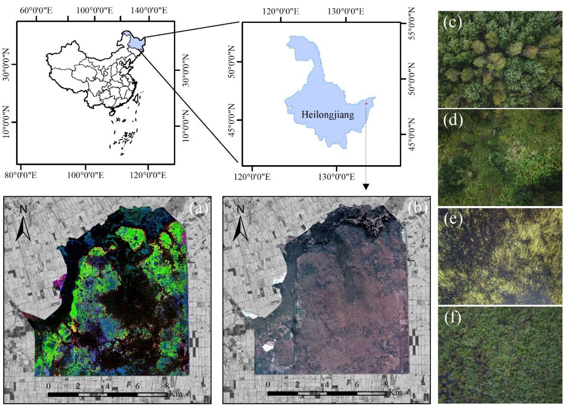
In this study, we used Honghe National Nature Reserve (HNNR) as the study area (Figure 1). HNNR is located at the junction of Tongjiang city and Fuyuan city in Heilongjiang Province, northeast of Sanjiang Plain, with an area of 21,835 hectares. The latitude and longitude ranges of the reserve are 133°34′38″–133°46′29″E and 47°42′18″–47°52′00″N, respectively, and it comprises a near-natural marsh ecosystem with a large variety of vegetation types, providing support for six endangered and rare species of flora and three of avifauna. The Nongjiang River and Wolulan River flow through the reserve and forms large areas of marshes [2]. HNNR has a typical warm temperate monsoon climate; annual rainfall is 585 mm, 50–70% precipitation is concentrated between July and September, and the annual freezing periods are about seven months. The reserve is mainly composed of forests, marshes, and open water, constituting a complete wetland ecosystem. The main vegetation types of the study area include White birch and poplar forest, Salix brachypoda, Carex lasiocarpa, Carex pseudo-curaica, and other herbaceous marsh vegetation. HNNR was listed as an important international wetland in 2002 and designated as one of the 36 internationally important wetlands in China. HNNR is the epitome of original marsh, which can fully reflect the overview of the original marsh in the Sanjiang Plain. Marsh vegetation mapping is a crucial step in carrying out wetland protection and sustainable development of HNNR.
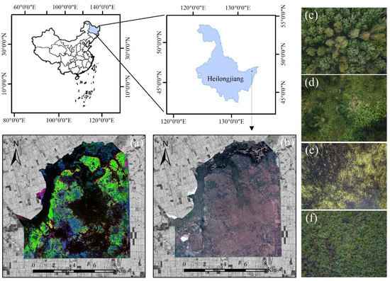
Figure 1.
The geographical location of the study area. (a) False-color composite image of ALOS-2 based on Freeman2 polarimetric decomposition; (b) true-color image of ZH-1 hyperspectral satellite; (c) forest; (d) shrub; (e) deep-water marsh vegetation; and (f) shallow-water marsh vegetation.
2.2. Data Source
2.2.1. Active and Passive Remote Sensing Images
This paper collected ZH-1 hyperspectral images, C-band GF-3, and L-band ALOS-2 quad-polarization SAR images for marsh vegetation mapping (Table 1). Zhuhai-1 (ZH-1) micro-satellite constellation is the main component of the “Satellite Spatial Information Platform” project of Zhuhai Orbit Control Engineering Co., Ltd. ZH-1 has achieved 12 satellites in orbit, which contains 8 hyperspectral satellites in a multi-orbit network operation. It is an important member of the global hyperspectral satellite family and the only commercial hyperspectral satellite constellation. ZH-1 hyperspectral images contain a total of 32 spectral bands with a spatial resolution of 10 m. Gaofen-3 (GF-3) is the first civilian C-band polarimetric SAR (synthetic aperture radar) imaging satellite of the CNSA (China National Space Administration), Beijing, China, which has 12 imaging modes with dual- and quad-polarization measurements. This study selected GF-3 SAR images from the quad-polarization strip 1 (QPSI) imaging mode. ALOS-2 is a Japanese land-observing satellite, which launched in May 2014 and carries a 1.2 GHz (L-band) PALSAR-2 radar. ALOS-2 is currently the only high-resolution L-band SAR commercial satellite in orbit.

Table 1.
Summary of main parameters of active and passive remote sensing images.
2.2.2. Field Measurements and Image Preprocessing
The sample data in this paper mainly came from field measurements and visual interpretation of ultra-high spatial resolution UAV images. Field measurements were collected on 25 to 30 April 2015, 24 to 30 August 2019, and 12 to 19 July 2021, respectively. We used a hand-held GNSS RTK receiver with a centimeter-level positioning accuracy for recording the geographic locations of 1 m × 1 m sampling plots. Moreover, we used the DJI UAV Phantom 4 Pro V.2.0, equipped with a 1-inch 20-megapixel CMOS sensor to take aerial photos of the study area. The flight height was 30–50 m. The flight time was 10:00 a.m.–3:00 p.m. (UTC/GMT + 8:00) with good weather conditions. Finally, the sampling data with the total 900 sample points in this paper was divided into seven land cover types: water, paddy field, cropland, shrub, forest, deep-water marsh vegetation, and shallow-water marsh vegetation (Table 2). All samples were randomly divided into 70% for training and 30% for testing.

Table 2.
Summary of the classification system and the number of sample data.
This paper used ENVI 5.5 software (ITT Exelis Visual Information Solutions, USA) to carry out the preprocessing of the ZH-1 hyperspectral images, mainly including radiometric calibration, atmospheric correction, and orthorectification. Then, we used the SARScape 5.6 software (SARMAP, Switzerland) to calculate the backscattering coefficients of GF-3 and ALOS-2 SAR images after the processing of multi-looking, filtering, and geocoding. GF-3 and ALOS-2 SAR images were resampled to a 10 m spatial resolution. Finally, we used the PolSARpro_v6.0 software (University of Rennes 1, France) to extract the coherency matrix (T3), and implement geocoding, filtering, and polarization decomposition. In this study, we used 23 coherent and incoherent polarimetric SAR decomposition methods to extract 152 polarimetric parameters from C-band GF-3 and L-band ALOS-2 quad-polarization SAR images, respectively (Table A1 in Appendix A). The ground control points of the study area measured by a hand-held GNSS RTK receiver were used to implement georeferencing of the ZH-1, GF-3, and ALOS-2 SAR images with the georeferencing errors less than a pixel. In this paper, all remote sensing images were unified to the same projected coordinate system (WGS_1984_UTM_Zone_49N).
2.3. Methods
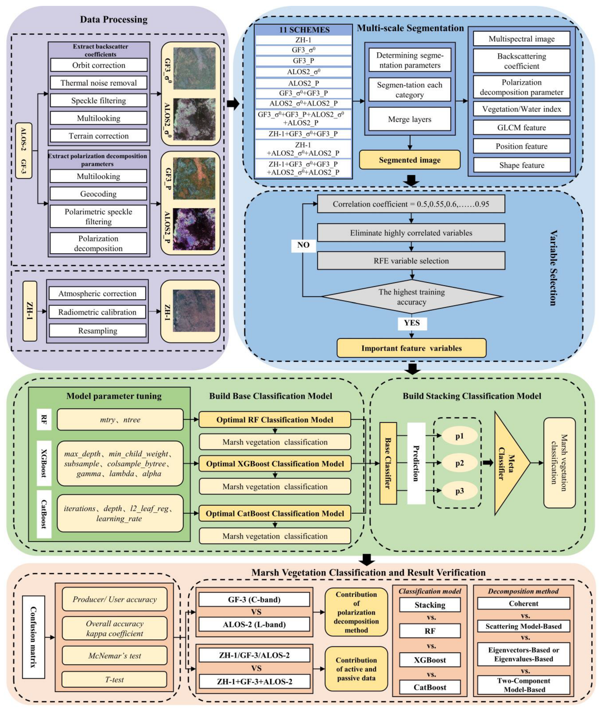
The workflow of this study includes three primary parts for marsh vegetation mapping (Figure 2). (1) We carried out the preprocessing of ZH-1 hyperspectral, GF-3, and ALOS-2 SAR images to obtain the spectral reflectance of original bands and backscatter coefficient, extracted multiple polarimetric parameters using four decomposition models, and constructed eleven classification schemes with different active and passive image combinations. (2) We performed iterative segmentation for each classification scheme, calculated the spectral indexes, texture, and position features, and constructed a multi-dimensional dataset of each scheme by combing different image features. Then, we used high-correlation elimination and recursive feature elimination (RFE) methods to reduce data redundancy and select the optimal input variables of each scheme. (3) This paper stacked Random Forest (RF), XGBoost, and CatBoost algorithms to build an ensemble learning classification model and implemented hyper-parameter tuning and model training. Finally, we examined the performance of the ensemble learning classification model using the hyperspectral and polarimetric SAR images, and demonstrated the feasibility of integrating hyperspectral and multi-wavelength polarimetric SAR images to improve the classification accuracy of marsh vegetation.
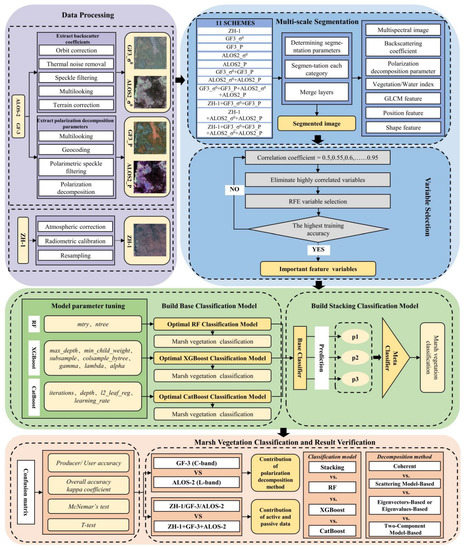
Figure 2.
Workflow of this study.
2.3.1. Image Segmentation and Construction of Classification Schemes
In this study, we used eCognition Developer 9.4 software (Trimble Geospatial, USA) to implement multi-scale inherited segmentation for ZH-1 hyperspectral, GF-3, and ALOS-2 SAR images. To segment marsh vegetation of HNNR with its most appropriate scale, we selected the optimal parameters combinations of segmentation scales, shape/color, and compactness/smoothness for each land cover type (Table 3). The final segmentation results of HNNR were derived from the fusion of segmentation of each optimal parameter combination. Then, we calculated the spectral indexes, texture, and position features (Table A2 in Appendix A) from the segmentation result of ZH-1 hyperspectral images. Finally, we combined the segmentation results of ZH-1 hyperspectral, GF-3, and ALOS-2 SAR images and constructed eleven classification schemes (Table 4). Each scheme has a multi-dimensional dataset with different image features.

Table 3.
Multi-scale segmentation parameters of different land cover types in the study area.

Table 4.
Classification Schemes with the combination of different feature variables from multi-sensor images.
2.3.2. Variable Selection and Construction of Marsh Vegetation Classification Model
In order to eliminate data redundancy and improve the efficiency and classification accuracy of models, we performed a variable selection from a multi-dimensional feature dataset for each scheme. In this paper, we used R Studio to eliminate high-correlation variables from the dataset in each scheme, where the correlation coefficients were set from 0.6 to 0.95 in steps of 0.05. After eliminating high correlation, further variable selection was conducted using the recursive feature elimination (RFE) method. According to the training accuracy of the RF model, we selected the optimal variables of each scheme to construct the marsh vegetation classification model. Table 5 shows the number of final variables and the training accuracy of the model.

Table 5.
The number of variables after high-correlation elimination and RFE-based variables selection, and the training accuracy of model.
Stacking is a hierarchical ensemble framework of embedding multiple base models that integrates the prediction results of each base classifier and uses the output values as training data for training the metamodel [34]. This study selected three ML classifiers (RF, XGBoost, CatBoost) as the base models and used the grid-search method for parameter tuning to find the optimal parameters for each model in different schemes. The specific tuning parameters of each classification model are shown in Table 6. This paper designed the stacking algorithm (Figure 3) with a two-step training process: (1) we used five-fold cross-validation to divide the training set after variable selection, and then input to RF, XGBoost, and CatBoost; (2) we selected the base model with the highest classification accuracy as the metamodel, and stacked the prediction results of the base models as the new training set and testing set. Finally, we used the new training set to train the metamodel for constructing an ensemble classification model of marsh vegetation.

Table 6.
Tuning parameters of classification models.
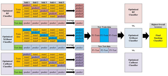
Figure 3.
The architecture of stacking ensemble learning-based classification model.
3. Results
3.1. Marsh Vegetation Classifications Using Hyperspectral and Quad-Polarization SAR Images
3.1.1. Quad-Polarization SAR Images with Different Frequencies
It can be seen from Table 7 that four classification models had excellent stability, and the standard error of overall accuracy was less than 3%. The schemes based on ALOS-2 SAR data (schemes 4, 5, and 7) achieved better classification accuracy with an average overall accuracy of over 85%, which was 6.56–12.56% higher than the GF-3 SAR data (schemes 2, 3, and 6). These results showed that the schemes with the ALOS-2 quad-polarization SAR images achieved better performance than the schemes with the GF-3 quad-polarization SAR images when using the same classification algorithm. Moreover, after integrating the backscattering coefficients and polarimetric parameters of GF-3 and ALOS-2 (scheme 8), the overall accuracy of the model improved by 3.86–7.30% compared to only using the backscattering coefficients or polarimetric parameters (scheme 6). However, the overall accuracy of scheme 8 decreased by 3.86–5.15% when compared to only using the backscattering coefficients or polarimetric parameters of ALOS-2 (scheme 7).

Table 7.
Overall accuracy and standard errors of the models in different classification schemes using C-band and L-band quad-polarization SAR images. OA, overall accuracy; AOA, average overall accuracy.
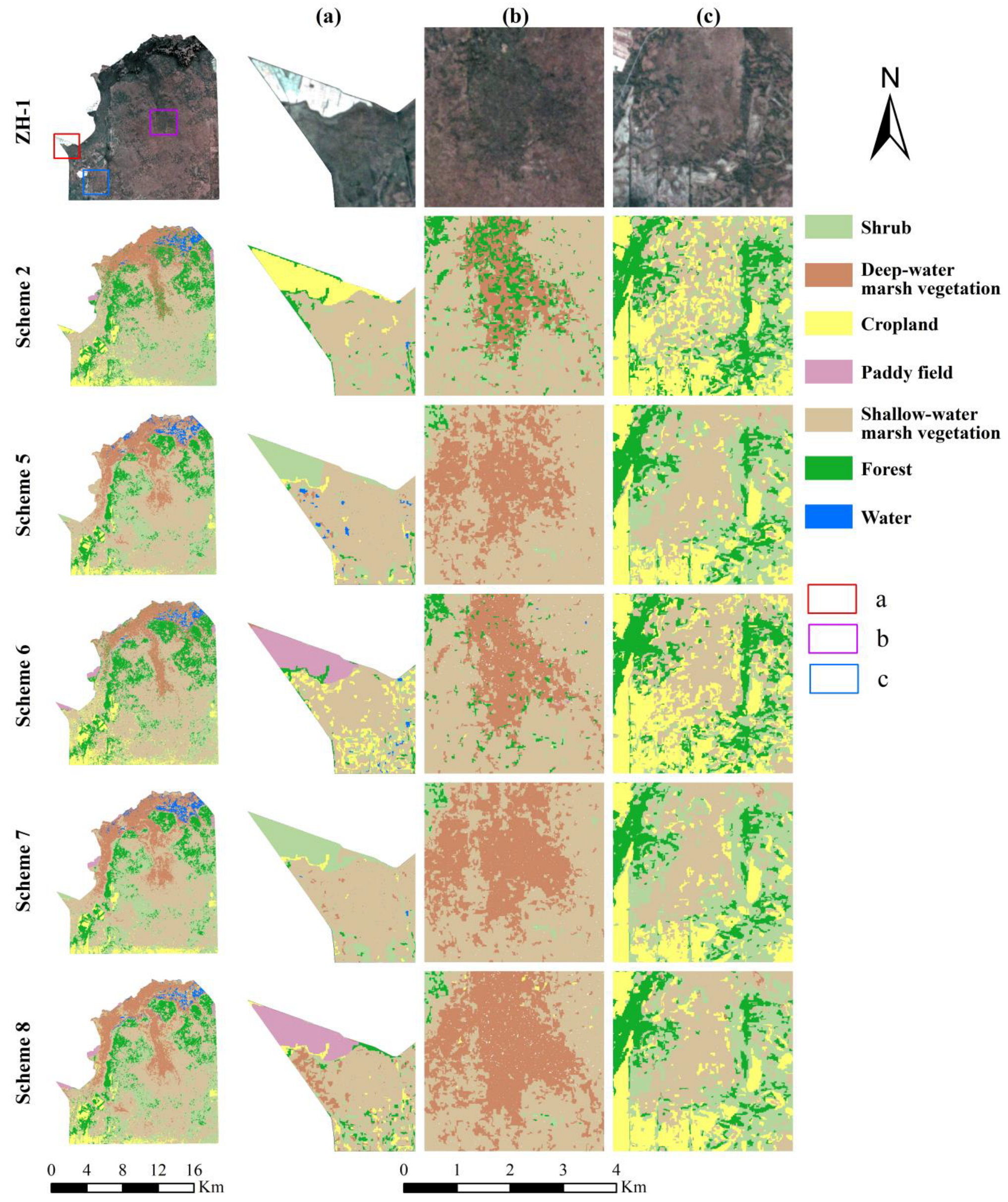
It can be seen from Figure 4 that scheme 2, only using the backscattering coefficient of GF-3, achieved poor classification results, especially with the serious confusion between forests and swamp vegetation, and between dryland and shallow-water swamp vegetation. Although the classification result of scheme 5, based on the polarimetric parameters of ALOS-2, was better than scheme 2, it still could not effectively distinguish deep-water marsh vegetation, shallow-water marsh vegetation, and shrubs. Schemes 6 and 7 had higher classification results than schemes 2 and 5, which indicated that integrated backscattering coefficients and polarimetric parameters could improve the accuracy. Although the classification accuracy of scheme 8, by integrating GF-3 and ALOS-2, was lower than scheme 5 and scheme 7, it was more effective in distinguishing between paddy fields and shrubs. For example, the paddy field in Figure 4a was correctly classified by schemes 6 and 8, while it was misclassified as other vegetation types in the other schemes. In Figure 4b, forest and deep-water marsh vegetation could be accurately identified by schemes 5, 7, and 8 while they were mixed with each other in schemes 2 and 6. Moreover, schemes 2 and 6 could not clearly distinguish cropland from shallow-water marsh vegetation (Figure 4c), but schemes 5 and 7 could resolve this problem.
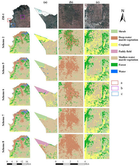
Figure 4.
Classification results of different schemes using the optimal models. (a) Paddy filed; (b) Deep-water marsh vegetation; (c) Shallow-water marsh vegetation and cropland.
3.1.2. Integrating Hyperspectral and the Quad-Polarization SAR Images
As can be seen from Table 8, scheme 11 achieved the highest classification accuracy with an average overall accuracy of 92.38%, which was 7.83% and 1.61% higher than schemes 9 and 10, respectively. Moreover, scheme 11 improved the overall accuracy of each model from 5.58% to 9.01% compared to scheme 8 only integrating GF-3 and ALOS-2. The CatBoost model achieved the highest overall accuracy of 79.57% when only using hyperspectral data. After adding quad-polarization SAR data, the classification accuracies of four classification models were consistently improved. The overall accuracy of schemes 9 and 10 was 5.80–15.25% higher than scheme 1. In addition, scheme 9 increased the overall accuracy of each classification model from 3.00% to 7.30% compared with scheme 6. The overall accuracy of all models built by scheme 10 was higher than scheme 7, except for XGBoost, which indicated that integrating hyperspectral and quad-polarization SAR images could effectively improve the performance for classifying marsh vegetation. Integrating L-band polarimetric SAR data with hyperspectral images could achieve higher overall accuracy in the same scheme of integrating active and passive remote sensing images. The average overall accuracy of scheme 10 was raised by 6.22% compared with scheme 9, and the overall accuracy of each classification model was improved by 4.72–8.16%.

Table 8.
Overall accuracy and standard errors of each classification model by integrating hyperspectral and quad-polarization SAR images. OA, overall accuracy; AOA, average overall accuracy.
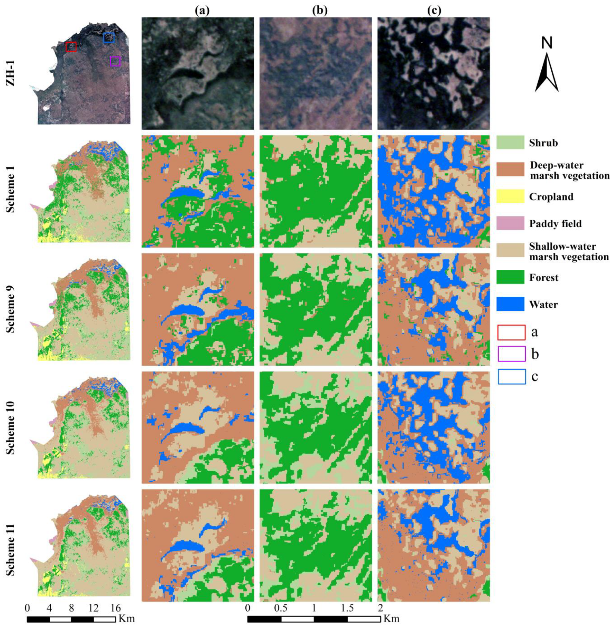
As shown in Figure 5, scheme 1 using ZH-1 hyperspectral images produced unsatisfactory classifications with large-scale confusion between cropland and aquatic plants, and between water and deep-water marsh vegetation. The classification results of schemes 9, 10, and 11 that integrated hyperspectral and polarimetric SAR images were better than the scheme only using a single data source. Scheme 11, which integrated ZH-1, GF-3, and ALOS-2 multi-source images, produced the optimal classifications that were consistent with the distribution of ground objects. As shown in Figure 5a, shallow-water and deep-water marsh vegetation in different areas were misclassified as forest in schemes 1 and 9, and there was a small amount of confusion between deep-water marsh vegetation and water body in scheme 10. Forest and shrubs were more accurate and detailed identification in schemes 10 and 11 (Figure 5a,b). In Figure 5c, scheme 1 misclassified the large area of deep-water marsh vegetation into water. Nevertheless, schemes 9 and 10, which combined hyperspectral with quad-polarization SAR images, reduced their misclassification area. The above results indicate that integrating hyperspectral images and quad-polarization SAR data is helpful for classifying submerged deep-water marsh vegetation, especially when adding GF-3 images.
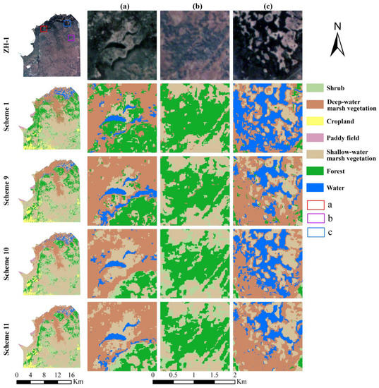
Figure 5.
Classification results of integrating hyperspectral and quad-polarization SAR images using the optimal classifiers. (a) Water, deep-water and shallow-water marsh vegetation; (b) Forest and shrub; (c) Water and deep-water marsh vegetation.
3.1.3. Statistical Analysis of the Classification Performance of Each Scheme
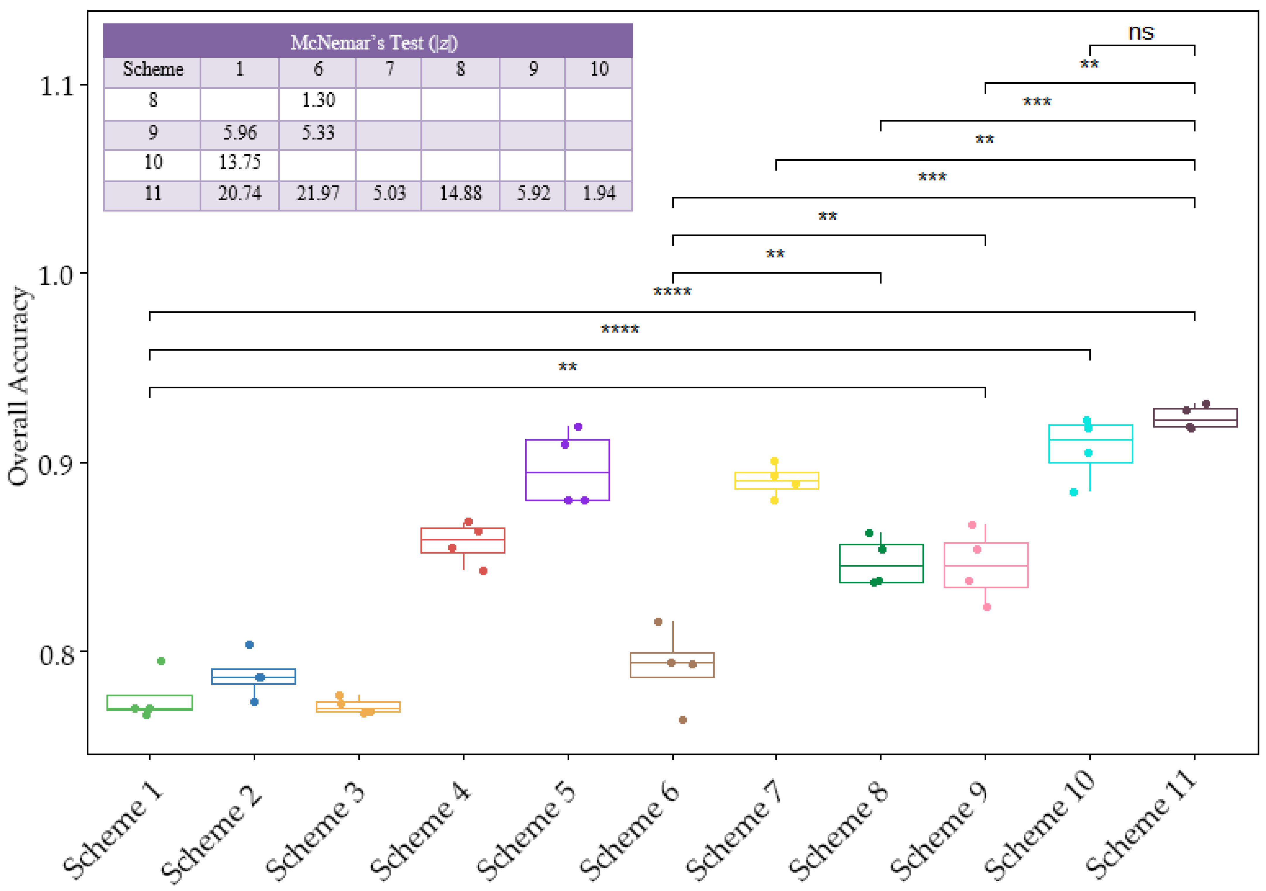
From the overall distribution of the boxplot in Figure 6, we found that schemes 1, 2, and 3 could not obtain high classification accuracy using the single hyperspectral or SAR image. The overall accuracy of L-band ALOS-2 images (schemes 4, 5, 7, and 10) was higher than C-band GF-3 data (schemes 2, 3, 6, and 9). Scheme 9 or 10, which integrated hyperspectral images and quad-polarization SAR images, significantly improved overall accuracy compared to only using a single data source. In this paper, the t-test and McNemar test were performed for the classification of the accuracy of eleven schemes [39,40] and further used to clarify the significant difference in classification schemes. In Figure 6, we found there were significant differences between schemes 9, 10, and 11 and scheme 1 based on the t-test and the McNemar test. These results demonstrated that combining quad-polarization SAR images with hyperspectral data could significantly improve the classification accuracy of marsh vegetation. The significant differences between schemes 6, and 9, 11 indicated adding ZH-1 and ALOS-2 images influenced the classification performance of GF-3 SAR sensor for wetland vegetation mapping. The classification results between schemes 6 and 8 without significant differences indicated that the combination of C-band GF-3 and L-band ALOS-2 could not improve the classification accuracy of marsh vegetation. The t-test between schemes 6 and 8, 9 showed significant differences, and the |z| value of the McNemar test between schemes 6 and 11 reached 21.97, which indicated that adding ZH-1 and ALOS-2 images could significantly improve the classification accuracy based on GF-3 data. There were very significant differences between schemes 8 and 11, indicating that ZH-1 hyperspectral images were also an important variable for marsh vegetation mapping.
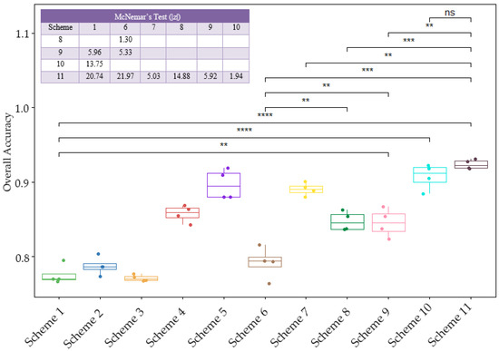
Figure 6.
Statistical boxplots of overall accuracy for eleven classification schemes using four models. Different number of ‘*’ represents the significant difference of classification schemes at different confidence levels in the t-test. ns: p > 0.05**: p ≤ 0.01; ***: p ≤ 0.001; ****: p ≤ 0.0001. McNemar test: the difference in classification results was significant at the 95% confidence level when |z| > 1.96.
This paper analyzed classification accuracy improvement of marsh vegetation when kinds of variables are introduced by multi-source sensors (Table 9). we found that a combination of hyperspectral, C-band, and L-band SAR images improved the average classification accuracy of each vegetation type from 3.81% to 19.70%, which indicated that SAR images could enhance the spectral separability of marsh vegetation. The hyperspectral variables introduced SAR images that significantly improved the average accuracy (more than 15%) of deep-water and shallow-water marsh vegetation. Integration of the C-band backscatter coefficient and polarization decomposition parameters improved by 7.51% the average accuracy of shrub when compared to that using the polarization parameters, so backscatter coefficient was an important variable for identifying shrubs. The average accuracy of shrub and deep-water marsh vegetation improved by 16.24% and 6.76% from scheme 6 to scheme 8, respectively, indicating that the L-band with the longer wavelength was more capable of distinguishing vegetation with a dense canopy and identifying aquatic plants.

Table 9.
Improvement of average accuracy (half of the user accuracy and producer accuracy) for different marsh vegetation when kinds of variables introduced by multi-source sensors.
3.2. Effect of Different Classification Models on Marsh Vegetation Mapping
3.2.1. Stacking Ensemble Learning for Marsh Classification
Figure 7 displays the range of overall accuracy of four classification models. XGBoost and the Stacking model both achieved better average overall accuracy for all schemes and reached 85.44% and 85.09%, respectively. The average overall accuracy of Stacking was 1.25% and 1.44% higher thsn the RF and XGBoost models, respectively. A comparison of the range (box) of overall accuracy derived from four classification models found that Stacking was more sensitive to data combinations and had a wide range of variation in classification accuracy. According to the length of the error bar, we found that Stacking was more stable for mapping marsh vegetation than other models in eleven schemes, while XGBoost displayed a relatively large fluctuation range. From the distribution of the scatter points, we found that there were more schemes that achieved over 85% overall classification accuracy when using Stacking, which indicated that Stacking could improve the classification accuracy of marsh vegetation using active and passive data combinations (scheme 5, 7, 10 and 11). Scheme 10 used Stacking and reached 92.27% of overall classification accuracy, the highest accuracy of all classification models.
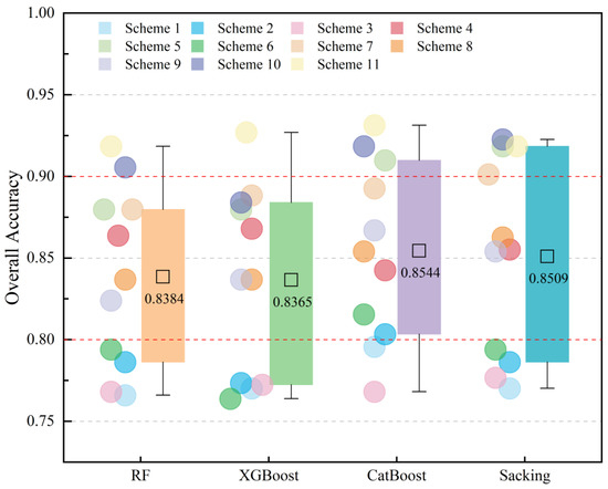
Figure 7.
Overall accuracy distribution of all schemes based on four classification models.
3.2.2. Comparison of the Performance of Classification Models for Different Vegetation Types
This paper used the average accuracy as a metric to evaluate the effectiveness of the classification model for identifying different marsh vegetation (Figure 8). The forest obtained the highest average accuracy and produced the most stable classification, in which the mean value of average accuracy reached 92.1% based on the CatBoost model. Deep-water marsh vegetation was identified by the CatBoost model, with an average accuracy of 80.4%. Shallow-water marsh vegetation and shrub achieved the highest average accuracy (84.8% and 80.2%) using the Stacking model, respectively. The classification stability of shallow-water marsh vegetation was higher than deep-water marsh vegetation, especially when using XGBoost, CatBoost, and Stacking classification models. The average classification accuracy of shrubs was the least stable and varied widely in all schemes.
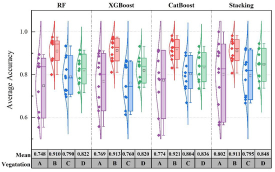
Figure 8.
Distribution of the average accuracy of each vegetation type using four classification models with all schemes. A, shrub; B, forest; C, deep-water marsh vegetation; D, shallow-water marsh vegetation.
3.3. Influence of Hyperspectral Image Features and Polarimetric Decomposition Parameters on Marsh Vegetation Classification
3.3.1. Evaluation of Contribution of Hyperspectral Image Features and Polarimetric Decomposition Parameters to Classify Marsh Vegetation
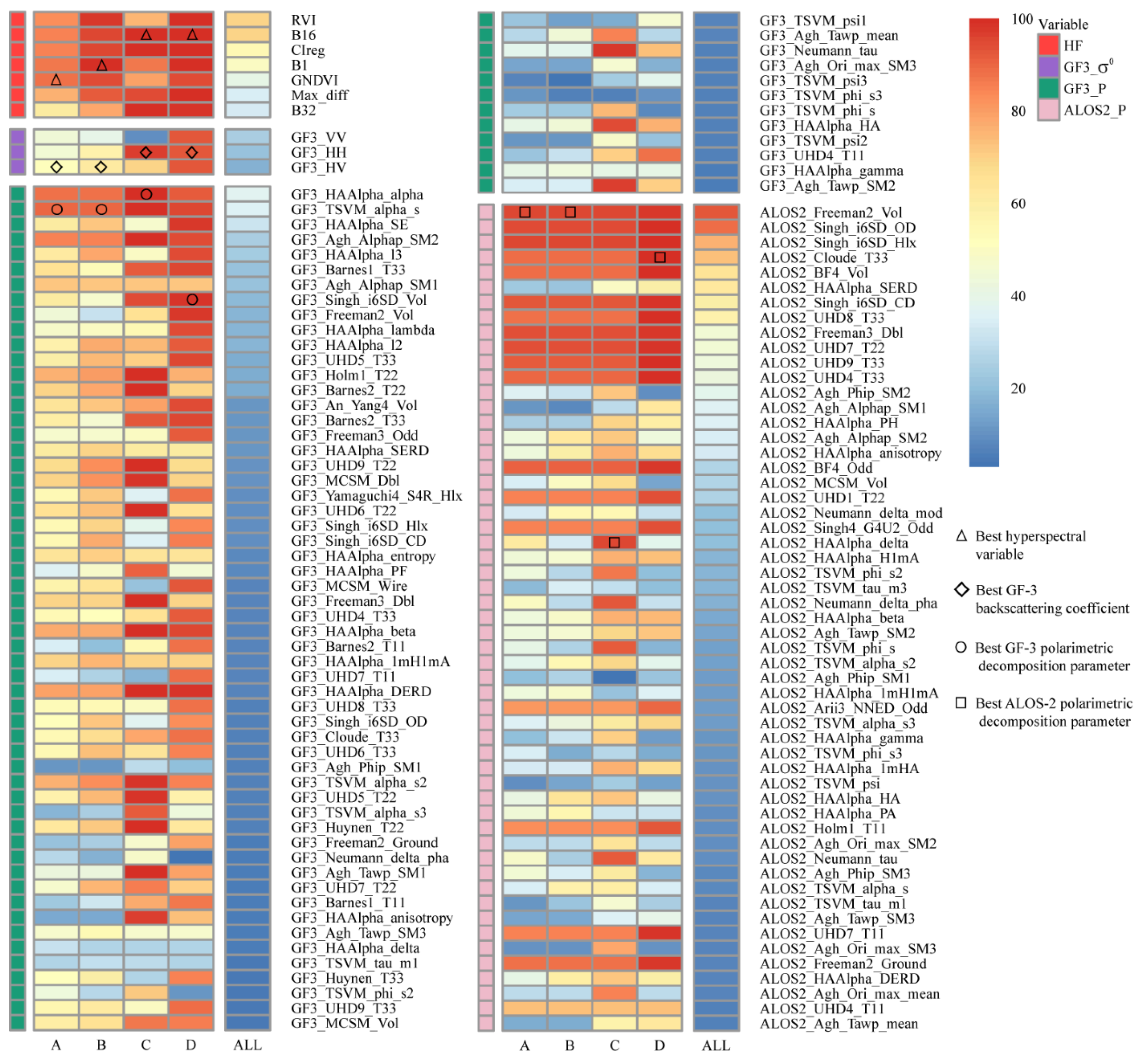
Figure 9 shows the contribution of feature variables from hyperspectral and quad-polarization SAR images to classify marsh vegetation. The importance scores of variables were counted based on the data sources, and Table 10 shows the proportion of the contribution of active and passive features to marsh vegetation classification. Hyperspectral bands (B1 and B16) and GNDVI were highly important for classifying deep-water and shallow-water marsh vegetation. Within the C-band backscattering coefficients, GF3_HV is better at identifying shrubs and forests, and GF3_HH was the critical variable for the classification of shallow-water and deep-water marsh vegetation. GF-3_TSVM_alpha_s and ALOS2_Freeman2_Vol were the best C-band and L-band polarization decomposition parameters for classifying shrubs and forests, respectively. From the proportion of the contribution of active and passive remote sensing data, Hyperspectral features were most useful for forest classification. ALOS-2 with the longer wavelength played an essential role in distinguishing deep-water marsh vegetation, with a 42% contribution of ALOS-2 polarization parameters. The shorter wavelength GF-3 was most suitable for classifying shallow-water marsh vegetation, and its backscattering coefficient and polarimetric parameters accounted for the highest proportion of contribution in all vegetation types.
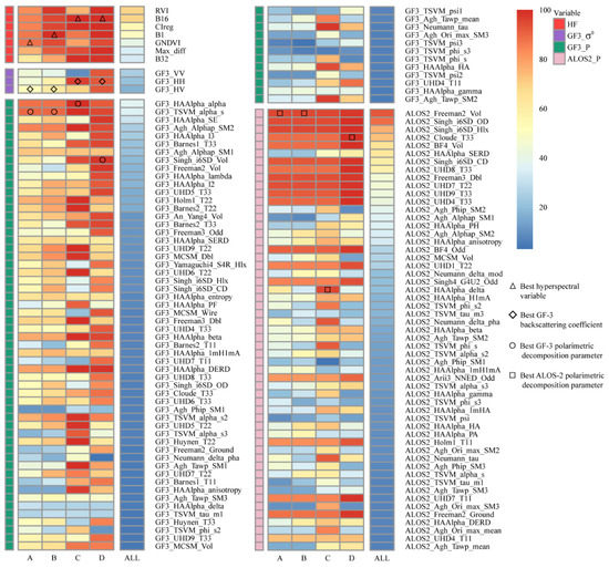
Figure 9.
Contribution of feature variables to classify marsh vegetation derived from hyperspectral and quad-polarization SAR images. A, shrub; B, forest; C, deep-water marsh vegetation; D, shallow-water marsh vegetation. HF, hyperspectral Features.

Table 10.
Summary of the proportion of the contribution of active and passive features to marsh vegetation classification.
3.3.2. Influence of Polarimetric SAR Decomposition Methods on Marsh Vegetation Classification
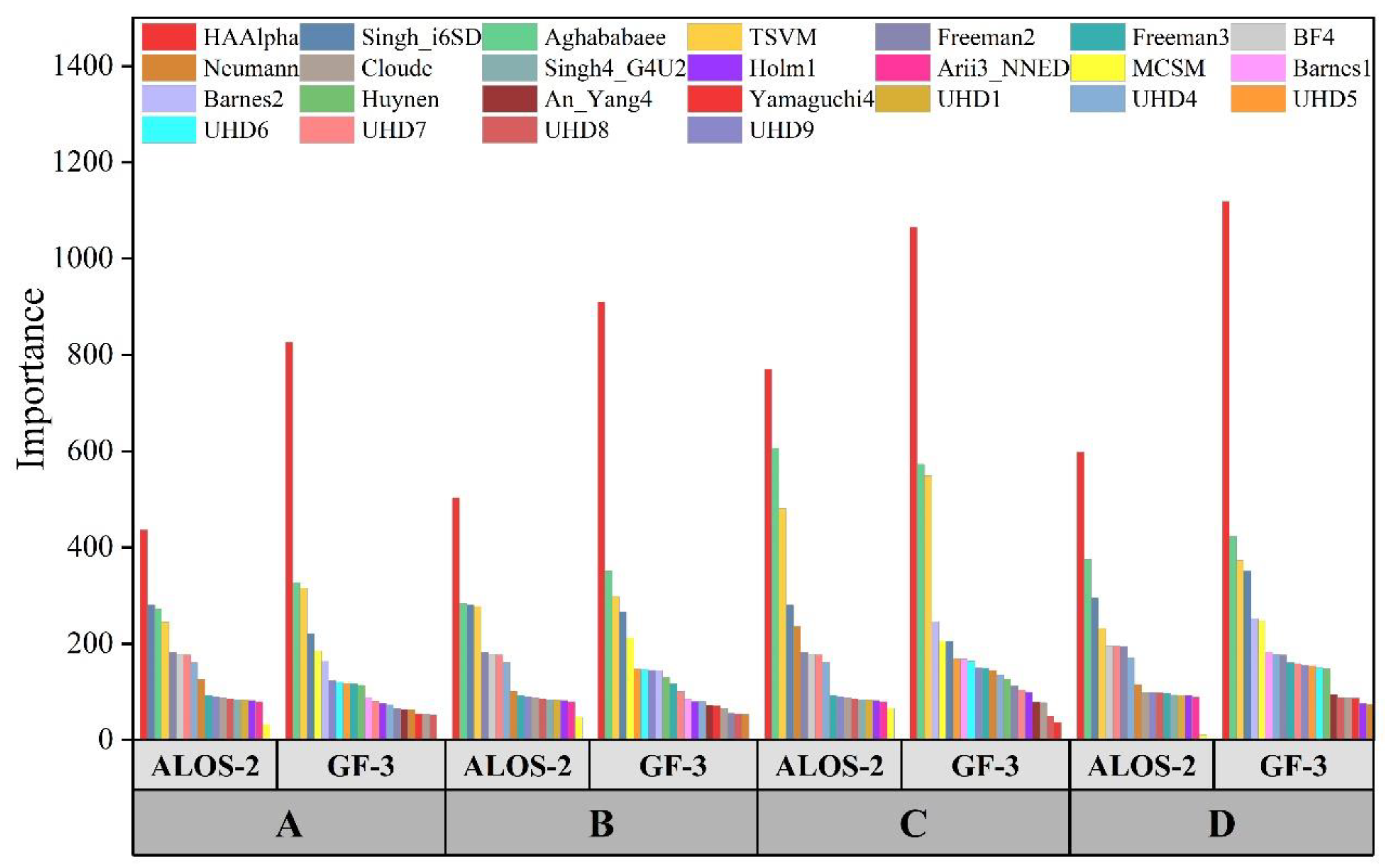
In this study, the polarimetric parameters obtained from the GF-3 and ALOS-2 quad-polarization SAR data using different decomposition methods were used to make a statistical analysis of the importance of the marsh vegetation classification. It can be seen from Figure 10 that the HA-Alpha decomposition method was the optimal one for classifying marsh vegetation when using GF-3 and ALOS-2 quad-polarization SAR data, followed by the Agh decomposition method. Furthermore, for GF-3, the TSVM and Singh i6SD decomposition methods outperformed others for the differentiation of shrub, forest, and shallow-water marsh vegetation, while the decomposition method Barnes2 based on coherent-based two components had higher importance than the decomposition method Singh i6SD for deep-water marsh vegetation. For ALOS-2, TSVM, and Singh i6SD decomposition methods contributed significantly to identifying each marsh vegetation. The Singh i6SD decomposition method ranked second in the sensitivity to shrub classification, and the Agh decomposition method ranked second in importance for classifying forests, deep-water marsh vegetation, and shallow-water marsh vegetation.
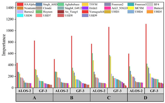
Figure 10.
Contribution of polarimetric parameters of GF-3 and ALOS-2 to marsh vegetation classification using different decomposition methods. A, shrub; B, forest; C, deep-water marsh vegetation; D, shallow-water marsh vegetation.
As can be seen from Figure 11, when using ALOS-2 data, the multiple-components scattering mechanism model provided more contribution to identify marsh vegetation than other models and was the most important for the identification of shrubs, with a contribution of 36%. The proportion of the contribution of the coherent target decomposition was the largest for deep-water marsh vegetation, while that of the coherent-based two components was the least. The eigenvector/eigenvalue of the scattering matrix had the highest percentage contribution of all vegetation types in identifying deep-water marshes and shallow-water marshes, accounting for 25%. When using GF-3 to classify marsh vegetation, the eigenvector/eigenvalue of the scattering matrix provided the most important contribution to identifying shrubs and forests, which was the opposite of using ALOS-2. The importance of coherent target decomposition for deep-water marsh vegetation using the C-band GF-3 SAR images was similar to L-band ALOS-2. The multiple-components scattering mechanism model was of the smallest importance in the four decomposition models. Moreover, the coherent-based two-component and multiple-component scattering mechanism models were most useful for the classification of shallow-water marsh vegetation. Whether using GF-3 or ALOS-2, the proportion of the contribution of coherent target decomposition to the classification of marsh vegetation was the least compared to the other three incoherent decomposition methods.
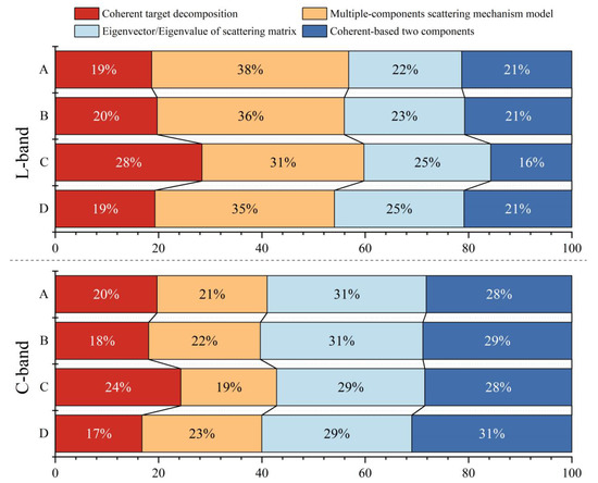
Figure 11.
Contribution of polarimetric parameters to marsh vegetation classification using four polarimetric decomposition methods. A, shrub, B, forest, C, deep-water marsh vegetation, D, shallow-water marsh vegetation.
4. Discussion
In this study, integrating hyperspectral and quad-polarization SAR data (schemes 9, 10, and 11) acquired better classification results than only using single data, and the confusion of forests, shrubs, and herbaceous vegetation was clearly reduced. These results indicated that integrating hyperspectral and quad-polarization SAR data can effectively improve the classification accuracy of marsh vegetation [41]. This was because optical images acquired the spectral reflection characteristics of the object’s surface. However, such characteristics might be similar for different vegetation, making it difficult to classify them using optical imagery [42,43]. In contrast, SAR images can penetrate vegetation to obtain information below the vegetation canopy, so the SAR feature improved the separability of this spectrally-similar vegetation [44,45]. Moreover, combining hyperspectral and ALOS-2 images for wetland classification produced some misclassifications between deep-water marsh vegetation and water, but the classification model decreased the confusion between them when adding C-band GF-3 quad-polarization SAR data. Therefore, integrating the polarimetric SAR data of different frequencies can take full advantage of each SAR sensor to reduce category confusion and improve classification accuracy. Nevertheless, we also found that only integrating the different frequencies quad-polarization SAR data cannot always produce the optimal classification results between schemes 4, 5, 6, and scheme 8 with 3.86% to 5.15% differences. The overall accuracy of marsh vegetation reached 93.13% using integrating ZH-1 hyperspectral, GF-3, and ALOS-2 images, which demonstrated that the additional hyperspectral images could effectively improve the capability and stability of wetland classification. These results demonstrated that ZH-1 hyperspectral images provided a great performance for marsh vegetation mapping. Therefore, the combination of hyperspectral images and quad-polarization SAR data could realize the high-precision mapping of marsh vegetation and provide data support for the restoration and conservation of marshland ecosystems.
RF has the advantages of high classification accuracy and less overfitting under high-dimensional datasets [46]. XGBoost controls the complexity of the model by adding a regularization term [47]. Catboost uses ranking boosting to handle noisy points in the training set, thus avoiding gradient and prediction bias [48]. These three algorithms provide over 76% overall accuracy for eleven classification schemes in this paper. Stacking built by integrating the above three algorithms achieved an effective identification of wetlands with complex land cover types [49,50], with the highest OA of 92.27%. The classification accuracy of shrubs was low and showed instability, which was easily affected by the combination of data sources. Stacking produced the best classifications of shrubs and shallow-water marsh vegetation, and improved the classification accuracy of shrubs, resulting in increasing the overall accuracy of marsh vegetation in the HNNR. The rhizomes of shallow-water marsh vegetation are submerged in water, and the scattering mechanism is similar to that of paddy fields [51]. Therefore, Stacking has a better identification and classification results on shallow-water marsh vegetation. In the single classification model, the CatBoost algorithm produced the best classification performance and achieved the highest classification accuracies of forests and deep-water marsh vegetation. Previous studies reported that CatBoost improved classification accuracy and stability and decreased computational cost compared to the traditional decision-tree algorithm [52]. Luo et al. [53] found that CatBoost significantly improved the classification accuracy compared to the RF and XGBoost models. Understanding the advantages of different classifiers for vegetation recognition could improve the accuracy of vegetation mapping, which is conducive to researching the differences between carbon sinks in different geographic environments to achieve global sustainable development and protect carbon sinks [54,55].
The overall classification accuracy of the schemes based on L-band ALOS-2 quad-polarization SAR data is higher than that using C-band GF-3 quad-polarization SAR data. On the one hand, it is because the spatial resolution of ALOS-2 is higher than that of GF-3. On the other hand, the L-band with a longer wavelength is more penetrating than C-band, and has less attenuation when penetrating the vegetation canopy [56]. However, we found that the additional C-band polarimetric SAR data (scheme 8) could effectively reduce the confusion of paddy fields, croplands, and shrubs. Therefore, for accurate identification of different vegetation types, L-band ALOS-2, and C-band GF-3 quad-polarization SAR data should be reasonably selected. In the study, the L-band has better recognition of shrubs than the C-band. The reason for this may be that long waves have stronger penetration than short waves and can obtain ground-backscattered echoes attenuated by the canopy [57], increasing the difference between shrubs and other features. Using L-band, more energy could penetrate the canopy of deep-water marsh vegetation. Therefore, volume scattering and canopy attenuation will be the predominant interactions and higher returned signal compared to C-band. C-band is more advantageous in recognizing semi-submerged shallow-water marsh vegetation and paddy field. This type of vegetation height is low in height and densely distributed, and the water body enhances the volume scattering interaction between C-Band and this plant [58]. Studies have shown that short-wavelength SAR images have better identification results for herbaceous marsh vegetation and water under short vegetation [59,60,61,62]. In addition, several studies have confirmed that the C-band backscattering coefficient has a powerful capability of discriminating treed and non-treed wetlands [63,64].
The traditional polarimetric decomposition methods HA-Alpha and TSVM proved to be effective for wetland classification [44,65], but the emerging polarimetric decomposition methods Singh_i6SD and Aghababaee also showed great potential. It shows that the introduction of a multi-type polarimetric decomposition method is effective in increasing the classification accuracy of marsh vegetation. As mentioned by Shimoni et al. [66], different polarimetric decomposition methods should all be applied in land cover classification, as they emphasize different land types. The contribution of the coherent polarimetric decomposition method to marsh vegetation classification is lower than that of the three incoherent polarimetric decomposition methods. This is because the ground objects in wetlands are distributed targets, and incoherent decomposition can better characterize them [67]. When using ALOS-2, the scattering mechanism model contributes more to various marsh vegetation than other decomposition models, especially the contribution to shrubs is the highest among all vegetation. The primary scattering mechanism of shrubs is volume scattering, and the decomposition method based on the scattering mechanism model is advantageous for vegetation, with volume scattering as the dominant scattering mechanism [44]. When using GF-3 images, the contribution of the coherent-based two components to shallow-water marsh vegetation is the highest among all vegetation, which plays an important role in distinguishing shallow-water marsh vegetation from deep-water marsh vegetation. Therefore, the combination of different polarimetric SAR decomposition methods and polarimetric SAR data in different frequency bands is demanded for improving the ability of marsh vegetation classification in the future.
5. Conclusions
In this study, we integrated backscattering coefficient and polarimetric decomposition parameters of C-band and L-band quad-polarization SAR data with ZH-1 hyperspectral images to classify marsh vegetation in the HNNR, northeast China using a stacking ensemble learning algorithm. We found that the additional hyperspectral images improved the performance of quad-polarization SAR data for mapping marsh vegetation, and integration of ZH-1 hyperspectral, C-band GF-3, and L-band ALOS-2 images obtained the highest overall accuracy (93.13%). This paper confirmed that ALOS-2 polarimetric SAR data outperformed GF-3 images in marsh vegetation classification, and further found that ALOS-2 was sensitive to identifying deep-water marsh vegetation, while GF-3 was sensitive to classify shallow-water marsh vegetation due to penetration of radar wavelength. We examined the applicability and generalization of stacking ensemble learning to classify marsh vegetation in different schemes using multi-source data, and proved that stacking ensemble learning provided good performance for mapping marsh vegetation and achieved 92.27% overall classification accuracy, which is better than that of a single machine-learning classifier. We revealed that the incoherent polarimetric decomposition method can better display the scattering mechanism of marsh vegetation when compared to the coherent polarimetric decomposition. The polarimetric parameters of ALOS-2 SAR images produced by scattering model-based decomposition method provided more contributions to distinguish various different types of marsh vegetation types. While eigenvector or eigenvalue-based and two-component polarimetric decomposition methods were more suitable when using GF-3 data. These results provide a scientific foundation for marsh preservation and restoration.
Author Contributions
Conceptualization, H.Y. and B.F.; methodology, H.Y. and S.X.; software, S.X. and D.F.; validation, Y.Z. and E.G.; formal analysis, H.Y.; investigation, S.L.; resources, Y.Z.; data curation, J.Q. and S.L.; writing—original draft preparation, H.Y. and S.X.; writing—review and editing, B.F.; visualization, H.Y.; supervision, D.F.; project administration, B.F.; funding acquisition, B.F. All authors have read and agreed to the published version of the manuscript.
Funding
This work was supported by the Guangxi Science and Technology Program (Grant number GuikeAD20159037), the Innovation Project of Guangxi Graduate Education (Grant number YCSW2022328), the National Natural Science Foundation of China (Grant number 41801071), the Natural Science Foundation of Guangxi Province (CN) (Grant number 2018GXNSFBA281015), and the “BaGui Scholars” program of the provincial government of Guangxi, the Guilin University of Technology Foundation (Grant number GUTQDJJ2017096). We appreciate the anonymous reviewers for their comments and suggestions, which helped to improve the quality of this manuscript.
Data Availability Statement
Not applicable.
Conflicts of Interest
The authors declare no conflict of interest.
Appendix A

Table A1.
Summary of polarimetric decomposition methods and polarimetric parameters used in this paper.
Table A1.
Summary of polarimetric decomposition methods and polarimetric parameters used in this paper.
| Decomposition Models | Methods | Parameters |
|---|---|---|
| Coherent target decomposition | Touzi (TSVM) | Twenty parameters including TSVM_alpha_s1, TSVM_alpha_s2, TSVM_alpha_s3, etc. |
| Aghababaee (Agh) | Agh_Alphap_SM1, Agh_Alphap_SM2, Agh_Alphap_SM3 etc. 19 parameters | |
| Coherent-based two components | Huynen | Huynen_T11, Huynen_T22, Huynen_T33 |
| Barnes 1 | Barnes1_T11, Barnes1_T22, Barnes1_T33 | |
| Barnes 2 | Barnes2_T11, Barnes2_T22, Barnes2_T33 | |
| UHDx (UHD1-9) | UHDx_T11, UHDx_T22, UHDx_T33 | |
| Multiple-components scattering mechanism model | Freeman two components (Freeman2) | Freeman2_Vol, Freeman2_Ground |
| Freeman three components (Freeman3) | Freeman3_Dbl, Freeman3_Odd, Freeman3_Vol | |
| Yamaguchi three components (Yamaguchi3) | Yamaguchi3_Dbl, Yanaguchi3_Odd, Yamaguchi3_Vol | |
| Yamaguchi four components (Yamaguchi4) | Yamaguchi4_S4R_Dbl, Yamaguchi4_S4R_Hlx, Yamaguchi4_S4R_Odd, Yamaguchi4_S4R_Vol | |
| Bhattacharya&Frery four components (BF4) | BF4_Dbl, BF4_Hlx, BF4_Odd, BF4_Vol | |
| Neumann two components (Neumann) | Neumann_delta_mod, Neumann_delta_pha, Neumann_tau | |
| Arii three components (Arii3_NNED) | Arii3_NNED_Dbl, Arii3_NNED_Odd, Arii3_NNED_Vol | |
| Singh four components (Singh_G4U2) | Singh4_G4U2_Dbl, Singh4_G4U2_Hlx, Singh4_G4U2_Odd, Singh4_G4U2_Vol | |
| L.Zhang five components (MCSM) | MCSM_Dbl, MCSM_Hlx, MCSM_DblHlx, MCSM_Odd, MCSM_Vol, MCSM_Wire | |
| Singh-Yamaguchi six components (Singh_i6SD) | Singh_i6SD_CD, Singh_i6SD_Dbl, Singh_i6SD_Hlx, Singh_i6SD_OD, Singh_i6SD_Odd, Singh_i6SD_Vol | |
| Eigenvector /Eigenvalue of scattering matrix | HA-Alpha decomposition (HA-Alpha) | HA-Alpha_T11, HA-Alpha_T22, HA-Alpha_T33, etc. |
| Cloude-Pottier (Cloude) | Cloude_T11, Cloude_T22, Cloude_T33 | |
| Holm 1 | Holm1_T11, Holm1_T22, Holm1_T33 | |
| Holm 2 | Holm2_T11, Holm2_T22, Holm2_T33 | |
| An &Yang three components (An_Yang3) | An_Yang3_Dbl, An_Yang3_Odd, An_Yang3_Vol | |
| An &Yang four components (An_Yang4) | An_Yang4_Dbl, An_Yang4_Hlx, An_Yang4_Odd, An_Yang4_Vol | |
| Van Zyl (1992) three components (VanZyl3) | VanZyl3_Dbl, VanZyl3_Odd, VanZyl3_Vol |

Table A2.
Description of the multi-dimensional dataset.
Table A2.
Description of the multi-dimensional dataset.
| Features | Description |
|---|---|
| Spectral bands | Thirty-two spectral bands, Brightness, Max. diff |
| Texture and position Features | GLCM_Homogeneity, GLCM_Contrast, GLCM_Dissimilarity, GLCM_Entropy, GLCM_An.2nd_moment, GLCM_Mean, GLCM_Correlation, GLCM_StdDev, Distance, Coordinate |
| Spectral indexes | CIgreen, CIreg, NDVI, RVI, GNDVI, NDWI |
| Backscatter Coefficient (σ0) | σ0VV, σ0VH, σ0HH, σ0HV |
| Polarimetric parameters | Shown in Table A1 |
References
- Hu, S.; Niu, Z.; Chen, Y.; Li, L.; Zhang, H. Global wetlands: Potential distribution, wetland loss, and status. Sci. Total Environ. 2017, 586, 319–327. [Google Scholar] [CrossRef] [PubMed]
- Zhou, D.; Gong, H.; Wang, Y.; Khan, S.; Zhao, K. Driving Forces for the Marsh Wetland Degradation in the Honghe National Nature Reserve in Sanjiang Plain, Northeast China. Environ. Model. Assess. 2008, 14, 101–111. [Google Scholar] [CrossRef]
- Cronk, J.K.; Fennessy, M.S. Wetland Plants: Biology and Ecology; CRC Press: Boca Raton, FL, USA, 2001; ISBN 1566703727. [Google Scholar]
- Brinson, M.M.; Malvárez, A.I. Temperate freshwater wetlands: Types, status, and threats. Environ. Conserv. 2002, 29, 115–133. [Google Scholar] [CrossRef]
- Gardner, R.C.; Finlayson, M. Global Wetland Outlook: State of the World’s Wetlands and Their Services to People. 2018. Available online: https://researchoutput.csu.edu.au/en/publications/global-wetland-outlook-state-of-the-worlds-wetlands-and-their-ser (accessed on 7 September 2022).
- Davidson, N.C. How much wetland has the world lost? Long-term and recent trends in global wetland area. Mar. Freshw. Res. 2014, 65, 934–941. [Google Scholar] [CrossRef]
- Guo, M.; Li, J.; Sheng, C.; Xu, J.; Wu, L. A Review of Wetland Remote Sensing. Sensors 2017, 17, 777. [Google Scholar] [CrossRef]
- Mahdavi, S.; Salehi, B.; Granger, J.; Amani, M.; Brisco, B.; Huang, W. Remote sensing for wetland classification: A comprehensive review. GIScience Remote Sens. 2017, 55, 623–658. [Google Scholar] [CrossRef]
- Pengra, B.W.; Johnston, C.A.; Loveland, T.R. Mapping an invasive plant, Phragmites australis, in coastal wetlands using the EO-1 Hyperion hyperspectral sensor. Remote Sens. Environ. 2007, 108, 74–81. [Google Scholar] [CrossRef]
- Wright, C.; Gallant, A. Improved wetland remote sensing in Yellowstone National Park using classification trees to combine TM imagery and ancillary environmental data. Remote Sens. Environ. 2007, 107, 582–605. [Google Scholar] [CrossRef]
- Wang, M.; Fei, X.; Zhang, Y.; Chen, Z.; Wang, X.; Tsou, J.Y.; Liu, D.; Lu, X. Assessing Texture Features to Classify Coastal Wetland Vegetation from High Spatial Resolution Imagery Using Completed Local Binary Patterns (CLBP). Remote Sens. 2018, 10, 778. [Google Scholar] [CrossRef]
- Fu, B.; Wang, Y.; Campbell, A.; Li, Y.; Zhang, B.; Yin, S.; Xing, Z.; Jin, X. Comparison of object-based and pixel-based Random Forest algorithm for wetland vegetation mapping using high spatial resolution GF-1 and SAR data. Ecol. Indic. 2017, 73, 105–117. [Google Scholar] [CrossRef]
- Belluco, E.; Camuffo, M.; Ferrari, S.; Modenese, L.; Silvestri, S.; Marani, A.; Marani, M. Mapping salt-marsh vegetation by multispectral and hyperspectral remote sensing. Remote Sens. Environ. 2006, 105, 54–67. [Google Scholar] [CrossRef]
- Rosso, P.H.; Ustin, S.L.; Hastings, A. Mapping Marshland Vegetation of San Francisco Bay, California, Using Hyperspectral Data. Int. J. Remote Sens. 2005, 26, 5169–5191. [Google Scholar] [CrossRef]
- Sun, W.; Liu, K.; Ren, G.; Liu, W.; Yang, G.; Meng, X.; Peng, J. A Simple and Effective Spectral-Spatial Method for Mapping Large-Scale Coastal Wetlands Using China ZY1-02D Satellite Hyperspectral Images. Int. J. Appl. Earth Obs. Geoinf. 2021, 104, 102572. [Google Scholar] [CrossRef]
- Liu, C.; Tao, R.; Li, W.; Zhang, M.; Sun, W.; Du, Q. Joint Classification of Hyperspectral and Multispectral Images for Mapping Coastal Wetlands. IEEE J. Sel. Top. Appl. Earth Obs. Remote Sens. 2021, 14, 982–996. [Google Scholar] [CrossRef]
- Wang, H.; Glennie, C. Fusion of Waveform LiDAR Data and Hyperspectral Imagery for Land Cover Classification. ISPRS J. Photogramm. Remote Sens. 2015, 108, 1–11. [Google Scholar] [CrossRef]
- Horritt, M. Waterline Mapping in Flooded Vegetation from Airborne SAR Imagery. Remote Sens. Environ. 2003, 85, 271–281. [Google Scholar] [CrossRef]
- Evans, T.L.; Costa, M.; Tomas, W.M.; Camilo, A.R. Large-Scale Habitat Mapping of the Brazilian Pantanal Wetland: A Synthetic Aperture Radar Approach. Remote Sens. Environ. 2014, 155, 89–108. [Google Scholar] [CrossRef]
- Moser, L.; Schmitt, A.; Wendleder, A.; Roth, A. Monitoring of the Lac Bam Wetland Extent Using Dual-Polarized X-Band SAR Data. Remote Sens. 2016, 8, 302. [Google Scholar] [CrossRef]
- Pereira, L.; Furtado, L.; Novo, E.; Sant’Anna, S.; Liesenberg, V.; Silva, T. Multifrequency and Full-Polarimetric SAR Assessment for Estimating Above Ground Biomass and Leaf Area Index in the Amazon Várzea Wetlands. Remote Sens. 2018, 10, 1355. [Google Scholar] [CrossRef]
- de Almeida Furtado, L.F.; Silva, T.S.F.; de Moraes Novo, E.M.L. Dual-Season and Full-Polarimetric C Band SAR Assessment for Vegetation Mapping in the Amazon Várzea Wetlands. Remote Sens. Environ. 2016, 174, 212–222. [Google Scholar] [CrossRef]
- Mahdianpari, M.; Salehi, B.; Mohammadimanesh, F.; Motagh, M. Random Forest Wetland Classification Using ALOS-2 L-Band, RADARSAT-2 C-Band, and TerraSAR-X Imagery. ISPRS J. Photogramm. Remote Sens. 2017, 130, 13–31. [Google Scholar] [CrossRef]
- Evans, T.L.; Costa, M. Landcover Classification of the Lower Nhecolândia Subregion of the Brazilian Pantanal Wetlands Using ALOS/PALSAR, RADARSAT-2 and ENVISAT/ASAR Imagery. Remote Sens. Environ. 2013, 128, 118–137. [Google Scholar] [CrossRef]
- Kaplan, G.; Avdan, U. Evaluating Sentinel-2 Red-Edge Bands for Wetland Classification. Proceedings 2019, 18, 12. [Google Scholar]
- Buono, A.; Nunziata, F.; Migliaccio, M.; Yang, X.; Li, X. Classification of the Yellow River Delta Area Using Fully Polarimetric SAR Measurements. Int. J. Remote Sens. 2017, 38, 6714–6734. [Google Scholar] [CrossRef]
- Erinjery, J.J.; Singh, M.; Kent, R. Mapping and Assessment of Vegetation Types in the Tropical Rainforests of the Western Ghats Using Multispectral Sentinel-2 and SAR Sentinel-1 Satellite Imagery. Remote Sens. Environ. 2018, 216, 345–354. [Google Scholar] [CrossRef]
- Tu, C.; Li, P.; Li, Z.; Wang, H.; Yin, S.; Li, D.; Zhu, Q.; Chang, M.; Liu, J.; Wang, G. Synergetic Classification of Coastal Wetlands over the Yellow River Delta with GF-3 Full-Polarization SAR and Zhuhai-1 OHS Hyperspectral Remote Sensing. Remote Sens. 2021, 13, 4444. [Google Scholar] [CrossRef]
- Pal, M. Random Forest Classifier for Remote Sensing Classification. Int. J. Remote Sens. 2005, 26, 217–222. [Google Scholar] [CrossRef]
- Maxwell, A.E.; Warner, T.A.; Fang, F. Implementation of Machine-Learning Classification in Remote Sensing: An Applied Review. Int. J. Remote Sens. 2018, 39, 2784–2817. [Google Scholar] [CrossRef]
- Sheykhmousa, M.; Mahdianpari, M.; Ghanbari, H.; Mohammadimanesh, F.; Ghamisi, P.; Homayouni, S. Support Vector Machine Versus Random Forest for Remote Sensing Image Classification: A Meta-Analysis and Systematic Review. IEEE J. Sel. Top. Appl. Earth Obs. Remote Sens. 2020, 13, 6308–6325. [Google Scholar] [CrossRef]
- Zhang, X.; Xu, J.; Chen, Y.; Xu, K.; Wang, D. Coastal Wetland Classification with GF-3 Polarimetric SAR Imagery by Using Object-Oriented Random Forest Algorithm. Sensors 2021, 21, 3395. [Google Scholar] [CrossRef]
- Zhong, L.; Hu, L.; Zhou, H. Deep Learning Based Multi-Temporal Crop Classification. Remote Sens. Environ. 2019, 221, 430–443. [Google Scholar] [CrossRef]
- van Beijma, S.; Comber, A.; Lamb, A. Random forest classification of salt marsh vegetation habitats using quad-polarimetric airborne SAR, elevation and optical RS data. Remote Sens. Environ. 2014, 149, 118–129. [Google Scholar] [CrossRef]
- Healey, S.P.; Cohen, W.B.; Yang, Z.; Kenneth Brewer, C.; Brooks, E.B.; Gorelick, N.; Hernandez, A.J.; Huang, C.; Joseph Hughes, M.; Kennedy, R.E.; et al. Mapping forest change using stacked generalization: An ensemble approach. Remote Sens. Environ. 2018, 204, 717–728. [Google Scholar] [CrossRef]
- Wen, L.; Hughes, M. Coastal Wetland Mapping Using Ensemble Learning Algorithms: A Comparative Study of Bagging, Boosting and Stacking Techniques. Remote Sens. 2020, 12, 1683. [Google Scholar] [CrossRef]
- Long, X.; Li, X.; Lin, H.; Zhang, M. Mapping the Vegetation Distribution and Dynamics of a Wetland Using Adaptive-Stacking and Google Earth Engine Based on Multi-Source Remote Sensing Data. Int. J. Appl. Earth Obs. Geoinf. 2021, 102, 102453. [Google Scholar] [CrossRef]
- Cai, Y.; Li, X.; Zhang, M.; Lin, H. Mapping Wetland Using the Object-Based Stacked Generalization Method Based on Multi-Temporal Optical and SAR Data. Int. J. Appl. Earth Obs. Geoinf. 2020, 92, 102164. [Google Scholar] [CrossRef]
- Box, J.F. Guinness, Gosset, Fisher, and Small Samples. Stat. Sci. 1987, 2, 45–52. [Google Scholar] [CrossRef]
- Foody, G.M. Thematic Map Comparison. Photogramm. Eng. Amp. Remote Sens. 2004, 70, 627–633. [Google Scholar] [CrossRef]
- Jin, H.; Mountrakis, G.; Stehman, S.V. Assessing Integration of Intensity, Polarimetric Scattering, Interferometric Coherence and Spatial Texture Metrics in PALSAR-Derived Land Cover Classification. ISPRS J. Photogramm. Remote Sens. 2014, 98, 70–84. [Google Scholar] [CrossRef]
- Amani, M.; Brisco, B.; Mahdavi, S.; Ghorbanian, A.; Moghimi, A.; DeLancey, E.R.; Merchant, M.; Jahncke, R.; Fedorchuk, L.; Mui, A.; et al. Evaluation of the Landsat-Based Canadian Wetland Inventory Map Using Multiple Sources: Challenges of Large-Scale Wetland Classification Using Remote Sensing. IEEE J. Sel. Top. Appl. Earth Obs. Remote Sens. 2021, 14, 32–52. [Google Scholar] [CrossRef]
- Amani, M.; Mahdavi, S.; Kakooei, M.; Ghorbanian, A.; Brisco, B.; DeLancey, E.; Toure, S.; Reyes, E.L. Wetland Change Analysis in Alberta, Canada Using Four Decades of Landsat Imagery. IEEE J. Sel. Top. Appl. Earth Obs. Remote Sens. 2021, 14, 10314–10335. [Google Scholar] [CrossRef]
- Amani, M.; Salehi, B.; Mahdavi, S.; Brisco, B. Separability Analysis of Wetlands in Canada Using Multi-Source SAR Data. GIScience Amp. Remote Sens. 2019, 56, 1233–1260. [Google Scholar] [CrossRef]
- Brisco, B.; Murnaghan, K.; Wdowinski, S.; Hong, S.-H. Evaluation of RADARSAT-2 Acquisition Modes for Wetland Monitoring Applications. Can. J. Remote Sens. 2015, 41, 431–439. [Google Scholar] [CrossRef]
- Bui, Q.-T.; Chou, T.-Y.; Hoang, T.-V.; Fang, Y.-M.; Mu, C.-Y.; Huang, P.-H.; Pham, V.-D.; Nguyen, Q.-H.; Anh, D.T.N.; Pham, V.-M.; et al. Gradient Boosting Machine and Object-Based CNN for Land Cover Classification. Remote Sens. 2021, 13, 2709. [Google Scholar] [CrossRef]
- Fu, B.; Zuo, P.; Liu, M.; Lan, G.; He, H.; Lao, Z.; Zhang, Y.; Fan, D.; Gao, E. Classifying Vegetation Communities Karst Wetland Synergistic Use of Image Fusion and Object-Based Machine Learning Algorithm with Jilin-1 and UAV Multispectral Images. Ecol. Indic. 2022, 140, 108989. [Google Scholar] [CrossRef]
- Rumora, L.; Miler, M.; Medak, D. Impact of Various Atmospheric Corrections on Sentinel-2 Land Cover Classification Accuracy Using Machine Learning Classifiers. ISPRS Int. J. Geo-Inf. 2020, 9, 277. [Google Scholar] [CrossRef]
- Ghimire, B.; Rogan, J.; Galiano, V.R.; Panday, P.; Neeti, N. An Evaluation of Bagging, Boosting, and Random Forests for Land-Cover Classification in Cape Cod, Massachusetts, USA. GIScience Amp. Remote Sens. 2012, 49, 623–643. [Google Scholar] [CrossRef]
- Fu, B.; He, X.; Yao, H.; Liang, Y.; Deng, T.; He, H.; Fan, D.; Lan, G.; He, W. Comparison of RFE-DL and Stacking Ensemble Learning Algorithms for Classifying Mangrove Species on UAV Multispectral Images. Int. J. Appl. Earth Obs. Geoinf. 2022, 112, 102890. [Google Scholar] [CrossRef]
- Zhang, M.; Zhang, H.; Li, X.; Liu, Y.; Cai, Y.; Lin, H. Classification of Paddy Rice Using a Stacked Generalization Approach and the Spectral Mixture Method Based on MODIS Time Series. IEEE J. Sel. Top. Appl. Earth Obs. Remote Sens. 2020, 13, 2264–2275. [Google Scholar] [CrossRef]
- Huang, G.; Wu, L.; Ma, X.; Zhang, W.; Fan, J.; Yu, X.; Zeng, W.; Zhou, H. Evaluation of CatBoost Method for Prediction of Reference Evapotranspiration in Humid Regions. J. Hydrol. 2019, 574, 1029–1041. [Google Scholar] [CrossRef]
- Luo, M.; Wang, Y.; Xie, Y.; Zhou, L.; Qiao, J.; Qiu, S.; Sun, Y. Combination of Feature Selection and CatBoost for Prediction: The First Application to the Estimation of Aboveground Biomass. Forests 2021, 12, 216. [Google Scholar] [CrossRef]
- Lan, Z.; Zhao, Y.; Zhang, J.; Jiao, R.; Khan, M.N.; Sial, T.A.; Si, B. Long-Term Vegetation Restoration Increases Deep Soil Carbon Storage in the Northern Loess Plateau. Sci. Rep. 2021, 11, 13758. [Google Scholar] [CrossRef] [PubMed]
- Young, P.J.; Harper, A.B.; Huntingford, C.; Paul, N.D.; Morgenstern, O.; Newman, P.A.; Oman, L.D.; Madronich, S.; Garcia, R.R. The Montreal Protocol Protects the Terrestrial Carbon Sink. Nature 2021, 596, 384–388. [Google Scholar] [CrossRef] [PubMed]
- Rosenqvist, A.; Forsberg, B.R.; Pimentel, T.P.; Rauste, Y.A.; Richey, J.E. The use of spaceborne radar data for inundation modelling and subsequent estimations of trace gas emissions in tropical wetland areas. In Proceedings of the International Symposium on Hydrological and Geochemical Processes in Large-Scale River Basins, Manaus, Brazil, 16–19 November 1999. [Google Scholar]
- Le Toan, T.; Beaudoin, A.; Riom, J.; Guyon, D. Relating Forest Biomass to SAR Data. IEEE Trans. Geosci. Remote Sens. 1992, 30, 403–411. [Google Scholar] [CrossRef]
- Alsdorf, D.E.; Melack, J.M.; Dunne, T.; Mertes, L.A.K.; Hess, L.L.; Smith, L.C. Interferometric Radar Measurements of Water Level Changes on the Amazon Flood Plain. Nature 2000, 404, 174–177. [Google Scholar] [CrossRef] [PubMed]
- Henderson, F.M.; Lewis, A.J. Radar Detection of Wetland Ecosystems: A Review. Int. J. Remote Sens. 2008, 29, 5809–5835. [Google Scholar] [CrossRef]
- Fu, B.; Xie, S.; He, H.; Zuo, P.; Sun, J.; Liu, L.; Huang, L.; Fan, D.; Gao, E. Synergy of Multi-Temporal Polarimetric SAR and Optical Image Satellite for Mapping of Marsh Vegetation Using Object-Based Random Forest Algorithm. Ecol. Indic. 2021, 131, 108173. [Google Scholar] [CrossRef]
- Dronova, I. Object-Based Image Analysis in Wetland Research: A Review. Remote Sens. 2015, 7, 6380–6413. [Google Scholar] [CrossRef]
- Hong, S.-H.; Kim, H.-O.; Wdowinski, S.; Feliciano, E. Evaluation of Polarimetric SAR Decomposition for Classifying Wetland Vegetation Types. Remote Sens. 2015, 7, 8563–8585. [Google Scholar] [CrossRef]
- Li, Z.; Chen, H.; White, J.C.; Wulder, M.A.; Hermosilla, T. Discriminating Treed and Non-Treed Wetlands in Boreal Ecosystems Using Time Series Sentinel-1 Data. Int. J. Appl. Earth Obs. Geoinf. 2020, 85, 102007. [Google Scholar] [CrossRef]
- Townsend, P.A. Relationships between Forest Structure and the Detection of Flood Inundation in Forested Wetlands Using C-Band SAR. Int. J. Remote Sens. 2002, 23, 443–460. [Google Scholar] [CrossRef]
- Millard, K.; Richardson, M. Wetland Mapping with LiDAR Derivatives, SAR Polarimetric Decompositions, and LiDAR–SAR Fusion Using a Random Forest Classifier. Can. J. Remote Sens. 2013, 39, 290–307. [Google Scholar] [CrossRef]
- Shimoni, M.; Borghys, D.; Heremans, R.; Perneel, C.; Acheroy, M. Fusion of PolSAR and PolInSAR Data for Land Cover Classification. Int. J. Appl. Earth Obs. Geoinf. 2009, 11, 169–180. [Google Scholar] [CrossRef]
- Huynen, J.R. Phenomenological Theory of Radar Targets. In Electromagnetic Scattering; Elsevier: Amsterdam, The Netherlands, 1978; pp. 653–712. [Google Scholar]
Publisher’s Note: MDPI stays neutral with regard to jurisdictional claims in published maps and institutional affiliations. |
© 2022 by the authors. Licensee MDPI, Basel, Switzerland. This article is an open access article distributed under the terms and conditions of the Creative Commons Attribution (CC BY) license (https://creativecommons.org/licenses/by/4.0/).

