Retrieval of High-Resolution Vegetation Optical Depth from Sentinel-1 Data over a Grassland Region in the Heihe River Basin

Abstract

Vegetation optical depth (VOD), as a microwave-based estimate of vegetation water and biomass content, is increasingly used to study the impact of global climate and environmental changes on vegetation. However, current global operational VOD products have a coarse spatial resolution (~25 km), which limits their use for agriculture management and vegetation dynamics monitoring at regional scales (1–5 km). This study aims to retrieve high-resolution VOD from the C-band Sentinel-1 backscatter data over a grassland of the Heihe River Basin in northwestern China. The proposed approach used an analytical solution of a simplified Water Cloud Model (WCM), constrained by given soil moisture estimates, to invert VOD over grassland with 1 km spatial resolution during the 2018–2020 period. Our results showed that the VOD estimates exhibited large spatial variability and strong seasonal variations. Furthermore, the dynamics of VOD estimates agreed well with optical vegetation indices, i.e., the mean temporal correlations with normalized difference vegetation index (NDVI), enhanced vegetation index (EVI), and leaf area index (LAI) were 0.76, 0.75, and 0.75, respectively, suggesting that the VOD retrievals could precisely capture the dynamics of grassland.

1. Introduction

Vegetation optical depth (VOD) is a dimensionless parameter that describes the extinction effects of microwaves passing through a vegetation canopy [1]. The changes in VOD depend on both vegetation water content (VWC) and canopy structure [2,3] and furthermore that they are proportional to the above-ground canopy biomass (AGB) and relative water content (RWC) [2,4,5,6]. VOD products have been derived from multiple sensors with a high temporal resolution (1–3 days), such as the C-band ASCAT (Advanced SCATterometer) [7,8], X-band AMSR-E and -2 (Advanced Microwave Scanning Radiometer) [9,10], and the L-band SMOS (Soil Moisture and Ocean Salinity) [11] and SMAP (Soil moisture Active and Passive) [12]. These products have been used widely to monitor vegetation biomass [13], phenology [14], drought [15], and the potential for wildfire occurrence [16].

However, the above VOD products are radiometer based and have a low resolution (>25 km), which hampers the use of vegetation dynamics monitoring and precision agriculture management at the regional scale (e.g., 1–5 km). Due to the coarse spatial resolution of these developed VOD products, each grid cell encompasses a large area usually containing various land cover types [17]. Within the VOD pixel, the microwave signal is strongly affected by the vegetation canopy structure, surface roughness, and VWC [18], leading to extremely high spatial variability of VOD [19]. In addition, high-resolution VOD, as a necessary radiative transfer variable for the microwave soil moisture (SM) retrievals, is also important to improve the high-resolution SM inversion [17]. Thus, high-resolution VOD is increasingly important for many applications and research areas and has the potential to fill gaps in optical vegetation indices that are not available under cloudy conditions.

With the launch of the Copernicus Sentinel-1 (S1) satellite series by the European Space Agency (ESA) since 2014, backscatter observations (e.g., VV- and VH-polarization) are available at an unprecedented temporal (6–12 days) and spatial resolution (5 × 20 m in IW mode), which is promising for high-resolution VOD retrievals. Recent studies have shown the potential of S1 to retrieve VOD [20,21]. The polarization cross ratio (CR, VH/VV) from S1 was discovered to be highly correlated with the VWC [22] and vegetation indices (e.g., NDVI) [21] over cropland.

The Water Cloud Model (WCM) is an interesting tool for obtaining VOD products from radar-based data, because this model’s configuration is performant at large scales, which has a good computational efficiency and offers easy analytical solutions [23,24]. Several pathways based on WCM are currently explored to advance the VOD retrieval from S1. The algorithm initially developed by Vreugdenhil et al. (2018) for coarse-resolution ASCAT VOD retrieval is not suitable for the high-resolution VOD based on S1 observations [7] because the algorithm requires both the high-temporal resolution observations (~1–3 days) and a large range of incidence angle observations to remove the effects of vegetation changes on the retrievals [17]. El Hajj et al. (2019) already proposed a VOD retrieval algorithm based on S1 observations based on WCM [25] over agricultural fields [20], but this algorithm requires four revisiting observations for 18 days, which cannot be reached in most regions outside Europe, due to the revisit time of S1 generally being 12 days.

An alternative VOD algorithm based on ASCAT (ASCAT-IB) has recently been proposed to improve the accuracy of VOD estimates over Africa, in particular to capture the vegetation dynamics [8]. Although the ASCAT-IB algorithm has the potential to be used for high-resolution VOD estimation from S1, the vegetation parameters in the ASCAT-IB algorithm do not account for the effect of different land use types on VOD estimates. This may increase the uncertainty of VOD estimates over different types of land cover [26].

To fill these gaps, this study aims to improve the ASCAT-IB algorithm by accounting for the effect of different soil/vegetation types at high spatial resolution scales to test the efficiency of the ASCAT-IB algorithm for retrieving VOD at higher spatial resolution and to retrieve high-resolution (1 km) VOD retrievals using S1 data over grasslands over the Heihe River basin, China. More specifically, the VOD retrieval algorithm in our study used S1 observation and SM estimates as constraints to calibrate the Ulaby model and WCM. The performance of the proposed algorithm was evaluated using the normalized differential vegetation index (NDVI), the enhanced vegetation index (EVI), and the leaf area index (LAI).

2. Data

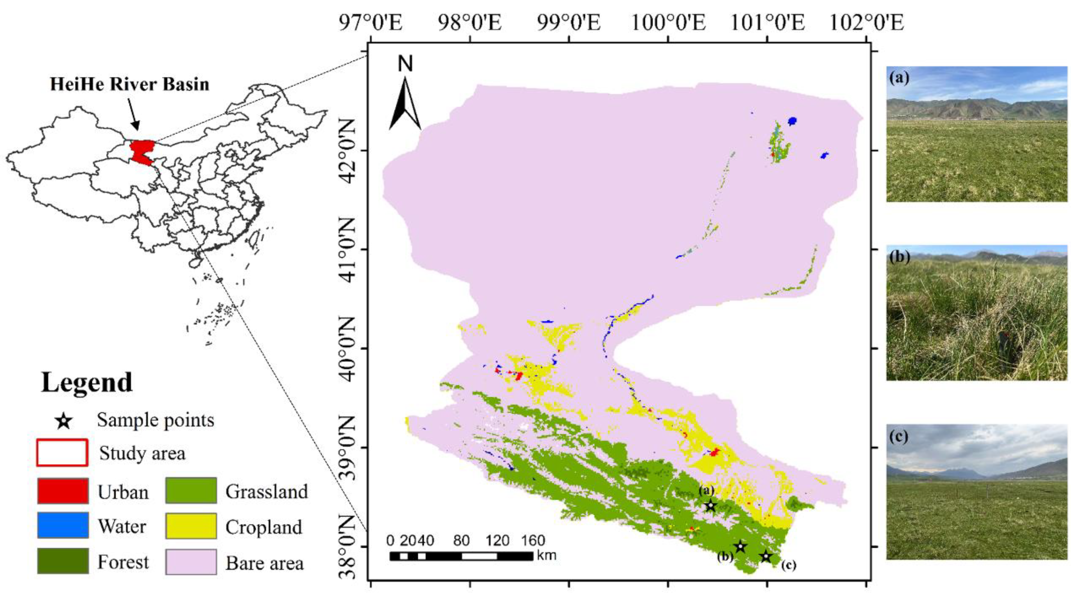
2.1. Study Area

The Heihe River Basin (HRB, 37.7°–42.7°N and 97.1–102.0°E) is the second largest inland river basin in northwestern China, covering 12.8 × 10⁴ km², and belongs to an arid–semiarid climate zone (Figure 1). The elevation ranges from 716 to 5583 m asl [27], and the mean annual precipitation is 200–500 mm [28]. High-resolution VOD products would be of great value for the ecological and environmental management in HRB. The land cover in the study area is highly heterogeneous from high to low altitudes, where major vegetation types are grasslands [29] followed by croplands and forests [30].

This study focused on the VOD retrievals over grasslands of the HRB (Figure 1), and the growing season of grassland was from May to October. Thus, the study period was from May to October, 2018–2020.

2.2. Sentinel-1 A Data

The S1 SAR satellite belongs to Europe’s Copernicus program and currently consists of two satellites in orbit, Sentinel-1A and Sentinel-1B, launched in April 2014 and 2016, respectively [31]. New generation S1 satellites provide wide-swath TOPSAR images at the C-band (5.045 GHz) in VH and VV polarizations [32], with a total swath width of 250 km and 12 days repeat for a single track. S1 data can be downloaded from the Sentinel-1 Data Hub website (https://scihub.copernicus.eu/, accessed on 1 May 2021). Only Sentinel-1A data are available over the study area. The VOD retrieved from VV polarization has a better performance based on the previous studies that retrieved VOD from C-band radar data [8,20]. Thus, the descending backscatter data product of Sentinel-1A at VV-polarization was used here. Three years (2018–2020) of 10 m Level-1 Ground-Range Detected at High resolution (GRDH) products (in Interferometric Wide Swath acquisition mode) were used in the present study.

The ESA Sentinels Application Platform (SNAP) software package was used to pre-process the backscatter data into the normalized backscatter [33]. The procedure to process SAR data using Sentinel Toolbox is given as follows: (1) apply orbit data; (2) thermal noise; (3) calibrate SAR data to obtain beta-naught (${\beta }^0$); (4) speckle; (5) local incidence angle correction to obtain gamma-naught (${\gamma }^0$) using SRTM-1 DEM (radiometric terrain flattening); (6) foreshortening correction using SRTM-1 DEM (range-doppler terrain correction). Accounting for the noise of S1 sensors and the limitation of spatial resolution of auxiliary datasets used in our proposed algorithm, the backscatter dataset was resampled to 1 km using the linear average method.

Note that the normalized backscatter ${\gamma }^0$ was used in this study instead of sigma-naught (${\sigma }^0$) and beta-naught (${\beta }^0$). The ${\gamma }^0$ uses the area projected along the line of site and is suitable for looking at volume scattering [34], i.e.,

$${\gamma }^0=\frac{{\sigma }^0}{cos \theta }$$

(1)

where θ is the local incidence angle.

In addition, the effects of topography on ${\gamma }^0$ were removed. The prevalence of steep slopes in the study area may introduce the artifacts of the DEM product, potentially resulting in uncertainties in the terrain normalization during the SNAP process [35]. To reduce the influence of steep slopes, slope data and the standard deviation (std) of DEM (DEM_std) were used to filter outlier pixels with slopes > 8° and DEM_std > 100 m.

2.3. Soil Moisture Data

The ERA5 SM data are from the fifth generation Climate Change Service (C3S) [36]. The hourly ERA5 soil column is discretized into four soil layers (0–7, 7–28, 28–100, 100–289 cm) with a spatial resolution of 0.25°. Considering that S1 (descending) observations are obtained at 11:00 AM local solar time (LST), only the topsoil layer (0–7 cm) outputs at 11:00 LST were used between 2018 and 2020.

To study the sensitivity of S1 VOD retrievals to the source of SM data, we also explored SM from the GLDAS-Noah (version 2.1) [37], with a spatial resolution from 0.25° × 0.25° and a temporal resolution of 3-hourly. The top 0–10 cm GLDAS SM data in the present study were from 6:00 AM LST.

To obtain the same spatial resolution as the S1 data (1 km), all SM data were considered as spatially homogeneous within with each pixel and resampled to a spatial resolution of 1 km using the nearest neighbor interpolation method.

2.4. MODIS Vegetation Indices

Various vegetation indices (VIs), including NDVI, EVI, and LAI, were utilized to assess the performance of VOD products. In addition, NDVI was used to calibrate the soil and vegetation model parameters.

The 1 km MODIS NDVI and EVI data were extracted from the 8 day MODIS product (MOD13A2 [38] and MYD13A2 [39]), and the 500 m MODIS LAI data were obtained from the 4-day MCD15A3H [40]. For retaining high-quality VIs observations, we masked out poor-quality pixels using the respective flags provided by the MODIS products (pixel reliability = 0). The Sentinel-2 (S2) VIs were calculated in the Google Earth Engine (GEE) platform by using images (cloud-free) from Sentinel-2 data. These VIs data were then aggregated to 1 km by using the linear averaging method to match the S1 grid.

Due to the inconsistent overpass time of MODIS and Sentinel-1, VIs data were temporally matched to the closest S1 observation. The time of each VI products and S1 data were matched within a maximum time interval of 4 days. In line with previous studies, the vegetation dynamics represented by VIs were assumed to be stable during the four days, and similar assumptions were used in [20].

2.5. Land Cover Data

The 300 m land cover data, provided by ESA Climate Change Initiative Land Cover (CCI-LC) maps in 2015 [30] (https://www.esa-landcover-cci.org/, accessed on 1 September 2021), were used to assist in the calibration of soil model parameters [8] and to select the VOD data of grassland. To match the S1 data, the CCI-LC map was aggregated at 1 km by selecting the maximum cover fraction from their original resolution.

2.6. Land Surface Parameters

Several land surface variables and parameters (Table S1) were used to train the soil model parameters, including soil properties, terrain parameters, and dynamic soil temperature (ST). These data have an important impact on the SM and the signal acquired from the microwave observations [41,42]. We divided these data into two categories to observe the importance of two categories of variables for the soil model parameters, respectively. The soil properties were retrieved from the SoilGrids250m dataset with a spatial resolution of 250 m, which is an automated system for global digital soil mapping that uses machine learning methods to map the spatial distribution of soil properties [43]. The average value of the 0–5 cm depths of twelve soil property data was used here.

The terrain parameters (e.g., elevation, slope, curvature, roughness, etc.) (Table S1) were calculated using the Digital Elevation Model (DEM) provided by the Global Multi-resolution Terrain Elevation Data 2010 (GMTED2010) for 15-arc-second spatial resolutions [44]. These parameters were finally aggregated to 1 km using a simple averaging method to match the spatial resolution of S1.

The 0.25° daily ST data were obtained from ERA5 [45]. The topsoil layer (0–7 cm) and 11:00 UTC data were selected to match the S1 overpass.

3. Methodology

3.1. Water Cloud Model

To simplify the scattering mechanism for low vegetation cover such as grassland, the WCM assumes: (1) the “clouds” representing vegetation are uniformly distributed throughout space [45,46], and (2) only a single scattering needs to be considered [47]. Therefore, the total backscatter in the linear scale (${\gamma }_{obs}^o$) can be defined as two components, namely, the vegetation volume backscattering (${\gamma }_{vege}^o$), and the soil backscattering (${\gamma }_{soil}^o$), expressed in Equation (2). The soil component of the backscatter ${\gamma }_{soil}^o$ is attenuated by the vegetation transmissivity (${\beta }^2$). ${\beta }^2$ is closely related to VOD and can be expressed in Equation (3) [48].

$${\gamma }_{obs}^o={\gamma }_{vege}^o+{\beta }^2{\gamma }_{soil}^o$$

(2)

$${\beta }^2=exp\left[-2 VOD/cos \theta \right]$$

(3)

where $\theta$ is the incidence angle, which was normalized to 0°.

The backscatter from vegetation (${\gamma }_{vege}^0$) can be calculated as:

$${\gamma }_{vege}^0=A{V}_{1}cos \theta \left(1-{\beta }^2\right)$$

(4)

$A$ is the vegetation parameter, representing the vegetation canopy backscatter under dense vegetation coverage. The $V_1$ is usually equal to one [25]. In very dense vegetation regions (VDV), where the soil effects could be neglected, it can be assumed that the vegetation transmissivity approaches zero (${\beta }^2=0$) [8], and Equation (2) can be simplified as follows:

$${\gamma }_{obs}^o={\gamma }_{vege}^o=Acos \theta$$

(5)

where the $A$ value in VDV (described as $A_0$) can be expressed using the following function:

$$A_0={\gamma }_{obs}^o/cos \theta$$

(6)

$A\left(i,j,t\right)$ was set spatially homogenously equal to $A_0^{95\%}\left(t\right)$, which is the 95th percentile of $A_0\left(i,j\right)$ over all VDV pixels $\left(i,j\right)$ at day t (assuming all pixels have the same $A_0\left(t\right)$ value at time t) [8]:

$$A\left(i,j,t\right)=A_0^{95\%}\left(t\right)$$

(7)

Studies have found that better performances in retrievals were obtained with the WCM model when different $A$ values were set for different types of land cover [26]. Therefore, we computed the $A_0\left(t\right)$ value only using the $A_0\left(i,j\right)$ over VDV in grassland.

Note that VDV pixels, which were used for the calculation of $A_0\left(i,j\right)$, were defined as the pixels where the NDVI values were larger than the 75th percentile of the NDVI time series (Equation (8)).

$$NDV{I}_{VDV}>NDV{I}^{75\%}\left(t\right)$$

(8)

In times without VDV, the soil has an important influence, and ${\gamma }_{soil}^o$ (in dB) was in this study expressed using the Ulaby model [49] as follows:

$${\gamma }_{soil\left(dB\right)}^0=D\ast SM+C$$

(9)

where $C$ and $D$ are the soil parameters, $C$ is the backscattering coefficient under very dry situations, and $D$ parameterizes the sensitivity of the backscatter data to SM. The calibration of parameters $C$ and $D$ are described in Section 3.2.

Combined with the Equations (2)–(4) and (9), VOD can be expressed as

$$VOD=-1/2cos \theta ln\left(\frac{{\gamma }_{obs}^o-Acos \theta }{{10}^{0.1\left(C+D\ast SM\right)}-Acos \theta }\right)$$

(10)

using a spatially constant $A$ parameter and spatially variant $C$ and $D$ parameters, as shown in the flowchart of Figure 2, and further described below.

3.2. Calibration of the Soil Model

The key to construct a soil model is to calibrate $C$ and $D$ (Equation (9)). We calibrated $C$ and $D$ for each year individually in order to avoid the effects of temporal and spatial variations in SM and backscatters [50]. The annual bare soil regions were selected to train the calibration model of $C$ and $D$, and the calibrated model was subsequently used to estimate $C$ and $D$ over all of the regions (e.g., bare soil and vegetation-covering regions) using a random forest (RF) regression algorithm. The details of the calibration procedure are described below and illustrated in Figure 2:

(1) The selection of bare soil pixels.

We assumed that vegetation effects could be neglected in bare soil time steps, which were defined as either: "bare soil" based on the CCI-LC type, or within the vegetation sparse period with NDVI lower than 0.1.

(2) The calibration of soil parameters over the bare soil pixels.

Given the significant relationship between ${\gamma }_{soil}^o$ and SM, there are two conditions to compute the annual soil parameters $C$ and $D$:

Category 1: for pixels where ${\gamma }_{soil}^o$ is sensitive to SM, a linear relationship could be computed between ${\gamma }_{soil\left(dB\right)}^o$ and SM (Equation (9)). The pixels were defined as a subset of those identified in (1), i.e., they refer to the bare soil time steps being greater than 30% of the entire number of observations, and the standard deviation of the time series of ${\gamma }_{soil}^o$ and SM should be greater than 1.63 dB and 0.015 ${\mathrm{m}}^3/{\mathrm{m}}^3$ in 2018, 1.62 dB and 0.014 ${\mathrm{m}}^3/{\mathrm{m}}^3$ in 2019, and 1.64 dB and 0.015 ${\mathrm{m}}^3/{\mathrm{m}}^3$ in 2020, respectively. To ensure a robust and physically-based linearity, the annual values of $C$ and $D$ were only retained over the regions having a significantly positive relationship (expressed by Equation (9)) between ${\gamma }_{obs\left(dB\right)}^0$ and SM.

Category 2: for a subset of pixels identified in (1), where SM is consistently under very dry conditions, and the ${\gamma }_{obs\left(dB\right)}^0$ is assumed to be almost constant, the annual $C$ parameter was calculated as the mean value of the ${\gamma }_{soil}^o$ (Equation (11)). The standard deviation of the time series of ${\gamma }_{soil}^o$ and SM should be greater than 1.62 dB and 0.014 ${\mathrm{m}}^3/{\mathrm{m}}^3$, respectively, and the number of SM data below 0.1 ${\mathrm{m}}^3/{\mathrm{m}}^3$ should be greater than 80% of the entire number of observations:

$$C=average \left({\gamma }_{soil}^0\right)$$

(11)

(3) The calibration of the soil parameters ($C$ and $D$) over all of the regions.

Based on the results above (for category 1 and category 2), we used the land surface parameters (Table S1) as predictors to train two random forest (RF) regression models for the annual spatial pattern of $C$ and $D$ over the study area separately. RF regression is a machine learning method that has the advantage of being a nonlinear and nonparametric method, and the contribution of each predictor to the target that is computed by the RF model is very useful for tuning the model. There are 27 predictors for each soil model parameter, and collinearity exists among them. In order to achieve the best prediction of annual $C$ and $D$, the training procedure was repeated iteratively by removing the least essential predictors in each step to find the optimum combination of predictors for the $C$ and $D$ parameters separately (the amount of trees was set to 80). After this training step, the two trained RF models were used to calibrate the annual $C$ and $D$ parameters over the whole study area.

4. Results

4.1. Calibration of Soil Parameters

4.1.1. The Calibration Results of the $C$ over the Whole Region

Taking 2018 as an example, 10,469 pixels (Equation (9)) and 28,808 (Equation (11)) bare soil pixels were used to train the $C$ parameter, which were mainly located in the northern part of the study area (Figure 3a), and $C$ values having a mean value of −15.75 ± 4.40 dB in a range from −40 to 0 dB (Figure 3c). Based on the training data above, a random forest model was developed to estimate $C$ values over the whole study area. In total, 15 variables were chosen to train the RF model of $C$, including 10 soil properties and 5 terrain data (Figure 4). Cation exchange capacity (Cation), Soil organic carbon stock (C stock), and mean value of elevation (DEM mean) were the three most important variables. Those three variables can explain around 30% of the target. The $C$ value corresponds to the radar backscatter in very dry conditions, and the pixels used to calibrate the $C$ value were located in the topographically flat areas; therefore, the soil properties data had a greater impact in the $C$ model.

The scatterplot between the calibrated and RF predicted values for the $C$ showed the model for the $C$ estimates performed quite well, indicated by R = 0.95, and RMSE = 1.40 dB (Figure 3d). The predicted $C$ values ranged from −40 to 0 dB and were generally higher in the north than in the south, showing a spatial pattern of a declining trend from the northern to the central and to the southern parts of the region (Figure 3b). Similar results for the calibrated $C$ were also observed in 2019 and 2020 (Figures S1 and S2).

4.1.2. The Retrieval of the $D$ over all of the Regions

In total, 10,469 pixels in 2018 were selected to train the $D$ parameter based on Equation (9) to train the calibration model of $D$, which were mainly distributed in the north of the study area (Figure 5a), with $D$ values having a mean value of 37.25 ± 19.63 $\mathrm{dB}/{\mathrm{m}}^3{\ast \mathrm{m}}^{-3}$ in a range from 10 to 90 $\mathrm{dB}/{\mathrm{m}}^3{\ast \mathrm{m}}^{-3}$ (Figure 5c). Based on the training data above, 15 variables were selected to train the RF model of $D$, including 10 soil properties and 5 terrain data (Figure 6). DEM mean, sand total (Sand), and terrain surface texture (TST) were found to be the most important variables. Those three variables could explain around 29.6% of the target. The $D$ value represented the sensitivity of the radar data to soil moisture, and the pixels used to calibrate the $D$ value were located in mountainous areas and were greatly influenced by the topography. Therefore, the contribution of the terrain data (related to topography) in the $D$ value model was, as expected, larger than that in the $C$ value model.

The RF model could predict the $D$ values effectively (R = 0.92, RMSE = 8.23 $\mathrm{dB}/{\mathrm{m}}^3{\ast \mathrm{m}}^{-3}$), with predicted $D$ in a range from 10 to 90 $\mathrm{dB}/{\mathrm{m}}^3{\ast \mathrm{m}}^{-3}$ (Figure 5d). The predicted $D$ values in the southern area were generally higher than those in the northern areas, showing a spatial pattern of an ascending trend from the northern to the central and to the southern parts of the region (Figure 5b). Similar results of the calibrated $D$ were also observed in 2019 and 2020 (Figures S3 and S4).

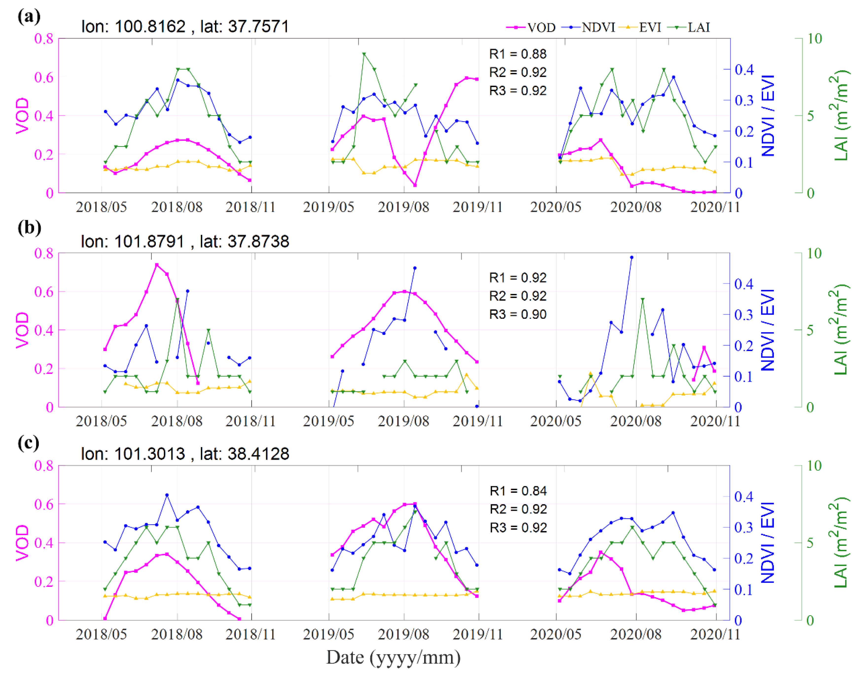
4.2. Evaluation of VOD against MODIS VIs

Figure 7a–c show that the retrievals of VOD in the three years (2018–2020) had similar spatial patterns: the highest values were distributed in the central and eastern parts of the study area, with VOD values between 0.2 and 0.3, and the southern region presented low to medium VOD values, between 0 and 0.1. Figure 7d–f show the histograms of VOD in 2018, 2019, and 2020 with mean VODs of 0.18 ± 0.16, 0.20 ± 0.28, 0.25 ± 0.23, respectively. Figure 8 shows that the VOD estimates had a well-marked seasonal variability, with vegetation growth and biomass increases; VOD gradually increased in spring and reached a peak in summer and then decreased during fall with the senescence of the vegetation.

To assess the intra-annual performance of the VOD estimates in the monitoring of the vegetation dynamics, the temporal correlation (R) between VOD and VIs for the years 2018, 2019, and 2020 are shown in Figure 9. For the comparisons between VOD and NDVI, the mean R values were 0.70, 0.74, and 0.82 in 2018, 2019, and 2020, respectively. Similar good performances were also observed from the comparisons of VOD with EVI (having mean R values of 0.69, 0.70, and 0.81 in the three years) and with LAI (having mean R values of 0.69, 0.74, and 0.80 for each of the three years). The overall R values over 2018–2020 were 0.76, 0.75, and 0.75 for NDVI, LAI, and EVI, respectively. These results suggest that the VOD estimates have good performance in monitoring vegetation dynamics over the study area, and that the intra-annual variability (within a year) is typically captured rather than the interannual variability between years.

The spatial patterns of the temporal R values between VOD and VIs are shown in Figure 10. The R values between VOD and VIs were high in the middle of the study area (Figure 10a–l), albeit with different R values over the parts of the region. VOD retrievals were better correlated with NDVI/EVI than LAI over most of study area (Figure 11). The percentage of pixels with the highest correlation for each VIs data point is given in Figure 11b. VOD had the highest correlation with NDVI at over 49.53%, followed by LAI (17.45%) and EVI (33.01%).

In addition, we also evaluated the VOD estimates against S2 VIs. The R between VOD and VIs for the year 2018 is shown in Figure 12. The highest spatial correlation values were obtained with EVI (R = 0.74), followed by NDVI (R = 0.72) and LAI (R = 0.72). Results showed that the spatial relationship between VOD and S2 VIs was higher than the relationship between VOD and MODIS VIs, likely because the S2 VIs data were more temporally matched to the S1 observation than MODIS VIs.

To better understand the performance of VOD, we further looked into three well-performing sites to show the changes in VOD and VIs, as seen in Figure 8. First, it is important to highlight that VOD retrievals were available every 12 days, whereas the optical VIs were often missing due to cloud contamination. For all sites, the time series of VOD estimates showed the obvious seasonal variability of VOD estimates: VOD increased gradually and reached a peak in summer with vegetation growth and biomass increase, followed by the decreased VOD during fall as vegetation began to senesce. In general, VOD had good sensitivity to VIs (e.g., R value between VOD and NDVI (EVI, LAI) was 0.89 (0.90, 0.90) at the first site (Figure 8a). VOD and VIs values generally peaked synchronously, suggesting that the VWC was the maximum with the highest LAI and NDVI values.

5. Discussion

Our results showed that the proposed approach can accurately retrieve VOD at high resolution over grassland using S1 images. Yet, the proposed VOD retrieval algorithm has some uncertainties caused by the accuracy of SM used as input, the thresholds of R value between SM and ${\gamma }_{soil}^0$ in the soil model, and other factors (topographic features, the uncertainties in optical VIs), which will be discussed in the following sub-sections.

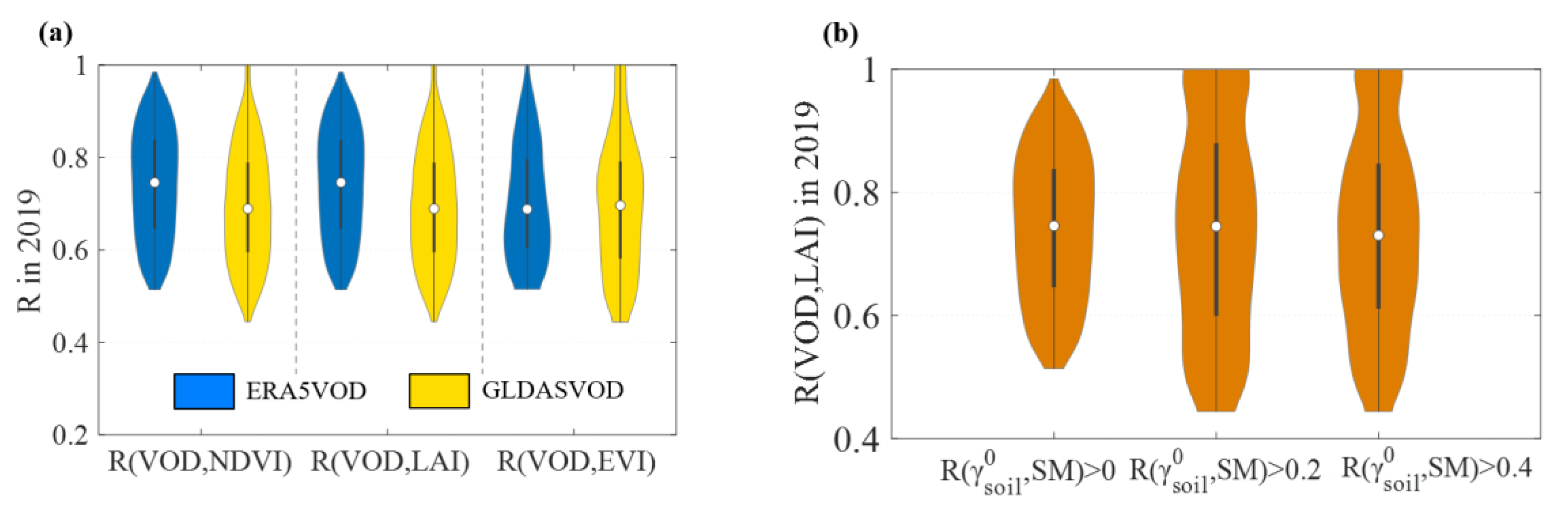
5.1. Impact of Soil Moisture on the VOD Retrieval

An accurate SM value is the key to VOD retrievals, because the accuracy of ${\gamma }_{soil}^0$ values in the soil model (see Equation (9)) highly depends on the SM. For example, a sensitivity analysis by El Hajj et al. (2019) showed that a 5 vol.% underestimation in SM could lead to an underestimation of the VOD value by 0.02 [20]. Liu et al. (2021) also discovered that an underestimation (overestimation) in SM of 0.05 ${\mathrm{m}}^3/{\mathrm{m}}^3$ would result in an underestimation (overestimation) of 0.02 in VOD over grassland [8]. In our study, the long-term value of SM and its consequence in terms of VOD magnitude is not a primary cause of uncertainty, because the $C$ and $D$ parameters might compensate for the long-term SM values. However, the temporal variability in SM will affect the short-term or intra-annual variability of the VOD retrievals. Although many SM products are available, validation results have indicated that most SM products have significant uncertainties [51,52,53], which will increase the uncertainties of VOD retrievals.

Thus, four SM products (e.g., SMAP-L3 [54], SMOS-IC [55], GLDAS, ERA5 SM) as inputs in the soil model (Equation (9)) were tested in our proposed algorithm to better understand the impact of SM accuracy on the VOD retrievals, but the results are only shown for GLDAS and ERA5 SM, because SMOS and SMAP retrievals are hampered by complex topography in this region (as brightness temperatures measured by radiometers are flagged/discarded in the presence of topography due to the strong influence of this parameter on microwave radiation). Figure 12a displays the correlation between VIs (NDVI, LAI, EVI) and VOD retrievals using two SM products (from GLDAS and ERA5) for the year 2019, respectively. VOD retrieved by ERA5 (ERA5VOD) shows the best performance (mean R = 0.74, 0.74, 0.70 for NDVI, LAI, EVI, respectively), followed by VOD retrieved by GLDAS (GLDASVOD) (mean R = 0.69, 0.69, 0.70 for NDVI, LAI, EVI, respectively), confirming that SM is important for retrieving VOD in our algorithm.

Furthermore, the proposed algorithm assumed that the SM within the 25 km × 25 km area is equal in each 1 km pixel due to the limitation of the coarse resolution of SM products. Note that the assumption has high uncertainties over large regions because the SM is known to present large heterogeneities caused by changes in meteorological conditions and soil properties at a small scale [56]. However, high-resolution (e.g., 1 km) SM is not operationally available in the study area. Future downscaling of existing products could be developed to increase the spatial resolution of SM products [57,58,59,60], which will improve the accuracy of the current VOD retrievals.

5.2. Impact of the Soil Parameters $C$ and $D$ on VOD Retrievals

The soil parameters ($C$ and $D$) used in the soil model (Equation (9)) are keys to the simulation of ${\gamma }_{soil}^0$. The soil parameters were determined by a threshold of R values greater than 0 between SM and ${\gamma }_{obs}^0$. Indeed, the determination of the threshold could strongly influence the performance of VOD retrievals, thus different thresholds of the R values between SM and ${\gamma }_{obs}^0$ were tested in the soil model to understand the impact of soil parameters on VOD retrievals.

Here, three R values between ${\gamma }_{soil}^0$ and SM, including R > 0, R > 0.2, and R > 0.4, were used to determine the soil parameters (Equation (9)). Results showed that VOD had the highest correlations (mean R = 0.74 with LAI in 2019) when the threshold of the R value was zero (Figure 13b). It should be noted that the higher R values used to determine soil parameters did not improve the VOD retrievals, as indicated by the low R values between VOD and VIs. This may be because a higher R value threshold will lead to fewer pixels to train the RF model, potentially resulting in uncertainty in model performance [61].

5.3. Impact of Other Factors on VOD Retrievals

Note that over some of the study area, low correlation values between VOD and VIs were observed spatially, which can be attributed to two factors:

(1) Topographic complexity. Although the topographic effect was corrected using topographic normalization during our pre-processing to correct the location of each pixel [33], slope steepness and slope direction had a complex effect on radar backscattering [62]. Topographic normalization in pre-processes cannot completely remove the impact of terrain in complex terrains, because the DEM products (e.g., SRTM or TanDEM-X DEM) used in topographic normalization may not be able to normalize SAR backscatter radiometrically under complex topographic conditions [62,63].

(2) Limits of evaluation methods. A direct validation of the VODs is not possible because of the lack of consensus on reference values from in situ measurements or models [64]. Most evaluations of VOD datasets are based on a side-by-side comparison with proxies of the vegetation greenness based on optical vegetation indices (e.g., [8,9,14,65,66,67,68]), including NDVI, EVI, and LAI. These previous comparisons revealed that VOD can generally capture vegetation seasonal cycles and interannual variations in a similar fashion as vegetation indices. Therefore, we used three optical vegetation-related parameters (e.g., NDVI, LAI and EVI) to evaluate the accuracy of VOD retrievals from a spatial perspective, as was done in [64]. Nevertheless, the difference in variation between VOD and VIs can also be interpreted as VOD, representing the VWC, which contains different information than VIs (NDVI is more sensitive to chlorophyll in leaves, LAI represents the vegetation density, and EVI responds more strongly to the canopy type and structure). This could lead to time lags and variations in dynamics between their time series [65,69]. Noting these limits, we think the chosen evaluation metrics are effective for the assessment of VOD retrievals in this study, as several studies have shown that VOD has high spatial-temporal coherence with optical VIs, especially in short vegetation areas [8,65], while our study area is mainly covered by grasslands (Figure 1). Uncertainties in the optical VIs could partly explain their low correlation with VOD retrievals over parts of the study area. For example, cloud cover and aerosols [70] may cause poor data quality and significant missing daily values, resulting in VIs that may not always represent vegetation change. In addition, the unmatched footprints between MODIS VIs and S1 could be another reason for the low agreement between VOD and VIs. Therefore, in situ-measured VWC and higher temporal resolution VIs (such as using Sentinel-2 for calculation VIs) can be used for further validation of the VOD in future studies.

6. Conclusions

We proposed an approach to estimate high-resolution VOD over grassland in a region in the Heihe River basin using an analytic solution of a simplified WCM. Specifically, the algorithm is constrained by the given SM estimates, and the vegetation backscatter at full vegetation cover ($A$ parameter) is assumed to be homogenous, which limits the algorithm to uniform land cover regions with limited climate differences. The relationship between backscatter and SM ($C$, $D$ parameters) is calibrated at bare pixels and extrapolated to the entire grassland region via RF and using soil, temperature, and terrain properties as predictors.

The temporal dynamics of the retrieved VOD agree well with optical VIs (the mean R across the three years 2018–2020 is 0.76, 0.75, 0.75 for NDVI, LAI, and EVI, respectively). However, some uncertainties, such as the accuracy of SM and topography could all affect the accuracy of VOD estimates. The next step will concentrate on enhancing the algorithm developed in this study and applying it to other land cover types in other areas to improve the accuracy of VOD. In addition, comparisons could be made with in situ-measured VWC to provide a more robust evaluation of VOD estimates.

References

- Frappart, F.; Wigneron, J.-P.; Li, X.; Liu, X.; Al-Yaari, A.; Fan, L.; Wang, M.; Moisy, C.; Le Masson, E.; Lafkih, Z.A.; et al. Global Monitoring of the Vegetation Dynamics from the Vegetation Optical Depth (VOD): A Review. Remote Sens. 2020, 12, 2915. [Google Scholar] [CrossRef]
- Jackson, T.; Schmugge, T. Vegetation effects on the microwave emission of soils. Remote Sens. Environ. 1991, 36, 203–212. [Google Scholar] [CrossRef]
- Wigneron, J.-P.; Parde, M.; Waldteufel, P.; Chanzy, A.; Kerr, Y.; Schmidl, S.; Skou, N. Characterizing the Dependence of Vegetation Model Parameters on Crop Structure, Incidence Angle, and Polarization at L-Band. IEEE Trans. Geosci. Remote Sens. 2004, 42, 416–425. [Google Scholar] [CrossRef]
- Vittucci, C.; Vaglio Laurin, G.; Tramontana, G.; Ferrazzoli, P.; Guerriero, L.; Papale, D. Vegetation optical depth at L-band and above ground biomass in the tropical range: Evaluating their relationships at continental and regional scales. Int. J. Appl. Earth Obs. Geoinf. 2019, 77, 151–161. [Google Scholar] [CrossRef]
- Ulaby, F.T.; Long, D.G.; Blackwell, W.J.; Elachi, C.; Fung, A.K.; Ruf, C.; Sarabandi, K.; Zebker, H.A.; Van Zyl, J. Micro-Wave Radar and Radiometric Remote Sensing; University of Michigan Press: Ann Arbor, MI, USA, 2014; Volume 4. [Google Scholar]
- Momen, M.; Wood, J.D.; Novick, K.A.; Pangle, R.; Pockman, W.T.; McDowell, N.G.; Konings, A.G. Interacting Effects of Leaf Water Potential and Biomass on Vegetation Optical Depth. J. Geophys. Res. Biogeosci. 2017, 122, 3031–3046. [Google Scholar] [CrossRef]
- Vreugdenhil, M.; Dorigo, W.A.; Wagner, W.; de Jeu, R.A.M.; Hahn, S.; van Marle, M.J.E. Analyzing the Vegetation Pa-rameterization in the TU-Wien ASCAT Soil Moisture Retrieval. IEEE Trans. Geosci. Remote Sens. 2016, 54, 3513–3531. [Google Scholar] [CrossRef]
- Liu, X.; Wigneron, J.-P.; Fan, L.; Frappart, F.; Ciais, P.; Baghdadi, N.; Zribi, M.; Jagdhuber, T.; Li, X.; Wang, M.; et al. ASCAT IB: A radar-based vegetation optical depth retrieved from the ASCAT scatterometer satellite. Remote Sens. Environ. 2021, 264, 112587. [Google Scholar] [CrossRef]
- Karthikeyan, L.; Pan, M.; Konings, A.G.; Piles, M.; Fernandez-Moran, R.; Kumar, D.N.; Wood, E.F. Simultaneous retrieval of global scale Vegetation Optical Depth, surface roughness, and soil moisture using X-band AMSR-E observations. Remote Sens. Environ. 2019, 234, 111473. [Google Scholar] [CrossRef]
- Wang, M.; Fan, L.; Frappart, F.; Ciais, P.; Sun, R.; Liu, Y.; Li, X.; Liu, X.; Moisy, C.; Wigneron, J.-P. An alternative AMSR2 vegetation optical depth for monitoring vegetation at large scales. Remote Sens. Environ. 2021, 263, 112556. [Google Scholar] [CrossRef]
- Fernandez-Moran, R.; Al-Yaari, A.; Mialon, A.; Mahmoodi, A.; Al Bitar, A.; De Lannoy, G.; Rodriguez-Fernandez, N.; Lopez-Baeza, E.; Kerr, Y.; Wigneron, J.-P. SMOS-IC: An Alternative SMOS Soil Moisture and Vegetation Optical Depth Product. Remote Sens. 2017, 9, 457. [Google Scholar] [CrossRef]
- Li, X.; Wigneron, J.-P.; Fan, L.; Frappart, F.; Yueh, S.H.; Colliander, A.; Ebtehaj, A.; Gao, L.; Fernandez-Moran, R.; Liu, X.; et al. A new SMAP soil moisture and vegetation optical depth product (SMAP-IB): Algorithm, assessment and inter-comparison. Remote Sens. Environ. 2022, 271, 112921. [Google Scholar] [CrossRef]
- Qin, Y.; Xiao, X.; Wigneron, J.-P.; Ciais, P.; Brandt, M.; Fan, L.; Li, X.; Crowell, S.; Wu, X.; Doughty, R.; et al. Carbon loss from forest degradation exceeds that from deforestation in the Brazilian Amazon. Nat. Clim. Chang. 2021, 11, 442–448. [Google Scholar] [CrossRef]
- Jones, M.O.; Jones, L.A.; Kimball, J.S.; McDonald, K.C. Satellite passive microwave remote sensing for monitoring global land surface phenology. Remote Sens. Environ. 2011, 115, 1102–1114. [Google Scholar] [CrossRef]
- Liu, H.; Zhan, Q.; Yang, C.; Wang, J. Characterizing the Spatio-Temporal Pattern of Land Surface Temperature through Time Series Clustering: Based on the Latent Pattern and Morphology. Remote Sens. 2018, 10, 654. [Google Scholar] [CrossRef]
- Fan, L.; Wigneron, J.-P.; Xiao, Q.; Al-Yaari, A.; Wen, J.; Martin-StPaul, N.; Dupuy, J.-L.; Pimont, F.; Al Bitar, A.; Fernandez-Moran, R.; et al. Evaluation of microwave remote sensing for monitoring live fuel moisture content in the Mediterranean region. Remote Sens. Environ. 2018, 205, 210–223. [Google Scholar] [CrossRef]
- Vreugdenhil, M.; Navacchi, C.; Bauer-Marschallinger, B.; Hahn, S.; Steele-Dunne, S.; Pfeil, I.; Dorigo, W.; Wagner, W. Sentinel-1 Cross Ratio and Vegetation Optical Depth: A Comparison over Europe. Remote Sens. 2020, 12, 3404. [Google Scholar] [CrossRef]
- Piles, M.; Entekhabi, D.; Camps, A. A Change Detection Algorithm for Retrieving High-Resolution Soil Moisture From SMAP Radar and Radiometer Observations. IEEE Trans. Geosci. Remote Sens. 2009, 47, 4125–4131. [Google Scholar] [CrossRef]
- Owe, M.; de Jeu, R.; Walker, J. A methodology for surface soil moisture and vegetation optical depth retrieval using the microwave polarization difference index. IEEE Trans. Geosci. Remote Sens. 2001, 39, 1643–1654. [Google Scholar] [CrossRef]
- El Hajj, M.; Baghdadi, N.; Wigneron, J.-P.; Zribi, M.; Albergel, C.; Calvet, J.-C.; Fayad, I. First Vegetation Optical Depth Mapping from Sentinel-1 C-band SAR Data over Crop Fields. Remote Sens. 2019, 11, 2769. [Google Scholar] [CrossRef]
- Veloso, A.; Mermoz, S.; Bouvet, A.; Le Toan, T.; Planells, M.; Dejoux, J.-F.; Ceschia, E. Understanding the temporal behavior of crops using Sentinel-1 and Sentinel-2-like data for agricultural applications. Remote Sens. Environ. 2017, 199, 415–426. [Google Scholar] [CrossRef]
- Vreugdenhil, M.; Wagner, W.; Bauer-Marschallinger, B.; Pfeil, I.; Teubner, I.; Rüdiger, C.; Strauss, P. Sensitivity of Senti-nel-1 Backscatter to Vegetation Dynamics: An Austrian Case Study. Remote Sens. 2018, 10, 1396. [Google Scholar] [CrossRef]
- Lievens, H.; Martens, B.; Verhoest, N.; Hahn, S.; Reichle, R.; Miralles, D. Assimilation of global radar backscatter and radiometer brightness temperature observations to improve soil moisture and land evaporation estimates. Remote Sens. Environ. 2017, 189, 194–210. [Google Scholar] [CrossRef]
- Shamambo, D.C.; Bonan, B.; Calvet, J.-C.; Albergel, C.; Hahn, S. Interpretation of ASCAT Radar Scatterometer Observations Over Land: A Case Study Over Southwestern France. Remote Sens. 2019, 11, 2842. [Google Scholar] [CrossRef]
- Attema, E.P.W.; Ulaby, F.T. Vegetation modeled as a water cloud. Radio Sci. 1978, 13, 357–364. [Google Scholar] [CrossRef]
- Bindlish, R.; Barros, A.P. Parameterization of vegetation backscatter in radar-based, soil moisture estimation. Remote Sens. Environ. 2001, 76, 130–137. [Google Scholar] [CrossRef]
- Cheng, G.; Li, X.; Liu, S.; Xiao, Q.; Ma, M.; Jin, R.; Che, T.; Liu, Q.; Wang, W.; Qi, Y.; et al. Heihe Watershed Allied Telemetry Experimental Research (HiWATER): Scientific Objectives and Experimental Design. Bull. Am. Meteorol. Soc. 2013, 94, 1145–1160. [Google Scholar]
- Wang, G.; Cheng, G. Land desertification status and developing trend in the Heihe river basin. J. Desert Res. 1999, 19, 368–374. [Google Scholar]
- Che, T.; Li, X.; Liu, S.; Li, H.; Xu, Z.; Tan, J.; Zhang, Y.; Ren, Z.; Xiao, L.; Deng, J.; et al. Integrated hydrometeorological, snow and frozen-ground observations in the alpine region of the Heihe River Basin, China. Earth Syst. Sci. Data 2019, 11, 1483–1499. [Google Scholar] [CrossRef]
- ESA. Land Cover CCI Product User Guide Version 2; Technical Report; ESA: Paris, France, 2017. [Google Scholar]
- Torres, R.; Snoeij, P.; Geudtner, D.; Bibby, D.; Davidson, M.; Attema, E.; Potin, P.; Rommen, B.; Floury, N.; Brown, M.; et al. GMES Sentinel-1 mission. Remote Sens. Environ. 2012, 120, 9–24. [Google Scholar] [CrossRef]
- Xu, B.; Li, Z.-W.; Zhu, Y.; Shi, J.; Feng, G. Kinematic Coregistration of Sentinel-1 TOPSAR Images Based on Sequential Least Squares Adjustment. IEEE J. Sel. Top. Appl. Earth Obs. Remote Sens. 2020, 13, 3083–3093. [Google Scholar] [CrossRef]
- Filipponi, F. Sentinel-1 GRD Preprocessing Workflow. Multidiscip. Digit. Publ. Inst. Proc. 2019, 18, 11. [Google Scholar]
- Woodhouse, I.H. Introduction to Microwave Remote Sensing; TayloCRC & Fprancies Group: Boca Raton, FL, USA, 2006. [Google Scholar]
- Purinton, B.; Bookhagen, B. Validation of digital elevation models (DEMs) and comparison of geomorphic metrics on the southern Central Andean Plateau. Earth Surf. Dyn. 2017, 5, 211–237. [Google Scholar] [CrossRef]
- Hersbach, H.; Dee, D. ERA5 Reanalysis is in Production. ECMWF Newsletter. 2016, Volume 147, p. 7. Available online: https://www.ecmwf.int/en/newsletter/147/news/era5-reanalysis-production (accessed on 3 October 2020).
- Rodell, M.; Houser, P.; Jambor, U.; Gottschalck, J.; Mitchell, K.; Meng, C.-J.; Arsenault, K.; Cosgrove, B.; Radakovich, J.; Bosilovich, M. The global land data assimilation system. Bull. Am. Meteorol. Soc. 2004, 85, 381–394. [Google Scholar] [CrossRef]
- Didan, K. MOD13A2 MODIS/Terra Vegetation Indices 16-Day L3 Global 1 km SIN Grid V006. 2015. distributed by NASA EOSDIS Land Processes DAAC. Available online: https://lpdaac.usgs.gov/products/mod13a2v006/ (accessed on 28 June 2021).
- Didan, K. MYD13A2 MODIS/Aqua Vegetation Indices 16-Day L3 Global 1 km SIN Grid V006. 2015. distributed by NASA EOSDIS Land Processes DAAC. Available online: https://lpdaac.usgs.gov/products/myd13a2v006/ (accessed on 28 June 2021).
- Myneni, R.; Knyazikhin, Y.; Park, T. MCD15A3H MODIS/Terra+Aqua Leaf Area Index/FPAR 4-day L4 Global 500 m SIN Grid V006. 2015. distributed by NASA EOSDIS Land Processes DAAC. Available online: https://lpdaac.usgs.gov/products/mcd15a3hv006/ (accessed on 28 June 2021).
- Blanco, C.M.G.; Gomez, V.M.B.; Crespo, P.; Ließ, M. Spatial prediction of soil water retention in a Páramo landscape: Methodological insight into machine learning using random forest. Geoderma 2018, 316, 100–114. [Google Scholar] [CrossRef]
- Chunfeng, M.; Xin, L.; Shuguo, W. A Global Sensitivity Analysis of Soil Parameters Associated With Backscattering Using the Advanced Integral Equation Model. IEEE Trans. Geosci. Remote Sens. 2015, 53, 5613–5623. [Google Scholar] [CrossRef]
- Hengl, T.; De Jesus, J.M.; Heuvelink, G.B.M.; Gonzalez, M.R.; Kilibarda, M.; Blagotić, A.; Shangguan, W.; Wright, M.N.; Geng, X.; Bauer-Marschallinger, B.; et al. SoilGrids250m: Global gridded soil information based on machine learning. PLoS ONE 2017, 12, e0169748. [Google Scholar] [CrossRef]
- Danielson, J.J.; Gesch, D.B. Global Multi-Resolution Terrain Elevation Data 2010 (GMTED2010); US Department of the Interior, US Geological Survey: Washington, DC, USA, 2011. [Google Scholar]
- Hersbach, H.; Bell, B.; Berrisford, P.; Hirahara, S.; Horányi, A.; Muñoz-Sabater, J.; Simmons, A. The ERA5 global reanalysis. Q. J. R. Meteorol. Soc. 2020, 146, 1999–2049. [Google Scholar] [CrossRef]
- Park, S.E.; Jung, Y.T.; Cho, J.H.; Moon, H.; Han, S.H. Theoretical Evaluation of Water Cloud Model Vegetation Parameters. Remote Sens. 2019, 11, 894. [Google Scholar] [CrossRef]
- Chauhan, S.; Srivastava, H.S.; Patel, P. Improved Parameterization of Water Cloud Model for Hybrid-Polarized Backscatter Sim-ulation Using Interaction Factor. Int. Arch. Photogramm. Remote Sens. Spat. Inf. Sci. 2017, 42, 61–66. [Google Scholar] [CrossRef]
- Baghdadi, N.; El Hajj, M.; Zribi, M.; Bousbih, S. Calibration of the Water Cloud Model at C-Band for Winter Crop Fields and Grasslands. Remote Sens. 2017, 9, 969. [Google Scholar] [CrossRef]
- Ulaby, F.T.; Batlivala, P.P.; Dobson, M.C. Microwave Backscatter Dependence on Surface Roughness, Soil Moisture, and Soil Texture: Part I-Bare Soil. IEEE Trans. Geosci. Electron. 1978, 16, 286–295. [Google Scholar] [CrossRef]
- El Hajj, M.; Baghdadi, N.; Zribi, M.; Angelliaume, S. Analysis of Sentinel-1 Radiometric Stability and Quality for Land Surface Applications. Remote Sens. 2016, 8, 406. [Google Scholar] [CrossRef]
- Ma, C.; Li, X.; Wei, L.; Wang, W. Multi-Scale Validation of SMAP Soil Moisture Products over Cold and Arid Regions in Northwestern China Using Distributed Ground Observation Data. Remote Sens. 2017, 9, 327. [Google Scholar] [CrossRef]
- Yao, Y.; Zhang, Y.; Liu, Q.; Liu, S.; Jia, K.; Zhang, X.; Xu, Z.; Xu, T.; Chen, J.; Fisher, J.B. Evaluation of a satellite-derived model parameterized by three soil moisture constraints to estimate terrestrial latent heat flux in the Heihe River basin of Northwest China. Sci. Total Environ. 2019, 695, 133787. [Google Scholar] [CrossRef] [PubMed]
- Lu, Z.; Chai, L.; Zhang, T.; Cui, H.; Wang, J.; Li, W. Validation of SMOS soil moisture production in the Heihe River Basin of China. In Proceedings of the IEEE International Geoscience & Remote Sensing Symposium, Beijing, China, 10–15 July 2016. [Google Scholar] [CrossRef]
- Chan, S.K.; Bindlish, R.; O’Neill, P.E.; Njoku, E.; Jackson, T.; Colliander, A.; Chen, F.; Burgin, M.; Dunbar, S.; Piepmeier, J.; et al. Assessment of the SMAP Passive Soil Moisture Product. IEEE Trans. Geosci. Remote Sens. 2016, 54, 4994–5007. [Google Scholar] [CrossRef]
- Wigneron, J.-P.; Li, X.; Frappart, F.; Fan, L.; Al-Yaari, A.; De Lannoy, G.; Liu, X.; Wang, M.; Le Masson, E.; Moisy, C. SMOS-IC data record of soil moisture and L-VOD: Historical development, applications and perspectives. Remote Sens. Environ. 2020, 254, 112238. [Google Scholar] [CrossRef]
- Crow, W.T.; Berg, A.A.; Cosh, M.H.; Loew, A.; Mohanty, B.P.; Panciera, R.; de Rosnay, P.; Ryu, D.; Walker, J.P. Upscaling sparse ground-based soil moisture observations for the validation of coarse-resolution satellite soil moisture products. Rev. Geophys. 2012, 50, 1. [Google Scholar] [CrossRef]
- Song, P.; Huang, J.; Mansaray, L.R. An improved surface soil moisture downscaling approach over cloudy areas based on geo-graphically weighted regression. Agric. For. Meteorol. 2019, 275, 146–158. [Google Scholar] [CrossRef]
- Long, D.; Bai, L.; Yan, L.; Zhang, C.; Yang, W.; Lei, H.; Quan, J.; Meng, X.; Shi, C. Generation of spatially complete and daily continuous surface soil moisture of high spatial resolution. Remote Sens. Environ. 2019, 233. [Google Scholar] [CrossRef]
- Zhao, W.; Wen, F.; Wang, Q.; Sanchez, N.; Piles, M. Seamless downscaling of the ESA CCI soil moisture data at the daily scale with MODIS land products. J. Hydrol. 2021, 603, 126930. [Google Scholar] [CrossRef]
- Peng, J.; Albergel, C.; Balenzano, A.; Brocca, L.; Cartus, O.; Cosh, M.H.; Crow, W.T.; Dabrowska-Zielinska, K.; Dadson, S.; Davidson, M.W.; et al. A roadmap for high-resolution satellite soil moisture applications – confronting product characteristics with user requirements. Remote Sens. Environ. 2020, 252, 112162. [Google Scholar] [CrossRef]
- Breiman, L. Random forests. Mach. Learn. 2001, 45, 5–32. [Google Scholar] [CrossRef]
- Hoekman, D.H.; Reiche, J. Multi-model radiometric slope correction of SAR images of complex terrain using a two-stage semi-empirical approach. Remote Sens. Environ. 2015, 156, 1–10. [Google Scholar] [CrossRef]
- Borlaf-Mena, I.; Santoro, M.; Villard, L.; Badea, O.; Tanase, M.A. Investigating the Impact of Digital Elevation Models on Sentinel-1 Backscatter and Coherence Observations. Remote Sens. 2020, 12, 3016. [Google Scholar] [CrossRef]
- Li, X.; Al-Yaari, A.; Schwank, M.; Fan, L.; Frappart, F.; Swenson, J.; Wigneron, J.-P. Compared performances of SMOS-IC soil moisture and vegetation optical depth retrievals based on Tau-Omega and Two-Stream microwave emission models. Remote Sens. Environ. 2019, 236, 111502. [Google Scholar] [CrossRef]
- Du, J.; Kimball, J.S.; Jones, L.A.; Kim, Y.; Glassy, J.; Watts, J.D. A global satellite environmental data record derived from AMSR-E and AMSR2 microwave Earth observations. Earth Syst. Sci. Data 2017, 9, 791–808. [Google Scholar] [CrossRef]
- Grant, J.; Wigneron, J.-P.; De Jeu, R.; Lawrence, H.; Mialon, A.; Richaume, P.; Al Bitar, A.; Drusch, M.; Van Marle, M.; Kerr, Y. Comparison of SMOS and AMSR-E vegetation optical depth to four MODIS-based vegetation indices. Remote Sens. Environ. 2016, 172, 87–100. [Google Scholar] [CrossRef]
- Lawrence, H.; Wigneron, J.-P.; Richaume, P.; Novello, N.; Grant, J.; Mialon, A.; Al Bitar, A.; Merlin, O.; Guyon, D.; Leroux, D.; et al. Comparison between SMOS Vegetation Optical Depth products and MODIS vegetation indices over crop zones of the USA. Remote Sens. Environ. 2014, 140, 396–406. [Google Scholar] [CrossRef]
- Liu, Y.Y.; de Jeu, R.A.M.; McCabe, M.F.; Evans, J.P.; van Dijk, A.I.J.M. Global long-term passive microwave satellite-based retrievals of vegetation optical depth. Geophys. Res. Lett. 2011, 38, 1. [Google Scholar] [CrossRef]
- Pfeil, I.; Vreugdenhil, M.; Hahn, S.; Wagner, W.; Strauss, P.; Blöschl, G. Improving the Seasonal Representation of ASCAT Soil Moisture and Vegetation Dynamics in a Temperate Climate. Remote Sens. 2018, 10, 1788. [Google Scholar] [CrossRef]
- Forkel, M.; Carvalhais, N.; Verbesselt, J.; Mahecha, M.D.; Neigh, C.S.R.; Reichstein, M. Trend Change Detection in NDVI Time Series: Effects of Inter-Annual Variability and Methodology. Remote Sens. 2013, 5, 2113–2144. [Google Scholar] [CrossRef]
Publisher’s Note: MDPI stays neutral with regard to jurisdictional claims in published maps and institutional affiliations. |
© 2022 by the authors. Licensee MDPI, Basel, Switzerland. This article is an open access article distributed under the terms and conditions of the Creative Commons Attribution (CC BY) license (https://creativecommons.org/licenses/by/4.0/).
Share and Cite
Zhou, Z.; Fan, L.; De Lannoy, G.; Liu, X.; Peng, J.; Bai, X.; Frappart, F.; Baghdadi, N.; Xing, Z.; Li, X.; et al. Retrieval of High-Resolution Vegetation Optical Depth from Sentinel-1 Data over a Grassland Region in the Heihe River Basin. Remote Sens. 2022, 14, 5468. https://doi.org/10.3390/rs14215468
Zhou Z, Fan L, De Lannoy G, Liu X, Peng J, Bai X, Frappart F, Baghdadi N, Xing Z, Li X, et al. Retrieval of High-Resolution Vegetation Optical Depth from Sentinel-1 Data over a Grassland Region in the Heihe River Basin. Remote Sensing. 2022; 14(21):5468. https://doi.org/10.3390/rs14215468
Chicago/Turabian StyleZhou, Zhilan, Lei Fan, Gabrielle De Lannoy, Xiangzhuo Liu, Jian Peng, Xiaojing Bai, Frédéric Frappart, Nicolas Baghdadi, Zanpin Xing, Xiaojun Li, and et al. 2022. "Retrieval of High-Resolution Vegetation Optical Depth from Sentinel-1 Data over a Grassland Region in the Heihe River Basin" Remote Sensing 14, no. 21: 5468. https://doi.org/10.3390/rs14215468
APA StyleZhou, Z., Fan, L., De Lannoy, G., Liu, X., Peng, J., Bai, X., Frappart, F., Baghdadi, N., Xing, Z., Li, X., Ma, M., Li, X., Che, T., Geng, L., & Wigneron, J.-P. (2022). Retrieval of High-Resolution Vegetation Optical Depth from Sentinel-1 Data over a Grassland Region in the Heihe River Basin. Remote Sensing, 14(21), 5468. https://doi.org/10.3390/rs14215468