Article

An Adaptive Joint Bilateral Interpolation-Based Color Blending Method for Stitched UAV Images

Department of Computer Science and Information Engineering, National Taiwan University of Science and Technology, Taipei 10672, Taiwan
*
Author to whom correspondence should be addressed.
Remote Sens. 2022, 14(21), 5440; https://doi.org/10.3390/rs14215440
Submission received: 26 August 2022 / Revised: 25 October 2022 / Accepted: 26 October 2022 / Published: 29 October 2022
(This article belongs to the Special Issue Computer Vision and Image Processing)

Abstract

:
Given a source UAV (unmanned aerial vehicle) image I s and a target UAV image I t , it is a challenging problem to correct the color of all target pixels so that the subjective and objective quality effects between I s and I t can be as consistent as possible. Recently, by referring to all stitching color difference values on the stitching line, a global bilateral joint interpolation-based (GBJI-based) color correction method was proposed. However, because all stitching color difference values may contain aligned and misaligned stitching pixels, the GBJI-based method suffers from a perceptual artifact near the misaligned stitching pixels. To remedy this perceptual artifact, in this paper, we propose an adaptive joint bilateral interpolation-based (AJBI-based) color blending method such that each target pixel only adaptively refers to an adequate interval of stitching color difference values locally. Based on several testing stitched UAV images under different brightness and misalignment situations, comprehensive experimental results demonstrate that in terms of PSNR (peak signal-to-noise ratio), SSIM (structural similarity index), and FSIM (feature similarity index), our method achieves higher objective quality effects and also achieves better perceptual effects, particularly near the misaligned stitching pixels, when compared with the GBJI-based method and the other state-of-the-art methods.

Graphical Abstract

1. Introduction

Due to the advance of unmanned aerial vehicle (UAV) technologies, the images captured by UAV are cost- and time-effective. In addition, they can provide high quality geographic data and information from a low flight altitude. These advantages make UAV images an increasingly popular medium for many applications [1,2,3,4,5,6], such as disaster assessment, construction site monitoring, building change detection, military applications, and heating requirement determination for frost management. However, the area that one UAV image can cover is limited by the flight altitude. Therefore, to extend the area that UAV images can cover, the method of stitching UAV images has received extensive attention.
To construct a stitched image, several seam cutting-based methods [7,8,9,10,11,12] have been developed. They often include the image registration step, the seam searching step, and the color blending step. In the image registration step, the feature points [13] are first extracted from the source image I s and the target image I t to establish the correspondence [14,15,16,17] between I s and I t , and then according to the established correspondence, a proper perspective transform is performed on the target image I t such that the source image I s and the transformed target image can be aligned as well as possible. After that, the overlapping area of I s and I t can be determined. The seam searching step is used to determine the best stitching line to separate the overlapping area of I s and I t into two disjoint parts.
Let Ω s and Ω t denote the pixel sets on the side of the stitching line in I s and I t , respectively, where Ω s Ω t = . Usually, the color inconsistency problem is caused by different exposure times, atmosphere illuminations, and different capturing times between I s and I t , and it makes the stitched image visually unpleasant. In this study, we focus on addressing the color consistency correction problem for the target pixels in Ω t to make the stitched image have good subjective and objective quality performance. Note that each stitching target pixel on the stitching line is only updated by simply adding the corresponding stitching color difference to the color of that stitching target pixel. In the next subsection, the classical representative works in the color consistency correction area, as well as their advantages and shortcomings, are introduced.

1.1. Related Works

Brown and Lowe [18] proposed a multi-band blending (MBB) method to correct color in low frequency over a large spatial range, and to correct color in high frequency over a short spatial range. Their method could produce a smooth color transition across the warped overlapping area of I s and I t , denoted by O s , t w , but it cannot effectively solve the color inconsistency problem in the area I t - O s , t w , where the operator “-” denotes a set difference operator. Fecker et al. [19] proposed a histogram matching-based (HM-based) method to correct color between I s and I t . They first built up the cumulative histograms of I s and I t , respectively, and then a mapping function was delivered to correct the color of each target pixel in I t . Although the HM-based method is very fast, it lacks the pixel position consideration in the cumulative histograms used, limiting the color correction effect.
Xiong and Pulli [20] proposed a two-step approach to correct color. First they applied a gamma function to modify the luminance component for the target pixels, and then applied a linear correction function to modify the chrominance components. Based on a parameterized spline curve approach for each image, Xia et al. [21] proposed a new gradient preservation-based (GP-based) color correction method. Using the convex quadratic programming technique, a closed form was derived to model the color correction problem by considering the visual quality of I s and I t as well as the global color consistency. To enhance the accuracy of the extracted color correspondence, the gradient and color features in the possible alteration objects in O s , t were utilized. However, the single-channel optimization strategy used in the GP-based method was unable to solve the white balance problem. Later, based on a spline curve remapping function and the structure from motion technique, Yang et al. [22] proposed a global color correction method for large-scale image sets in three-dimensional reconstruction applications.
Fang et al. [23] found that in the stitched image, the stitching pixel set information on the stitching line is useful for color blending, but this information is ignored in the above-mentioned related color blending methods. Utilizing all color difference values on the stitching line globally for each target pixel, Fang et al. proposed a global joint bilateral interpolation-based (GJBI-based) color blending method. Based on several testing stitched images, each one with well aligned stitching pixels, their experimental results demonstrated the visual quality superiority of their method over the MBB method, the HM-based method, Xiong and Pulli’s method, and the GP-based method.
Parallel to the above introduction on color correction for stitched images, for multiple images, some color correction methods have been developed and they include the joint global and local color consistency approach [24], the combined model color correction approach [25], and the contrast-aware color consistency approach [26].

1.2. Motivation

The GJBI-based method [23] achieved good visual quality performance for well stitched images, in which one stitched image almost contains aligned stitching pixels without parallax distortion. In practical situations, one stitched image often has not only aligned stitching pixels but also has misaligned stitching pixels. From the experimental data, we found that the GJBI-based method tends to suffer from a perceptual artifact near the misaligned stitching pixel set, in which each stitching color difference between the source pixel and the target pixel becomes conspicuous due to parallax distortion.
The above perceptual artifact occurring in the GJBI-based method motivated us to propose a new adaptive joint bilateral interpolation-based (AJBI-based) color blending method, such that instead of referring to all stitching color difference values on the stitching line globally, each target pixel only adaptively refers to an adequate interval of stitching color difference values locally, achieving a better subjective quality effect near the misaligned stitching pixels and a higher objective quality benefit.

1.3. Contributions

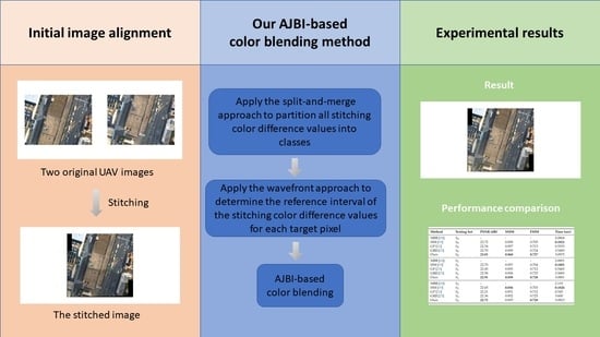
In this paper, we propose an AJBI-based color blending method to correct the color for the stitched UAV images. The contributions of the proposed method are clarified below.
  • We first propose a split-and-merge approach to classify all stitching color difference values into one aligned class or two classes, namely the aligned class C a corresponding to aligned stitching pixels and the misaligned class C m corresponding to misaligned stitching pixels. Next, we propose a wavefront approach to determine the adequate reference interval of the stitching color difference values, which will be used for correcting the color of each target pixel in Ω t ;
  • To remedy the perceptual artifact near the misaligned stitching pixels, instead of using all stitching color difference values globally, we propose an AJBI-based method to correct color for each target pixel in Ω t by using the determined reference stitching color difference values locally. It is notable that in the Gaussian function used in our method for correcting color for each target pixel, the color variance parameter setting (see Equation (6)) is adaptively dependent on the ratio of the number of all reference misaligned stitching color differences over the number of all reference stitching color difference values;
  • Based on several tests of UAV stitched images under different misalignment and brightness situations, the comprehensive experimental results justify that in terms of the three objective quality metrics, namely PSNR (peak signal-to-noise ratio), SSIM (structural similarity index) [27], and FSIM (feature similarity index) [28], the proposed AJBI-based color blending method achieves higher objective quality effects when compared with the state-of-the-art methods [18,19,21,23]. In addition, relative to these comparative methods, the proposed color blending method also achieves better perceptual effects, particularly near the misaligned stitching pixels.
The rest of this paper is organized as follows. In Section 2, the proposed split-and-merge approach to classify all stitching color difference values into one aligned class or two different classes is presented. In Section 3, the proposed AJBI-based color blending method is presented. In Section 4, thorough experiments are carried out to justify the better color consistency correction merit of the proposed method. In Section 5, the conclusions and future work are addressed.

2. The Classification of Stitching Color Difference Values

In this section, we first take one real stitched image example to define the stitching color difference values on the stitching line, and then the proposed split-and-merge approach is presented to partition all stitching color difference values into one aligned class or two classes, namely the aligned class and the misaligned class. Based on the same stitched image example, the partition result using the proposed split-and-merge approach is also provided. To help clarify the visual understanding of the proposed approach, a flowchart is also provided.
Given I s and I t in Figure 1a, after performing Yuan et al.’s superpixel- and graph cut-based method [10] on Figure 1a, Figure 1b shows the resultant stitched image, where the stitching line is marked in red and the overlapping area between I s and I t is shown by an area surrounded by a green quadrilateral. On the stitching line with n pixel-pairs, namely ( p s ( i ) , p t ( i ) ) for 1 <= i <= n, p s ( i ) and p t ( i ) denote the ith stitching source pixel and target pixel, respectively. The stitching color difference value between p s ( i ) and p t ( i ) is defined by
D ( p s > t ( i ) ) = C ( p s ( i ) ) C ( p t ( i ) )
where C ( p s ( i ) ) and C ( p t ( i ) ) denote the color values of p s ( i ) and p t ( i ) , respectively.
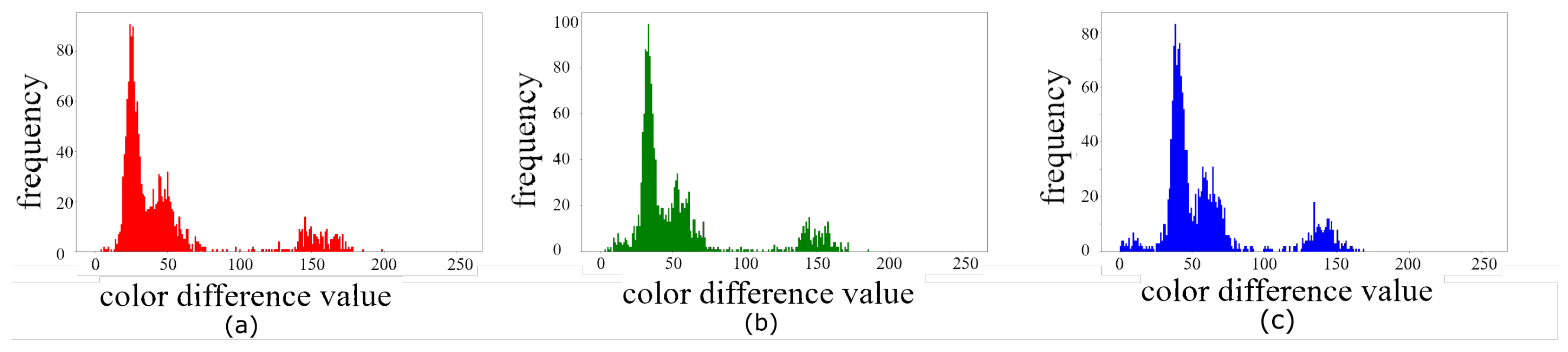
On the stitching line, let D a , c ( p s > t ( i ) ) denote the absolute stitching c-color difference value between p s ( i ) and p t ( i ) ; it is defined by
D a , c ( p s > t ( i ) ) = | C c ( p s ( i ) ) C c ( p t ( i ) ) |
where C c ( p s ( i ) ) and C c ( p t ( i ) ) denote the c-color, c ∈ {R, G, B}, values of p s ( i ) and p t ( i ) , respectively. For the stitching line in Figure 1b, the three distributions of D R ( p s > t ) , D G ( p s > t ) , and D B ( p s > t ) are shown in Figure 2a, Figure 2b, and Figure 2c, respectively. From Figure 2a–c, we can observe that the three distributions of all absolute stitching c-color difference values tend to be two classes, namely the aligned class and the misaligned class.
We propose a split-and-merge approach to partition all stitching c-color, c ∈ {R, G, B}, difference values into two classes, C a and C m , or one aligned class. In most cases, all stitching color difference values on the stitching line tend to be partitioned into two classes, namely C a and C m . However, for the rare example, the distribution of all absolute stitching c-color difference values tends to be one aligned class. As depicted in Figure 3, a flowchart is provided to help clarify the visual understanding of the proposed split-and merge approach.
When setting K = 2, we first adopt Lloyd’s K-means clustering process [29] to split all absolute stitching color difference values, which constitute the feature space used in the clustering process, into two tentative classes, C a and C m . Initially, two randomly selected absolute stitching color difference values form the centers of the two tentative classes. Next, based on the minimal 2-norm distance criterion, every absolute color difference value is assigned to one class center. Then, the center of each class is updated by the mean value of all absolute color difference values in the same class. The above procedure is repeated until two stable classes are found. Then, we propose a merging cost-based process to examine whether the two tentative classes can be merged into one aligned class C a or not. If the two tentative classes cannot be merged into one class, we report the two tentative classes as the partition result; otherwise, we report the aligned class C a as the partition result. It can be said that our split-and-merge approach consists of one two-means splitting process and one merging process.
Let the variances of C a , C m , and C a be denoted by σ C a 2 , σ C m 2 , and σ C a 2 , respectively; let n be the number of all stitching color difference values, and let μ C a and μ C m be the mean values of the absolute color difference values in C a and C m , respectively. The three variances, σ C a 2 , σ C m 2 , and σ C a 2 , have the relation in Theorem 1, and the merging cost term “ | C a | | C m | n 2 ( μ C a μ C m ) 2 ” in Theorem 1 is used to determine whether the two different classes, C a and C m , can be merged into one aligned class C a or not.
Theorem 1.
σ C a 2 = w a σ C a 2 + w m σ C m 2 + | C a | | C m | n 2 ( μ C a μ C m ) 2 where w a = C a n , w m = C m n , and 1 = w a + w m .
The above theorem is proved in the Appendix A.
In Theorem 1, if the merging cost term “ | C a | | C m | n 2 ( μ C a μ C m ) 2 ” is larger than or equal to the specified threshold T c o s t , it indicates that the split two classes, C a and C m , cannot be merged into one aligned class C a ; otherwise, the class C a and the class C m should be merged into one class C a . In our experience, after trying the interval [100, 1000], the best choice of T c o s t is recommended to be set to 500.
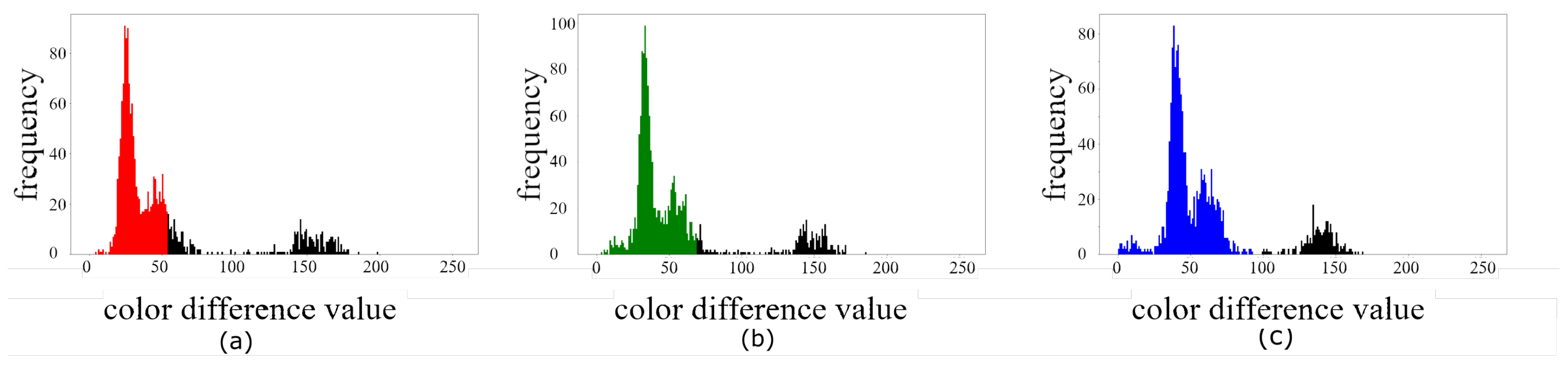
After performing our split-and-merge approach on the three distributions in Figure 2a–c, Figure 4a–c illustrate the corresponding classification results, where the aligned absolute c-color difference class C a , c ∈{R, G, B}, is depicted in c-color, and the misaligned absolute c-color difference class C m is depicted in black. 
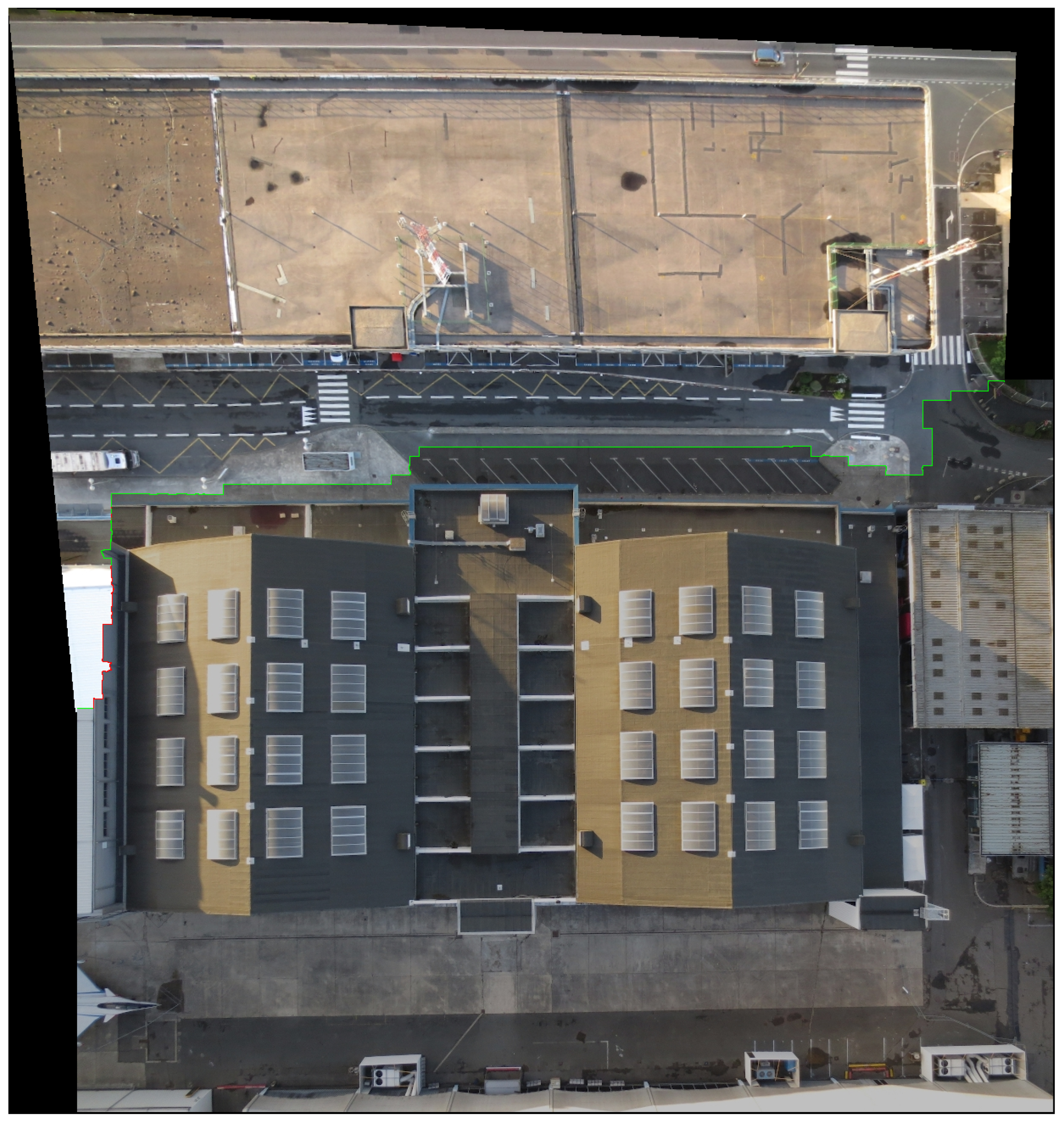
Figure 5 depicts the partition result of Figure 1b, where on the stitching line, the aligned color difference pixels are marked in green color and the misaligned color difference pixels are marked in red color.

3. The Proposed Adaptive Color Blending Method

Based on the two partitioned classes of the stitching color difference values using the proposed split-and-merge approach, we first propose a wavefront approach to determine the adequate reference interval of stitching c-color difference values, and then we propose an adaptive joint bilateral interpolation-based (AJBI-based) color blending method to improve the color correction effect, particularly achieving a better perceptual color consistency effect near the misaligned stitching pixels.

3.1. The Proposed Wavefront Approach

For easy exposition, we take an example to explain the proposed wavefront approach. As depicted in Figure 6, the stitching target pixels on the stitching line are labeled as brown, and they constitute the initial wavefront W ( 0 ) .
Next, the target pixels ( Ω t ) neighboring W ( 0 ) constitute the first wavefront W ( 1 ) , and these target pixels in W ( 1 ) are labeled as red. We continue the wavefront marching-based labelling operations until all wavefronts are constructed. As depicted in Figure 6, there are 12 constructed wavefronts for the target pixels in Ω t . It can be easily verified that the proposed wavefront approach takes O ( | Ω t | ) time, where the big-O notation denotes an upper bound complexity [30], to construct all wavefronts for all target pixels in Ω t . Let the resultant wavefronts be denoted by W ( 0 ) , W ( 1 ) , …, and W ( m ) with | Ω t | = i = 1 m | W ( i ) | , where the wavefront number m depends on the stitching line configuration and | Ω t | .
Let the jth target pixel in the kth wavefront W ( k ) be denoted by p t ( j ) , 1 <= j <= | W ( k ) | and 1 <= k. For the target pixel p t ( j ) in W ( k ) , let N ( p t ( j ) ) denote the neighboring target pixel set in the wavefront W ( k 1 ) , where the cardinality of N ( p t ( j ) ) may be 1, 2, 3, 4, or 5. For example, in Figure 6, for the three target pixels, namely B, C, and E, in W ( 1 ) , the cardinalities of their neighboring target pixel sets in W ( 0 ) are 2, 3, and 4, respectively. For the target pixel A in W ( 3 ) , the cardinality of its neighboring target pixel set in W ( 2 ) is 1. For the target pixel D in W ( 10 ) , the cardinality of its neighboring target pixel set in W ( 9 ) is 4.
For each stitching target pixel p t ( i ) in the initial wavefront W ( 0 ) , 1 <= i <= | W ( 0 ) | , p t ( i ) only refers to its own stitching color difference value at the same position to correct the color. For each target pixel p t ( j ) in W ( 1 ) , p t ( j ) mainly refers to the stitching color difference values in N ( p t ( j ) ) in W ( 0 ) , and it also can refer to some extra left q stitching color difference values of N l e f t ( p t ( j ) ) and the extra right q stitching color difference values of N r i g h t ( p t ( j ) ) , where N l e f t ( p t ( j ) ) and N r i g h t ( p t ( j ) ) denote the leftmost and rightmost target pixels in N ( p t ( j ) ) , respectively. Empirically, the specified value q could be selected from the interval [2, 20]. Generally, for each target pixel p t ( j ) in W ( k ) , 1 <= k <= m, its reference interval of the stitching color difference values in W ( 0 ) , denoted by R ( p t ( j ) ) , can be determined iteratively.

3.2. The Proposed AJBI-Based Color Blending Method

By utilizing the reference stitching color difference values of each target pixel in Ω t , we propose an AJBI-based color blending method. Initially, for each stitching target pixel p t ( i ) , 1 <= i <= | W ( 0 ) | , we correct its color by summing up its own color value C ( p t ( i ) ) and the stitching color difference value D ( p s > t ( i ) ) (see Equation (1)) by
C ( p t ( i ) ) : = C ( p t ( i ) ) + D ( p s > t ( i ) )
After correcting the color for all stitching target pixels in W ( 0 ) by Equation (3), for each target pixel p t in Ω t , based on the reference stitching color difference values of p t , namely R ( p t ) , and the original color of p t , we correct the color of p t by using the following joint bilateral interpolation:
C ( p t ) : = C ( p t ) + p R ( p t ) ω p [ D ( p ) ]
with
ω p = exp ( | | C ( p t ) C ( p ) | | 2 σ c o l o r 2 ) * exp ( | | P ( p t ) P ( p ) | | 2 σ d i s t a n c e 2 ) p ^ R ( p t ) exp ( | | C ( p t ) C ( p ^ ) | | 2 σ c o l o r 2 ) * exp ( | | P ( p t ) P ( p ^ ) | | 2 σ d i s t a n c e 2 )
where P ( p t ) , P ( p ) , and P ( p ^ ) denote the x-y coordinates of the target pixel p t , the stitching target pixel p , and the stitching target pixel p ^ , respectively. The deviation σ c o l o r in Equation (5) is defined as follows:
σ c o l o r = m a x ( c * | R ( p t ) m i s a l i g n e d | | R ( p t ) | , c m i n )
where R ( p t ) m i s a l i g n e d denotes the misaligned stitching target pixel set corresponding to the reference stitching color difference values in R ( p t ) . c and c m i n are user defined parameters, and they are set to c = 3 and c m i n = 0.1 in our experiment. In Equation (6), the higher the value of | R ( p t ) m i s a l i g n e d | | R ( p t ) | , the higher the value setting for σ c o l o r .
Since every target pixel in Ω t performing color correction only refers to its own reference interval of the stitching color difference values in W ( 0 ) , by Equation (4), the color correction of each target pixel can be done in parallel to accelerate the color correction process.

4. Experimental Results

Based on the eight original testing UAV image-pairs, which are selected from the website: https://www.sensefly.com/education/datasets (accessed on 2 September 2018) provided by the company “senseFly”, the corresponding eight stitched images are produced by using Yuan et al.’s graph cut-based method [10]. The eight testing stitched images can be accessed from the website in Supplementary Material. For convenience, let the resultant eight stitched images under different misalignment situations be denoted by the set symbol S 0 with | S 0 | = 8. For each stitched image in S 0 , the misalignment ratio of the stitching color difference values is within the interval [0%, 15%].
Based on the testing set S 0 under different misalignment situations, to produce more stitched images under different brightness situations, for each testing stitched image in S 0 , the brightness of every pixel in the target image is updated by four different brightness percentages, namely −15%, 15%, −25%, and 25%, of its own brightness. Here, if the updated brightness of one target pixel is over the range [0, 255], it is forced to be 0 or 255. Figure 7a illustrates one stitched image taken from S 0 , where the stitching line is depicted by a green line. Figure 7b illustrates the updated stitched image of Figure 7a, where the brightness of the target image in Figure 7b is obtained by increasing the 15% brightness percentage of that in Figure 7a. In Figure 7b, we can observe that the target image, which is below the stitching line, is brighter than the corresponding target image in Figure 7a. Therefore, for each original testing stitched image, four updated stitched images are produced. Overall, 32 (4 × 8) newly generated stitched images are produced. Among the 32 generated stitched images that can be accessed from the website in Supplementary Material, the 16 newly generated stitched images under ± 15 % brightness update are denoted by the set symbol S 1 with | S 1 | = 16, and the 16 newly generated stitched images under ± 25 % brightness update are denoted by the set symbol S 2 with | S 2 | = 16. Here, for each stitched image in S 1 , the misalignment ratio of the stitching color difference values is within the interval [0%, 37%]; for each stitched image in S 2 , the misalignment ratio of the stitching color difference values is within the interval [0%, 32%].
Next, the proposed split-and-merge approach is applied to partition the color difference values of the stitching line of each testing stitched image in S 0 , S 1 , and S 2 , into two classes. After performing the proposed split-and-merge approach on the stitching color difference values of Figure 7b, the misaligned part of the stitching line in Figure 7c is marked in red color and the aligned part is marked in green color. Based on the 40 testing stitched images in S 0 , S 1 , and S 2 , comprehensive experimental results demonstrate the objective and subjective quality merits of the proposed AJBI-based color correction method relative to the 4 comparative methods, namely the MBB method [18], the HM-based method [19], the GP-based method [21], and the GBJI-based method [23]. Here, the three objective quality metrics, namely PSNR, SSIM, and FSIM, are used to justify the objective quality merit of the proposed color blending method. In addition, the visual demonstration is provided to justify the subjective quality merit of the proposed method. The execution time comparison is also reported.
Among the four comparative methods, the execution code of the MBB method [18] can be accessed from the website: http://matthewalunbrown.com/autostitch/autostitch.html (accessed on 23 October 2021). The C++ source code of the GP-based method [21] can be accessed from the website: https://github.com/MenghanXia/ColorConsistency (accessed on 29 August 2021). We have tried our best to implement the HM-based method [19] and the GJBI-based method [23] in C++ language. The blending parameters of the GJBI-based method are fine tuned to have the perceptually best color corrected results. The C++ source code of the proposed AJBI-based method can be accessed from the website in Supplementary Material. The program development environment is Visual Studio 2019. The Platform Toolset is set to LLVM (clang-cl), which is used to compile the C++ source code of each considered method into the execution code. The C++ language standard is set to ISO C++ 17.
For comparison fairness, the execution codes of all considered methods are run on the same computer with an Intel Core i7-10700 CPU 2.9 GHz and 32 GB RAM. The operating system is the Microsoft Windows 10 64- bit operating system. Since the GJBI-based method [23] and the proposed AJBI-based method can be done in parallel, we deploy the parallel processing functionality of the multi-core processor for accelerating the two methods.

4.1. Objective and Subjective Quality Merits of Our Method

This subsection demonstrates the objective and subjective quality merits of the proposed AJBI-based color correction method relative to the comparative methods.

4.1.1. Objective Quality Merit

As mentioned before, the three quality metrics, PSNR, SSIM, and FSIM, are used to report the objective quality merit of our method. Let I s o v e r l a p denote the source subimage overlapping with the target image I t and let I t o v e r l a p , c o r r e c t e d denote the color corrected target subimage overlapping with the source image I s , where | I s o v e r l a p | = | I t o v e r l a p , c o r r e c t e d | . PSNR is used to evaluate the average quality of I t o v e r l a p , c o r r e c t e d and it is defined by
P S N R i = 1 | S i | i = 1 | S i | 10 log 10 255 2 M S E
where the set symbol S i , 0 i 2 , has been defined before; MSE (mean square error) denotes the mean square error between | I s o v e r l a p | and | I t o v e r l a p , c o r r e c t e d | . Overall, the values of P S N R i for 0 i 2 are reported for the three sets: S 0 , S 1 , and S 2 .
Because the formulas of SSIM and FSIM are somewhat complicated, we just outline their physical meaning. Interested readers please refer to the papers [27,28]. The quality metric SSIM is expressed as the product of the luminance mean similarity, the contrast similarity, and the structure similarity between the source subimage I s o v e r l a p and the color corrected target subimage I t o v e r l a p , c o r r e c t e d . The quality metric FSIM utilizes the phase consistency and gradient magnitude to weight the local quality maps, obtaining a feature quality score of the color corrected target subimage I t o v e r l a p , c o r r e c t e d .
Because only the execution code of the MBB method [18] is available and as an output, the stitched image has been warped, the original overlapping area of I s and I t cannot be exactly extracted. Therefore, Table 1 only tabulates the PSNR, SSIM, and FSIM performance of the three comparative methods, namely the HM-based method [19], the GP-based method [21], and the GBJI-based method [23], and the proposed method. From Table 1, we observe that based on the three testing sets, S 0 , S 1 , and S 2 , under different misalignment and brightness situations, the proposed ABJI-based method, abbreviated as “Ours”, always has the highest PSNR and FSIM, shown in boldface, among the considered methods. It is noticeable that the FSIM performance of the GBJI method [23] is ranked second. Table 1 also indicates that for S 0 and S 1 , the SSIM performance of our method is the best; for S 2 , the HM method [19] is the best, but our method is ranked second.
In summary, Table 1 indicates that the overall quality performance of our method is the best among the considered methods. In the next subsection, the subjective quality superiority of our method is demonstrated.

4.1.2. Subjective Quality Merit

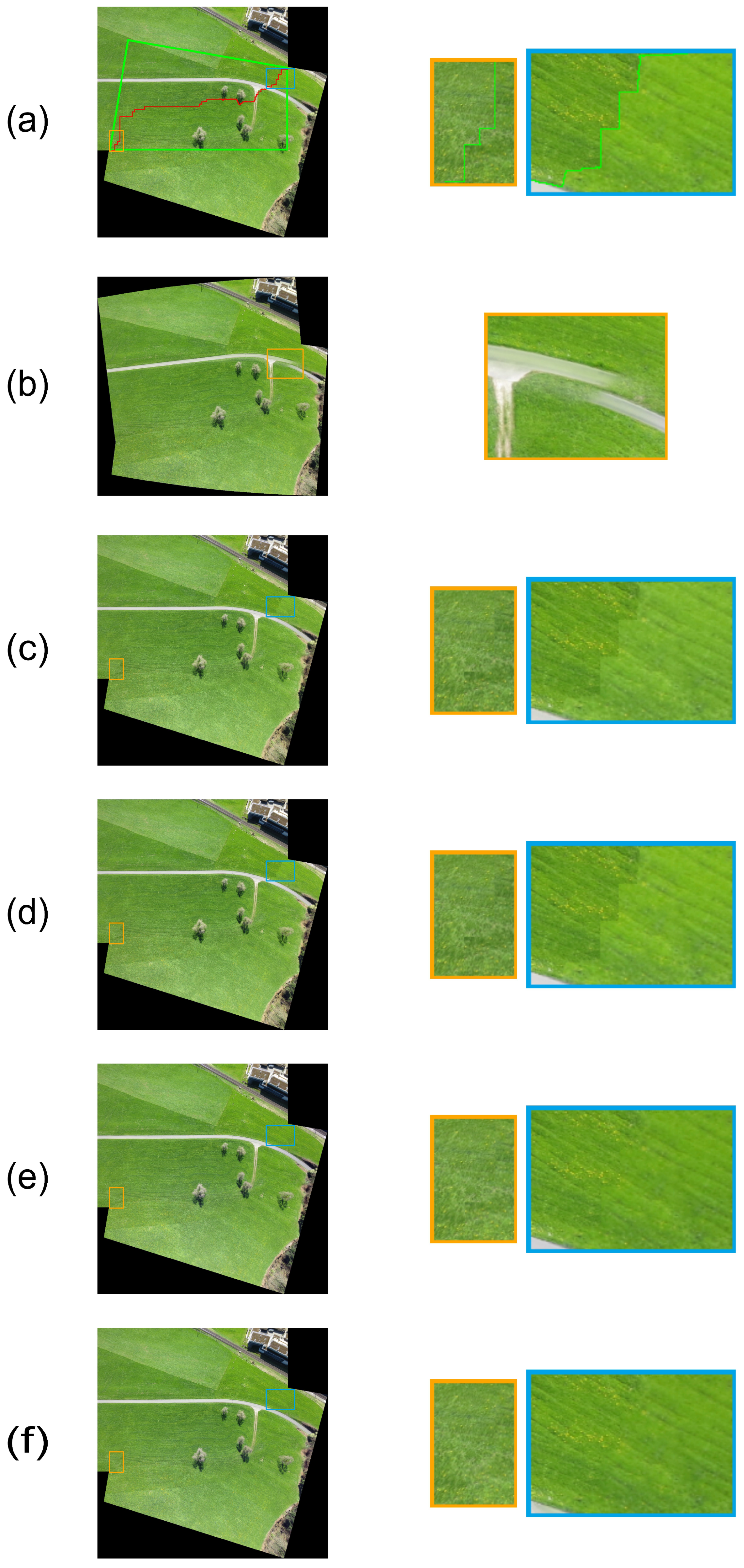
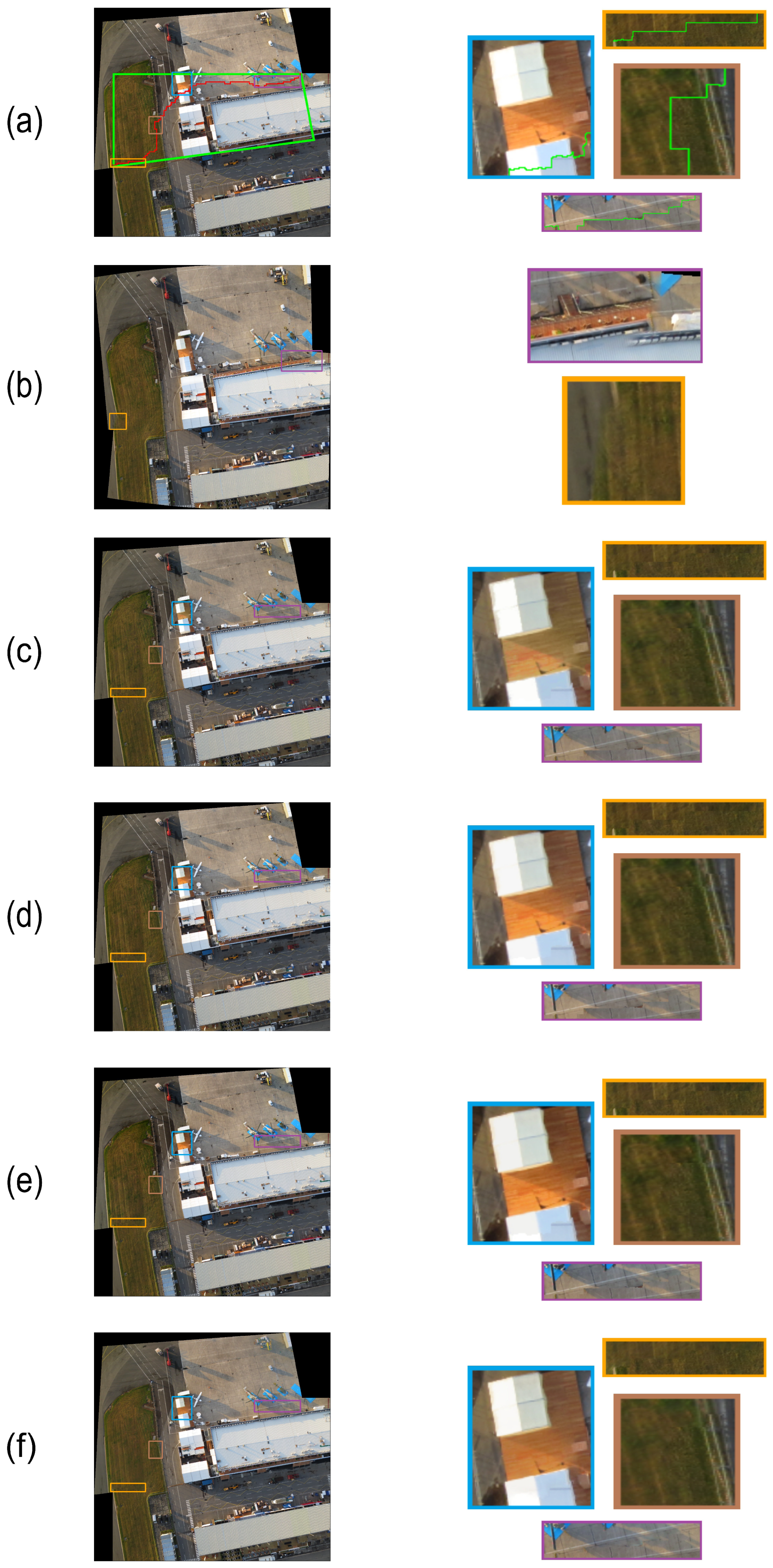
Five testing UAV stitched images under different misalignment and brightness situations are used to demonstrate the perceptual merit of the proposed ABJI-based method relative to the four comparative methods. For one testing stitched image, some amplified sub-images near the stitching line are adopted to justify the perceptual merit of our method.
The first testing UAV stitched image, which is taken from the set S 0 , is illustrated in Figure 8a. After performing the five considered methods on Figure 8a, Figure 8b–f shows the color correction results by using the MBB method, the HM-based method, the GP-based method, the GBJI-based method, and our method, respectively. It is notable that for the MBB method, the experimental demonstration is based on the tool that is downloaded from http://www.autostitch.net/ (accessed on 23 October 2021), so it is different from the other color correction methods. From Figure 8b–f, we observe that our method achieves the best perceptual gradation effect near the misaligned stitching target pixels, but for the four comparative methods, there are unsmooth artifacts. Our method also preserves a good color correction effect in the other areas.
The second, third, fourth, and fifth testing stitched UAV images are illustrated in Figure 9a, Figure 10a, Figure 11a, and Figure 12a, respectively, which are taken from S 1 under −15% brightness update, S 1 under +15% brightness update, S 2 under −25% brightness update, and S 2 under +25% brightness update. After performing the five considered methods on the four testing stitched images, Figure 9b–f, Figure 10b–f, Figure 11b–f and Figure 12b–f demonstrate the corresponding color correction results for Figure 9a, Figure 10a, Figure 11a, Figure 12a, respectively.
Figure 9b–f indicate that inside the three amplified sub-images, our method still achieves the best perceptual gradation effect near the misaligned stitching target pixels, but for the four comparative methods, there are some unsmooth artifacts. In Figure 10b–f, we observe that inside the two amplified grassland sub-images, our method achieves a more natural effect. For Figure 11b–f and Figure 12b–f, we have the same conclusion that, inside the amplified sub-images, our method achieves a more smooth effect near the misaligned stitching target pixels relative to the four comparative methods.
The main reasons for the quality superiority of the proposed color correction method are summarized as follows. Based on the two partitioned classes of the stitching color difference values, which are determined by the proposed split-and-merge approach, for each target pixel in Ω t , the suitable reference interval of the stitching color difference values is determined by the proposed wavefront approach. Finally, using this useful reference interval information, the proposed AJBI-based color blending method can achieve more natural and smooth color blending effects near the misaligned stitching target pixels. After running the five considered methods on the 40 testing stitched images, the 200 (5 × 40) color corrected stitched images can be accessed from the website in Supplementary Material. Interested readers can refer to these color correction results for more detailed perceptual quality comparison.

4.2. Computation of Time Cost

Based on the above-mentioned three testing sets, S 0 , S 1 , and S 2 , under different alignment and brightness situations, the last column of Table 1 tabulates the average execution time required by each considered color blending method for one testing stitched image in each testing set. We have the following two observations: (1) Among the five considered methods, the HM-based method [19] and the GP-based method [21] are the two fastest methods and (2) the execution time improvement ratio of the proposed ABJI-based method over the GBJI-based method [23] equals 13.52% ( 1 3 ( ( 3.5485 3.0975 ) + ( 3.5683 3.0881 ) + ( 3.6 3.0823 ) ) .
Although our method is not the fastest, it achieves the best perceptual quality performance, particularly near the misaligned stitching target pixels, and has the best objective quality performance among all considered methods.

5. Conclusions and Future Work

We have presented the proposed AJBI-based color blending method for stitched UAV images. First, the proposed split-and-merge approach partitions all stitching color difference values on the stitching line into two classes, namely the aligned class and the misaligned class. Next, based on the two partitioned classes of the stitching color difference values, a wavefront approach is proposed to determine a suitable reference interval of the stitching color difference values for each target pixel. Finally, using the useful reference information, the proposed AJBI-based color blending method can achieve better objective and subjective color blending effects. Based on 40 testing stitched UAV images under different misalignment and brightness situations, in terms of PSNR, SSIM, FSIM, and perceptual effects, the comprehensive experimental results have justified the robust objective and subjective quality benefits of our color blending method when compared with the four comparative methods [18,19,21,23].
Our future work will apply a window-based Gabor filter approach, to extract the textural feature of each stitching pixel on the stitching line, and then improve the current split-and-merge approach to better partition the stitching color difference values. Besides, it is a challenging problem to improve the proposed color blending method for each target pixel by fusing the corrected color, which is obtained by utilizing the determined reference interval of the stitching color difference values and the corrected color, which is obtained by using the state-of-the-art method, such as the HM-based method [19]. It is another challenging problem to develop methods to automatically determine the concerned thresholds, such as T c o s t , c, and c m i n , used in the proposed color blending method.

Supplementary Materials

The following supporting information can be downloaded at: https://github.com/Luzzzzzhe118/AJBI-based-_color_blending.

Author Contributions

Data curation, D.-Y.R.; Methodology, K.-L.C.; Project administration, K.-L.C.; Software, D.-Y.R.; Supervision, K.-L.C.; Validation, D.-Y.R.; Visualization, D.-Y.R.; Writing—original draft, K.-L.C.; Writing—review & editing, K.-L.C. All authors have read and agreed to the published version of the manuscript.

Funding

This work was supported by the contract MOST-111-2221-E-011-126-MY3 of the Ministry of Science and Technology, Taiwan.

Data Availability Statement

All datasets were obtained from the senseFly platform (https://www.sensefly.com/education/datasets/?dataset=1419, accessed on 6 April 2022).

Acknowledgments

We appreciate the proofreading help of C. Harrington and the comments provided by the three reviewers to improve the manuscript.

Conflicts of Interest

The authors declare no conflict of interest.

Appendix A. The Proof of Theorem 1

Theorem 1 is proved by the following derivation:
Proof. 
σ C a 2 = 1 n x C a ( x μ C a ) 2 = 1 n [ x C a ( x μ C a ) 2 + x C m ( x μ C a ) 2 ] = 1 n [ x C a ( x 2 2 x μ C a + μ C a 2 ) + x C m ( x 2 2 x μ C a + μ C a 2 ) ] = 1 n [ { | C a | ( σ C a 2 + μ C a 2 ) 2 | C a | μ C a μ C a + | C a | μ C a 2 } + { | C m | ( σ C m 2 + μ C m 2 ) 2 | C m | μ C m μ C a + | C m | μ C a 2 } ] = 1 n [ | C a | σ C a 2 + | C a | ( μ C a μ C a ) 2 ] + [ | C m | σ C m 2 + | C m | ( μ C m μ C a ) 2 ] = | C a | n σ C a 2 + | C m | n σ C m 2 + [ | C a | n ( | C m | μ C a | C m | μ C m n ) 2 ] + [ | C m | n ( | C a | μ C m | C a | μ C a n ) 2 ] = | C a | n σ C a 2 + | C m | n σ C m 2 + | C a | | C m | n 2 ( μ C a μ C m ) 2 = w a σ C a 2 + w m σ C m 2 + | C a | | C m | n 2 ( μ C a μ C m ) 2
We complete the proof. □

References

  1. Ezequiel, C.A.F.; Cua, M.; Libatique, N.C.; Tangonan, G.L.; Alampay, R.; Labuguen, R.T.; Favila, C.M.; Honrado, J.L.E.; Caños, V.; Devaney, C.; et al. UAV Aerial Imaging Applications for Post-disaster Assessment, Environmental Management and Infrastructure Development. In Proceedings of the 2014 International Conference on Unmanned Aircraft Systems (ICUAS), Orlando, FL, USA, 27–30 May 2014; pp. 274–283. [Google Scholar] [CrossRef]
  2. Adams, S.; Friedland, C. A Survey of Unmanned Aerial Vehicle (UAV) Usage for Imagery Collection in Disaster Research and Management. In Proceedings of the 9th International Workshop on Remote Sensing for Disaster Response, Stanford, CA, USA, 15–16 September 2011. [Google Scholar]
  3. Ugliano, M.; Bianchi, L.; Bottino, A.; Allasia, W. Automatically Detecting Changes and Anomalies in Unmanned Aerial Vehicle Images. In Proceedings of the 2015 IEEE 1st International Forum on Research and Technologies for Society and Industry Leveraging a Better Tomorrow (RTSI), Turin, Italy, 16 September 2015; pp. 484–489. [Google Scholar] [CrossRef] [Green Version]
  4. Avola, D.; Cinque, L.; Foresti, G.L.; Martinel, N.; Pannone, D.; Piciarelli, C. A UAV Video Dataset for Mosaicking and Change Detection From Low-Altitude Flights. IEEE Trans. Syst. Man Cybern. Syst. 2020, 50, 2139–2149. [Google Scholar] [CrossRef] [Green Version]
  5. Pajares, G. Overview and Current Status of Remote Sensing Applications Based on Unmanned Aerial Vehicles (UAVs). Photogramm. Eng. Remote Sens. 2015, 81, 281–329. [Google Scholar] [CrossRef] [Green Version]
  6. Yuan, W.; Choi, D. UAV-Based Heating Requirement Determination for Frost Management in Apple Orchard. Remote Sens. 2021, 13, 273. [Google Scholar] [CrossRef]
  7. Gao, J.; Li, Y.; Chin, T.J.; Brown, M.S. Seam-Driven Image Stitching. In Proceedings of the Eurographics 2013–Short Papers, Girona, Spain, 6–10 May 2013; Otaduy, M.A., Sorkine, O., Eds.; pp. 45–48. [Google Scholar] [CrossRef]
  8. Lin, K.; Jiang, N.; Cheong, L.F.; Do, M.; Lu, J. SEAGULL: Seam-Guided Local Alignment for Parallax-Tolerant Image Stitching. In Proceedings of the Computer Vision–ECCV 2016; Leibe, B., Matas, J., Sebe, N., Welling, M., Eds.; Springer International Publishing: Cham, Switzerland, 2016; pp. 370–385. [Google Scholar]
  9. Li, L.; Yao, J.; Liu, Y.; Yuan, W.; Shi, S.; Yuan, S. Optimal Seamline Detection for Orthoimage Mosaicking by Combining Deep Convolutional Neural Network and Graph Cuts. Remote Sens. 2017, 9, 701. [Google Scholar] [CrossRef] [Green Version]
  10. Yuan, Y.; Fang, F.; Zhang, G. Superpixel-Based Seamless Image Stitching for UAV Images. IEEE Trans. Geosci. Remote Sens. 2021, 59, 1565–1576. [Google Scholar] [CrossRef]
  11. Chen, J.; Li, Z.; Peng, C.; Wang, Y.; Gong, W. UAV Image Stitching Based on Optimal Seam and Half-Projective Warp. Remote Sens. 2022, 14, 1068. [Google Scholar] [CrossRef]
  12. Yin, H.; Li, Y.; Shi, J.; Jiang, J.; Li, L.; Yao, J. Optimizing Local Alignment along the Seamline for Parallax-Tolerant Orthoimage Mosaicking. Remote Sens. 2022, 14, 3271. [Google Scholar] [CrossRef]
  13. Lowe, D. Object Recognition from Local Scale-invariant Features. In Proceedings of the Seventh IEEE International Conference on Computer Vision, Kerkyra, Greece, 20–27 September 1999; Volume 2, pp. 1150–1157. [Google Scholar] [CrossRef]
  14. Dubrofsky, E. Homography Estimation. Ph.D. Thesis, University of British Columbia (Vancouver), Kelowna, BC, Canada, March 2009. [Google Scholar]
  15. Fischler, M.A.; Bolles, R.C. Random Sample Consensus: A Paradigm for Model Fitting with Applications to Image Analysis and Automated Cartography. Commun. ACM 1981, 24, 381–395. [Google Scholar] [CrossRef]
  16. Wang, G.; Chen, Y. Robust Feature Matching Using Guided Local Outlier Factor. Pattern Recognit. 2021, 117, 107986. [Google Scholar] [CrossRef]
  17. Liu, H.; Yin, S.; Sui, H.; Yang, Q.; Lei, D.; Yang, W. Accurate Matching of Invariant Features Derived from Irregular Curves. Remote Sens. 2022, 14, 1198. [Google Scholar] [CrossRef]
  18. Brown, M.; Lowe, D.G. Automatic Panoramic Image Stitching Using Invariant Features. Int. J. Comput. Vis. 2007, 74, 59–73. [Google Scholar] [CrossRef] [Green Version]
  19. Fecker, U.; Barkowsky, M.; Kaup, A. Histogram-Based Prefiltering for Luminance and Chrominance Compensation of Multiview Video. IEEE Trans. Circuits Syst. Video Technol. 2008, 18, 1258–1267. [Google Scholar] [CrossRef]
  20. Xiong, Y.; Pulli, K. Color Matching for High-quality Panoramic Images on Mobile Phones. IEEE Trans. Consum. Electron. 2010, 56, 2592–2600. [Google Scholar] [CrossRef]
  21. Xia, M.; Yao, J.; Gao, Z. A Closed-form Solution for Multi-view Color Correction with Gradient Preservation. ISPRS J. Photogramm. Remote Sens. 2019, 157, 188–200. [Google Scholar] [CrossRef]
  22. Yang, J.; Liu, L.; Xu, J.; Wang, Y.; Deng, F. Efficient Global Color Correction for Large-scale Multiple-view Images in Three-dimensional Reconstruction. ISPRS J. Photogramm. Remote Sens. 2021, 173, 209–220. [Google Scholar] [CrossRef]
  23. Fang, F.; Wang, T.; Fang, Y.; Zhang, G. Fast Color Blending for Seamless Image Stitching. IEEE Geosci. Remote Sens. Lett. 2019, 16, 1115–1119. [Google Scholar] [CrossRef]
  24. Li, L.; Xia, M.; Liu, C.; Li, L.; Wang, H.; Yao, J. Jointly optimizing global and local color consistency for multiple image mosaicking. ISPRS J. Photogramm. Remote Sens. 2020, 170, 45–56. [Google Scholar] [CrossRef]
  25. Li, Y.; Li, L.; Yao, J.; Xia, M.; Wang, H. Contrast-Aware Color Consistency Correction for Multiple Images. IEEE J. Sel. Top. Appl. Earth Obs. Remote Sens. 2022, 15, 4941–4955. [Google Scholar] [CrossRef]
  26. Cui, H.; Zhang, G.; Wang, T.Y.; Li, X.; Qi, J. Combined Model Color-Correction Method Utilizing External Low-Frequency Reference Signals for Large-Scale Optical Satellite Image Mosaics. IEEE Trans. Geosci. Remote Sens. 2021, 59, 4993–5007. [Google Scholar] [CrossRef]
  27. Wang, Z.; Bovik, A.; Sheikh, H.; Simoncelli, E. Image Quality Assessment: From Error Visibility to Structural Similarity. IEEE Trans. Image Process. 2004, 13, 600–612. [Google Scholar] [CrossRef] [Green Version]
  28. Zhang, L.; Zhang, L.; Mou, X.; Zhang, D. FSIM: A Feature Similarity Index for Image Quality Assessment. IEEE Trans. Image Process. 2011, 20, 2378–2386. [Google Scholar] [CrossRef] [PubMed] [Green Version]
  29. Lloyd, S. Least Squares Quantization in PCM. IEEE Trans. Inf. Theory 1982, 28, 129–137. [Google Scholar] [CrossRef]
  30. Cormen, T.H.; Leiserson, C.E.; Rivest, R.L.; Stein, C. Introduction to Algorithms, 3rd ed.; The MIT Press: Cambridge, MA, USA, 2009. [Google Scholar]
Figure 1. One stitching line example obtained by the method of Yuan et al. [10]. (a) The input source image I s and the target image I t . (b) The stitching line is marked in red and the overlapping area of I s and I t is surrounded by a green quadrilateral.
Remotesensing 14 05440 g001
Figure 2. The distributions of the absolute stitching c-color, c ∈ {R, G, B}, difference values of Figure 1b. (a) For R-color. (b) For G-color. (c) For B-color.
Remotesensing 14 05440 g002
Figure 3. The flowchart of the proposed split-and-merge approach.
Remotesensing 14 05440 g003
Figure 4. Partitioning each distribution of the absolute stitching c-color, c ∈ {R, G, B}, difference values in Figure 2 into two classes. (a) For R-color. (b) For G-color. (c) For B-color.
Remotesensing 14 05440 g004
Figure 5. The partition result of Figure 1b, where the aligned color difference pixels are marked in green color and the misaligned color difference pixels are marked in red color.
Remotesensing 14 05440 g005
Figure 6. Constructing all wavefronts for target pixels in Ω t .
Remotesensing 14 05440 g006
Figure 7. One updated stitched image and the partitioned stitching color difference values. (a) The original stitched image. (b) The updated stitched image by increasing 15% of the brightness of every target pixel in (a). (c) The partitioned stitching color difference values.
Remotesensing 14 05440 g007
Figure 8. The perceptual quality merit of our method for the first testing stitched image taken from S 0 . (a) The testing stitched image and the amplified sub-images near the stitching line. (b) The MBB method [18]. (c) The HM-based method [19]. (d) The GP-based method [21]. (e) The GBJI-based method [23]. (f) Our method.
Remotesensing 14 05440 g008
Figure 9. The perceptual quality merit of our method for the second testing stitched image taken from S 1 under −15% brightness update. (a) The testing stitched image and the amplified sub-images near the stitching line. (b) The MBB method [18]. (c) The HM-based method [19]. (d) The GP-based method [21]. (e) The GBJI-based method [23]. (f) Our method.
Remotesensing 14 05440 g009
Figure 10. The perceptual quality merit of our method for the third testing stitched image taken from S 1 under +15% brightness update. (a) The testing stitched image and the amplified sub-images near the stitching line. (b) The MBB method [18]. (c) The HM-based method [19]. (d) The GP-based method [21]. (e) The GBJI-based method [23]. (f) Our method.
Remotesensing 14 05440 g010
Figure 11. The perceptual quality merit of our method for the fourth testing stitched image taken from S 2 under −25% brightness update. (a) The testing stitched image and the amplified sub-images near the stitching line. (b) The MBB method [18]. (c) The HM-based method [19]. (d) The GP-based method [21]. (e) The GBJI-based method [23]. (f) Our method.
Remotesensing 14 05440 g011
Figure 12. The perceptual quality merit of our method for the fifth testing stitched image taken from S 2 under +25% brightness update. (a) The testing stitched image and the amplified sub-images near the stitching line. (b) The MBB method [18]. (c) The HM-based method [19]. (d) The GP-based method [21]. (e) The GBJI-based method [23]. (f) Our method.
Remotesensing 14 05440 g012
Table 1. The objective quality comparison.
MethodTesting SetPSNR (dB)SSIMFSIMTime (sec)
MBB [18] S 0 ---2.0804
HM [19] S 0 22.720.8580.7050.1821
GP [21] S 0 22.540.8570.7130.5533
GBJI [23] S 0 22.700.8590.7243.5485
Ours S 0 23.010.8600.7273.0975
MBB [18] S 1 ---2.0891
HM [19] S 1 22.700.8570.7040.1801
GP [21] S 1 22.450.8550.7120.5465
GBJI [23] S 1 22.580.8560.7253.5683
Ours S 1 22.910.8590.7283.0881
MBB [18] S 2 ---2.119
HM [19] S 2 22.650.8560.7030.1826
GP [21] S 2 22.210.8510.7120.545
GBJI [23] S 2 22.360.8520.7253.600
Ours S 2 22.710.8550.7283.0823
Publisher’s Note: MDPI stays neutral with regard to jurisdictional claims in published maps and institutional affiliations.

