Abstract
Quantifying vegetation responses after natural disasters helps clarify complex relationships between vegetation and surface processes such as soil erosion. The heterogenous post-disaster landscape offers a naturally stratified environment for this study. Existing research tends to be frequently monitored but small-scale or sporadically monitored but large-scale. The availability of high-quality and free satellite imagery bridges this gap by offering continuous, longer-term observations at the landscape scale. Here we take advantage of a dense Landsat time series to investigate landscape-scale vegetation response rates and factors at Unzen volcano, Japan. We do this by first investigating differences between two popular vegetation indices—The Normalized Difference Vegetation Index (NDVI) and the Normalized Burn Ratio (NBR), when applied to recovery studies. We then apply pixel-wise regressions to quantify spatio-temporal vegetation response and regression tree analyses to investigate drivers of recovery. Our findings showed that simple linear-log functions best model recovery rates reflecting primary succession trajectories caused by extreme disturbance and damage. Regression tree analyses showed that despite secondary disturbances, vegetation recovery in both the short and long-term is still dominated by eruption disturbance type and elevation. Finally, compared to NDVI, NBR is a better indicator of structural vegetation regrowth for the early years of revegetation.
Keywords:
Landsat; revegetation; landscape disturbance; vegetation indices; GIS; Unzen volcano; topography 1. Introduction
Interactions between ecological and geomorphological processes are highly complex, occurring at various spatial scales, landscapes, and on different timelines [1,2,3,4]. Many studies have hypothesized that such interactions can shape landscapes [5,6] and alter ecological systems [7,8] and are consequently very significant considering increased human influence [3] and changing climate [9]. However, traditional fields of ecology and geomorphology have tended to work separately, considering interactions only in one direction [7,10], and leaving out important feedbacks and dependencies [11]. For example, vegetation root reinforcement is affected by topography [12,13] and is itself a factor of slope stability [14]. Moreover, many studies on ecology–geomorphology interactions tend to focus on mature landscapes where interactions are mostly stable, and feedback loops have become more apparent [15]. Therefore, there is a need to study more dynamic landscapes at the initial stages of ecosystem and vegetation development and featuring early-stage ecology–geomorphological interactions [15,16]. Such ecosystems tend to feature complex non-linear relationships with threshold tipping points as they remain far from equilibrium [7,9,15].
However, there is a lack of early-stage ecology–geomorphology studies due to the difficulties in obtaining necessary data such as quantifiable early vegetation responses. Landscapes at initial stages of development are rare, for example, only developing after significant disturbances such as volcanic eruptions that wipe out previously existing biota [8,17] and transform ecosystems to an “initial” stage, featuring dynamic environments at disequilibrium [15]. In volcanic areas, eruption products can result in significant spatial heterogeneity across the landscape, forming natural experiments for examining long- and short-term vegetation recovery trends [8,16]. Post-eruption vegetation recovery and succession on volcanic slopes also depend on numerous factors, such as climate, surface heterogeneity, and distance from surviving vegetation [8]. In addition, stochastic elements can disrupt expected succession pathways, leading to uncertain recovery and succession mechanisms [18]. Unfortunately, obtaining field access to post-eruption landscapes is often time-sensitive, dangerous, and expensive. Nevertheless, dynamic data on vegetation recovery rates and patterns are necessary to comprehensively understand the feedbacks in ecology–geomorphology interactions [7]. Some studies have investigated vegetation recovery after volcanic eruptions, for example, at Mount St. Helens, USA [17], Pinatubo, the Philippines [19], Mount Usu, Japan [20], and Unzen volcano, Japan [21]. However, volcanic revegetation has primarily been studied at the small-scale using plot-based analyses [21,22] or at the landscape scale using sparse remote sensing data [19,23].
In this respect, longer-term remote sensing data collections such as the Landsat dataset provide an unparalleled opportunity to safely study short- and long-term landscape-scale vegetation recovery. Landsat satellites provide historical data from the 1980s, unlocking remote access to historical eruptions and corresponding vegetation responses. To track vegetation recovery with remote sensing and Landsat, vegetation indices are used as a proxy [14,24]. Many indices are derived from mathematical operations on different spectral bands of multispectral imagery. However, vegetation index response depends on disturbance type [25], the measured vegetation characteristic [26], soil and vegetation type [27,28,29], and the presence of other background materials such as charcoal [30]. Either both background and vegetation variability or one of them can significantly change vegetation index response, greatly increase uncertainties, and cause anomalies [27,30,31]. Consequently, many studies have discussed the appropriateness of different vegetation indices given the numerous confounding factors [32,33].
Considering the Landsat spectral resolution and the available spectral bands, the Normalized Difference Vegetation Index (NDVI) [34] and the Normalized Burn Ratio (NBR) [35] are two of the commonly used vegetation indices for vegetation mapping, recovery, and disturbance studies. NDVI is widely used because it has been shown to provide reasonable estimates of vegetation cover for different vegetation types [36] and across different soil and lithological backgrounds [30,37], due to its normalizing capability that minimizes the impact of background variations [27]. NDVI has been positively correlated to the leaf area index (LAI) and biomass [38], but the sensitivity of this relationship decreases past a certain threshold or amount of vegetation cover [39]. NBR was initially developed as an index to measure and map burn severity, i.e., the magnitude of ecological change caused by fire [35], but has recently been used to track and characterize forest recovery over time, since studies have found that NBR’s mid-infrared wavelengths can be related to structural components of vegetation [33,40,41], although it also faces similar uncertainties with vegetation and soil variabilities [30].
With increasing amounts and frequency of remote sensing data and improved computing platforms to handle large datasets, new opportunities to understand landscape-scale vegetation response at post-disturbance sites are now available. Therefore, this study uses these advantages to investigate the spatial and temporal variations of vegetation recovery at a post-eruption site: Unzen volcano in Japan. To achieve this aim, there are three research objectives. First, to test the potential of using NBR against NDVI for improving quantification of vegetation recovery. Second, to use dense satellite images to quantify revegetation rates and patterns using the appropriate vegetation indices. Finally, to clarify if factors of volcanic revegetation can be investigated deterministically by using regression tree analyses to evaluate relationships between vegetation recovery rates and biogeographical factors such as topography and existing vegetation in light of secondary disturbances.
2. Materials and Methods
2.1. Study Site
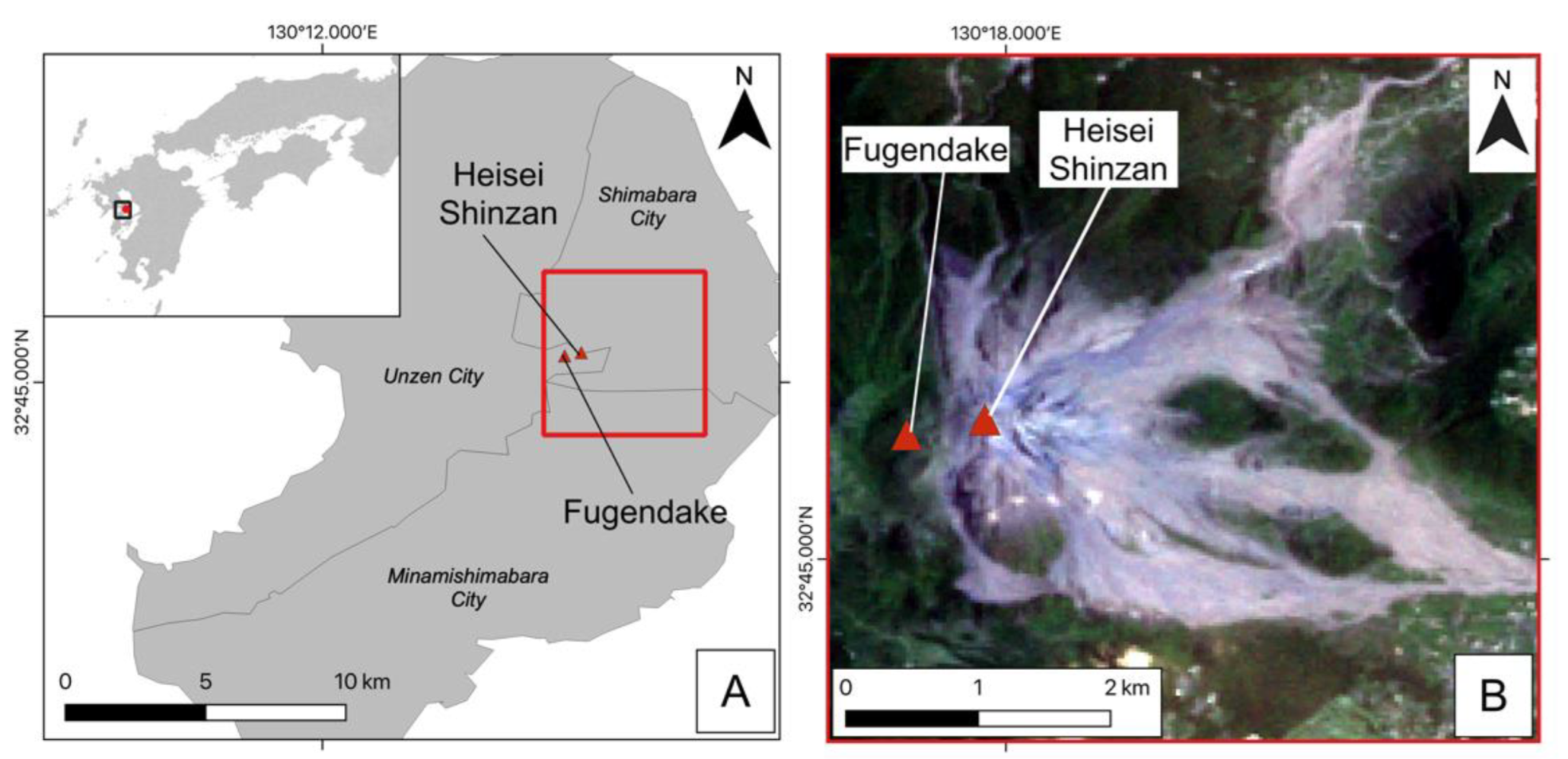
Unzen volcano is an active composite volcano located on the Shimabara Peninsula in Nagasaki Prefecture, Kyushu, Japan (Figure 1). It experiences a humid subtropical climate featuring hot summers with heavy rainfall and cold but mild winters [42]. Vegetation zones can be approximately divided into an evergreen forest zone above 1000 m and a deciduous forest zone below 1000 m [43]. After 198 years of dormancy, Unzen volcano erupted in November 1990, beginning an eruption sequence that ended in February 1995 [44]. The eruption period generated multiple pyroclastic flows, mostly over the eastern flank of Fugendake (Figure 1), one of Unzen volcano’s peaks, resulting in the loss of lives and infrastructure, and changes to vegetation and topography [45]. Pre-eruption vegetation in the study area comprised a mix of coniferous evergreen and deciduous trees such as pine, maple and Japanese cedar, as well as grasses and shrubs such as the Kyushu azalea and silver grass [46]. During the eruption, pyroclastic flows and tephra falls damaged and destroyed much of the vegetation on Fugendake’s eastern slopes, leaving a great swath of bare land. By the eruption’s end, the original landscape of eroded andesite and dacite lava, and pyroclastic flow deposits [45] had been overlain and altered by more heterogenous deposits of fine-grained ash-fall, lahars, dead and blown-down trees, and poorly sorted pyroclastic flow deposits, amongst others [44,47]. In addition, slow and continuous lava effusion formed a lava dome complex near the Fugendake summit, now named Heisei Shinzan (Figure 1; [44]). The volcanic deposit thickness decreased with increasing distance from Heisei Shinzan [48] and lahars had occurred multiple times due to debris remobilization from rainfall during the summer rainy seasons of the eruption period [44]. Consequently, artificial revegetation activities, one of the most extensive in Japan [49], were undertaken to reduce erosion rates after the eruption had ceased [21]. Aerial seeding and reforestation conducted by the Kyushu Regional Forest Office and the Shimabara Branch Office of the Nagasaki Prefectural Government sporadically from 1996 to 2002 distributed more than 15 different seeds of native and non-native herbs and grasses [50] such as Japanese pampas grass and false indigo, and trees such as Alders and black pine across most of the damaged area [49,51].

Figure 1.
The Unzen volcano study site. (A): Location of the site (smaller red box) on the Shimabara Peninsula (grey on the main map). The inset map shows the location of the Shimabara Peninsula (black box inside inset) in southwest Japan. (B): Results of 1990–1995 eruption at the site from an RGB Landsat image taken on 6 June 1995—A few months after the eruption had ceased. The Fugendake and Heisei Shinzan peaks are identified by red triangles in both (A,B).
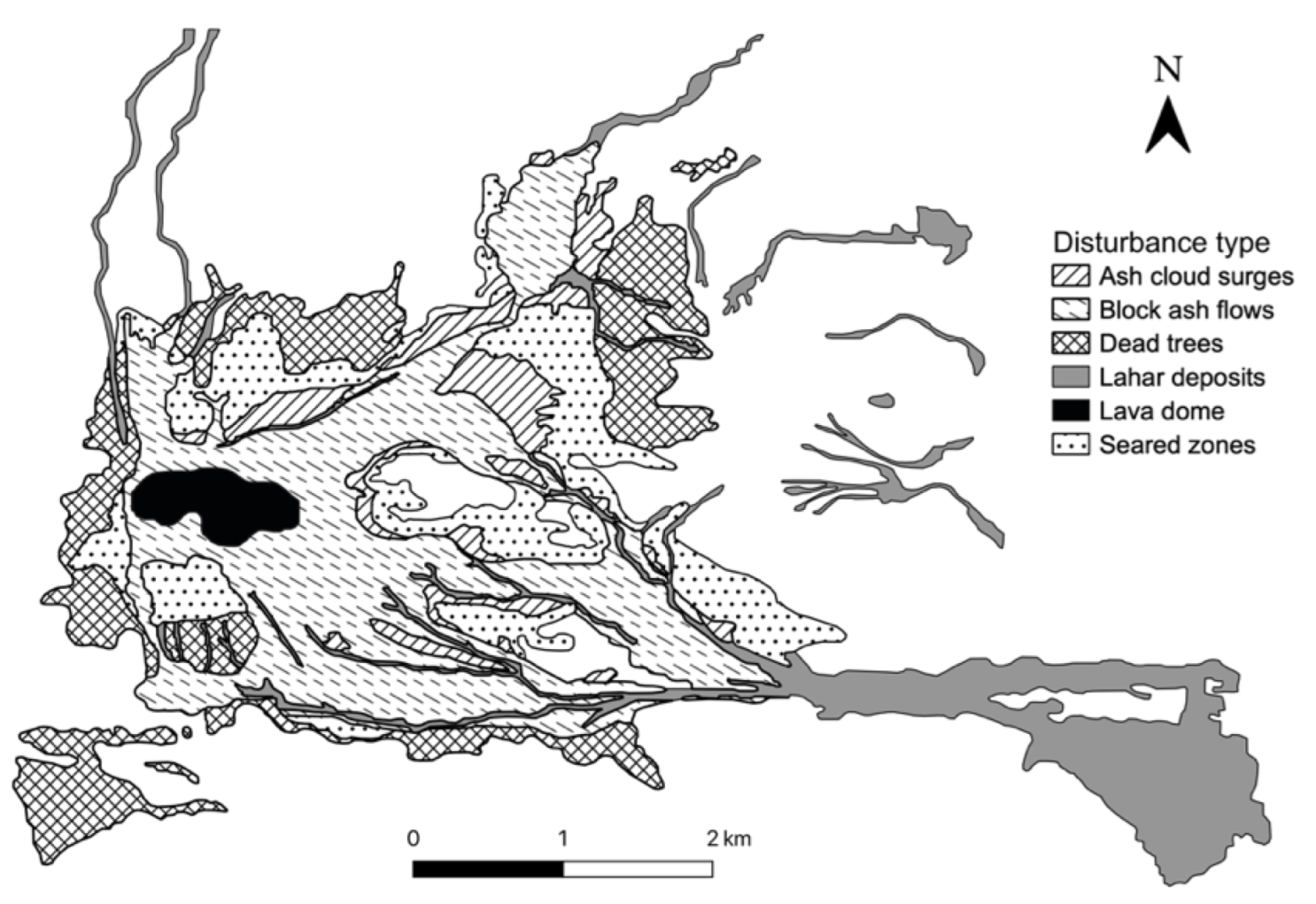
Unzen volcano was chosen as a study site due to the correspondences between the eruption period, the hypothesized vegetation recovery trends, and the data availability from Landsat images as well as previous studies on ground-truthed vegetation types and disturbance maps. Disturbance deposits were identified and mapped by [29] from aerial photographs taken a few months after the eruption ended. Therefore, to investigate post-eruption recovery, this study examined the entire approximately 20 km2 area at Unzen volcano affected by the eruption, which encompassed bare soil and mixtures of soil and vegetation at varying degrees of damage (Figure 1B and Figure 2). The bare soil surface has a mixture of volcanic ejecta, sandy soil and gravel, with very low water retention capacity [52]. In areas that have been vegetated over time, topsoil rich with humus was found due to the large amounts of organic matter supplied [53].
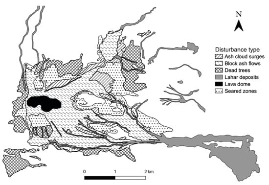
Figure 2.
Map of the 1990–1995 eruption deposits and disturbances, based on aerial photographs taken on 18 September 1995, adapted and digitized from [47].
2.2. Landsat Data and Pre-Processing
To derive annual NBR and NDVI time series from Landsat to track vegetation response, we first have to pre-process a dense stack of Landsat 5, 7, and 8 surface reflectance images. We downloaded Landsat images from Google Earth Engine, a cloud-computing platform capable of hosting and processing large amounts of satellite imagery [54], and conducted the following pre-processing steps through its Python API. Landsat surface reflectance images with a 30 m resolution have already been calibrated, converted to top-of-atmosphere reflectance, and atmospherically corrected [55], therefore better representing Earth’s surface and offering the image quality necessary for time series analyses. To obtain the necessary data, we filtered the entire surface reflectance dataset by the study site’s geographical boundary and for the months of June through September for the years 1984–2021. This period is considered long in remote-sensing terms and covers the pre- and post-eruption vegetation and the months for peak vegetation growth, which allows us to measure annual trends from a common baseline. For Landsat 7, we only accepted images from 1999–2002 due to the Scan Line Corrector failure error that occurred in 2003, which caused data gaps in images acquired after June 2003 [56]. We further filtered the data for the following parameters to ensure image quality: for cloud cover over land to be less than 80%, the geometric root mean squared error to be less than 10%, and the image quality to be greater than 7, where image quality refers to a USGS grading from 0 to 9, with 0 being the worst and 9 being the best composite quality image for all bands [57]. With the filtered dataset, we performed cloud masking using the Pixel Quality Assessment band and followed [58] to mask clouds out and reduce erroneous values. However, since sensor differences exist amongst Landsat 5, 7, and 8, to ensure consistency across the time series, images from different Landsat satellites have to be harmonized. While studies have suggested multiple harmonization methods, here we harmonized Landsat data using statistical functions that were developed using ordinary least-square regressions between data from thousands of near-simultaneous Landsat 7 and 8 images [59]. These statistical functions transform between different Landsat bands to ensure temporal continuity [59] and have been successfully used by other studies to derive consistent Landsat time series [60]. Finally, we classified the images by year and composited all image band values by the yearly median to obtain the dataset of median annual multispectral images for peak summer vegetation.
2.3. Deriving Explanatory Variables of Vegetation Recovery
To derive data on the driving factors of vegetation recovery for running regression analyses, we used QGIS to produce, calculate, and reproject multiple shapefile layers (Table 1) from various data sources. These formed the topographic, eruption, and geographic explanatory variables later used in regression tree analyses. All shapefiles were georeferenced to the coordinate system EPSG:2443 (JGD2000) for analyses.
Topographic variables of the slope, gradient, aspect, and profile curvature were calculated using the respective Geospatial Data Abstraction Library (GDAL) tools in the QGIS processing toolbox from a 5 m digital elevation model (DEM) produced in 2015 by the Geospatial Information Authority of Japan (GSI) and downloaded by us into QGIS. The resulting topographic shapefiles were resampled to 30 m resolution using the r.sample.interp tool to match Landsat spatial resolution. These topographic variables were chosen as studies show they affect vegetation growth. Slope gradient affects land stability and erosion rates, leading to changing probabilities of vegetation survival under deposits or in erosion-created gullies [23]. Aspect refers to the direction a slope faces, creating differences in solar insolation that affect ecological and geomorphological processes [61]. Elevation drives temperature and moisture levels, generating climate gradients as the elevation changes [62]. Profile curvature affects soil moisture distribution and seed transportation, thus affecting vegetation growth [63].
Eruption deposit types and extents had been previously mapped and identified [47]. To obtain an analyzable shapefile of these deposits, we georeferenced the existing map to an already-georeferenced Landsat image from the approximate same time period, and then digitized the map (Figure 2; Table 2). This processing was handled in QGIS.
Geographic data representing the ‘distance from surviving vegetation’ and ‘distance from crater’ variables were derived from the 5 m DEM and digitized map in QGIS. The distance from surviving vegetation was defined as the distance from a pixel within the disturbance zones of ‘block and ash flows’ or ‘lava dome’ to the nearest edge of those zones. Block and ash flows and lava dome disturbance types are considered primary disturbance types [8] and are known to almost wholly devastate all vegetation [64]. Therefore, we assume that within these areas, no vegetation has survived. The distances from surviving vegetation are consequently derived by first using the ‘Polygons to lines’ tool to convert the disturbance zone polygons to lines. Next, the QGIS Field Calculator was used to calculate the Euclidean distance between a pixel to the nearest line segment of the primary disturbance zones. The disturbance from crater variable was defined as the distance from a pixel of interest to the centroid of the lava dome area. This shapefile variable was calculated by first determining the centroid of the lava dome area, and then similarly calculating the Euclidean distance from a pixel to the centroid.

Table 1.
Summary of explanatory variables used for regression tree analyses. The value ranges are from our analysis of the explanatory variables in QGIS.
Table 1.
Summary of explanatory variables used for regression tree analyses. The value ranges are from our analysis of the explanatory variables in QGIS.
| Explanatory Variables | Value Range | Data Source |
|---|---|---|
| Disturbance type | Dead trees, lahar deposits, ash cloud surges, seared zones, block and ash flows, lava dome | [47] |
| Distance from surviving vegetation | 0.0–775.6 m | [47,64] |
| Distance from crater | 0.0–7013.0 m | [47] |
| Slope gradient | 0.1–69.0° | GSI Resampled 30-m DEM |
| Elevation | 6.7–1461.1 m | GSI Resampled 30-m DEM |
| Aspect | N, NE, E, SE, S, SW, W, NW | GSI Resampled 30-m DEM |
| Profile curvature | −0.045–0.042 | GSI Resampled 30-m DEM |

Table 2.
Description and statistics of disturbance types defined by [47]. The pixel count and area values are based on our computation using boundaries shown in Figure 2.
Table 2.
Description and statistics of disturbance types defined by [47]. The pixel count and area values are based on our computation using boundaries shown in Figure 2.
| Disturbance Type | Pixel Count | Area (% of Total) | Definition |
|---|---|---|---|
| Dead trees | 4563 | 20.32 | Areas of standing dead trees killed by volcanic gas and ash cloud |
| Lahar deposits | 3389 | 15.10 | Pyroclastic flow deposits that had been reworked and eroded |
| Ash cloud surges | 1673 | 7.45 | Areas covered by ash cloud deposits and blown-down trees |
| Seared zones | 4281 | 19.10 | Areas seared by ash clouds |
| Block and ash flows | 7963 | 35.45 | Areas directly impacted by the pyroclastic flow |
| Lava dome | 591 | 2.63 | Area of lava dome formation |
| Total area | 22,560 | 100 |
2.4. Computing and Comparing NDVI and NBR
From the pre-processed Landsat time series dataset, we calculated annual NDVI and NBR values and examined their spectral responses according to different disturbance types. Examining differences in vegetation index responses for each disturbance type can elucidate the ability of NDVI or NBR to capture biophysical changes resulting from different damage intensities. NDVI and NBR are calculated as follows:
where NIR is the near-infrared band, RED is the visible red band, and SWIR is the short-wave infrared band. Theoretical values of NDVI and NBR range from −1 to +1, where increasingly positive values represent healthier vegetation and negative and close-to-zero values are associated with bare soil [35], NIR is labelled as Band 4 for Landsat 5 and 7, and as Band 5 for Landsat 8. RED is labelled as Band 3 for Landsat 5 and 7, and as Band 4 for Landsat 8. SWIR is labelled Band 7 for Landsat 5 and 7, and as Band 7 for Landsat 8.
To compare NDVI and NBR results, Glass’s delta was used to test the differences in means. The large and different sample sizes and standard deviations of the datasets meant that typical statistical measures could not be used. Glass’s delta measures the effect size, or the magnitude of difference between two groups [48], and was therefore an appropriate test to determine the magnitude of changes between NBR and NDVI [65]. It is calculated as follows:
where is Glass’s delta, M1 and M2 are the means of two groups, and is the standard deviation of the first group (the control group). Glass’s delta values loosely define effect sizes as small ( 0.20), medium (0.50), and large (0.80) [66].
2.5. Deriving Vegetation Recovery Trends and Metrics
To investigate vegetation trends only from areas affected by the eruption, we need first to identify which pixels from the Landsat image are ‘disturbed’ [67]—i.e., affected by the eruption. The digitized map (Figure 2) was used as a Boolean mask to filter for affected pixels. To verify the validity of the digitized map, a separate threshold filter was applied to the original image stack, where the threshold filter identifies pixels that show a significant NBR value change pre- and post-eruption (greater than 20% of the pre-eruption value), following the threshold applied by [67]. Since pixels identified by the threshold filter as ‘disturbed’ were very similar to those identified by the digitized map, the digitized map was validated and used as a final filter. If pixels were not classified as ‘disturbed’, we excluded them from further analyses. In addition, if the time series data for a particular pixel had too few values (fewer than 19 valid measurements—i.e., half of the total possible number of measurements), we excluded the pixel to reduce any erroneous interpretations. With the resulting pixels, we performed pixel-wise regressions for the post-eruption time series data using a linear-log model:
where is the vegetation index value at time t, which is the number of years after the eruption, α is the constant corresponding to the intercept of the linear-log relationship, and β is the constant representing the slope of the relationship. Following trend analysis methods from previous post-eruption revegetation studies [19,23,68], we hypothesized that the recovery trend of our study area would follow similar logarithmic regrowth rates, where initial recovery rates will be faster than later recovery rates, given the relatively long 30-year period of our analyses. We also tested a simple linear model, but the fitting was much poorer. Equation (4) provides each pixel’s post-eruption recovery curve (Figure 3).
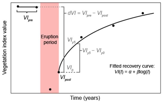
Figure 3.
Schematic illustration of a pixel’s time-series trajectory, its associated fitted linear-log curve, and variables derived for Equations (4)–(6). The red column indicates the eruption period.
In addition, we derived four recovery metrics from the recovery curve (Equation (4)) to more comprehensively characterize vegetation response. These recovery metrics were based on the previous studies that successfully characterized vegetation recovery after disturbances [23,33,40,69], and are later used as response variables for regression analyses. We only extracted metric values from pixels where the r2 and p-values of the fitted curve were greater than 0.7 and less than 0.05, respectively. This ensures that the extracted four metrics properly represent the time series data for that pixel.
The first metric is the years the pixel took to reach 80% of the pre-eruption vegetation index value (YEAR80), representing the long-term characterization [33]. The second metric is the years taken to reach 20% of the pre-eruption vegetation index value (YEAR20), representing the short-term characterization [23]. The third metric is the slope of the linear-log model (β), which describes how abruptly or gradually the recovery rate changes over time [23,67]. The fourth metric is the recovery indicator (RI), which is defined as a relative measure of post-disturbance regrowth [69] calculated as:
where the numerator is the difference in vegetation index values in the first five years after disturbance; VIy5 and VIy0 correspond to the vegetation index values derived from the fitted regression curve five years after disturbance and the year of disturbance, respectively (Figure 3). The denominator (dVI) refers to the difference between the immediate post-eruption vegetation index value (VIpost) and the pre-eruption vegetation index value (VIpre). This difference is defined as the disturbance magnitude (dVI):
where VIpost was obtained from averaging vegetation index values in the summer months of 1995, a few months after the eruption ceased in February 1995; VIpre was obtained by averaging vegetation index values from 1985 and 1986, as these pre-eruption years had the best quality images with the fewest pieces of missing data and assuming that vegetation cover from 1986–1990 was similar. Since vegetation recovery is affected by the disturbance magnitude, the RI metric scales recovery against disturbance magnitude, compensating for lower-magnitude disturbances [69]. Other studies have used the first five years for computing RI [40], and the same period was used in this study, given the trajectories observed by the vegetation recovery at Unzen volcano. Larger RI values indicate a higher recovery ratio to the disturbance magnitude.
2.6. Regression Tree and Correlation Analyses
To test the hypothesis that landscape-scale factors of volcanic revegetation can be explained deterministically, regression tree analysis (RTA) was used to model the effect of explanatory variables on vegetation recovery metrics. Regression trees are a form of decision trees that partition a data set into successively smaller subsets to predict the average response of that particular subset [70]. RTA results can identify the importance of explanatory variables to the response variable and the conditions under which the explanatory variable is important. RTA was chosen over other analytical regressions because the relationships between the explanatory and response variables are likely complex and nonlinear. Moreover, compared to machine learning-based models, RTA results are more interpretable for clarifying revegetation factors [23,71].
RTA was conducted for four recovery metrics, YEAR80, YEAR20, β and RI, respectively, using the rpart package [72] in R. This allows us to gain insights into the possible main drivers of long-term, short-term, and overall vegetation responses. To determine if all the explanatory variables from Table 1 should be included in RTA, Spearman’s rho statistic was calculated using the cor.test function of R to test for associations amongst the explanatory variables. Spearman’s rho was chosen due to the apparent nonlinear relationships between explanatory variables. While aerial seeding had occurred, it took place sporadically across almost the entire damage area at Unzen volcano, except for the lava dome area [21], and therefore was assumed to be a spatially uniform secondary disturbance at the landscape scale and not included in RTA.
However, one drawback of decision trees is their tendency to overfit the data if the trees are not ‘pruned’, i.e., cut back to minimize over-complexity but maximize accuracy [72]. To mitigate this, we conducted a grid search of optimal parameter values by creating multiple decision trees and identifying parameters to prune the tree and minimize the cross-validation error. The optimized parameters used for pruning are the minimum number of splits (minsplit), maximum depth (maxdepth), and cost-complexity value (cp). To verify these results, we checked the changes in relative error (1–R2), and cross-validation error as more splits were made. The optimal parameters should most significantly improve the fit with each split without increasing the cross-validation error. This resulted in four regression trees, one for each response variable.
3. Results
3.1. NDVI and NBR Spectral Responses
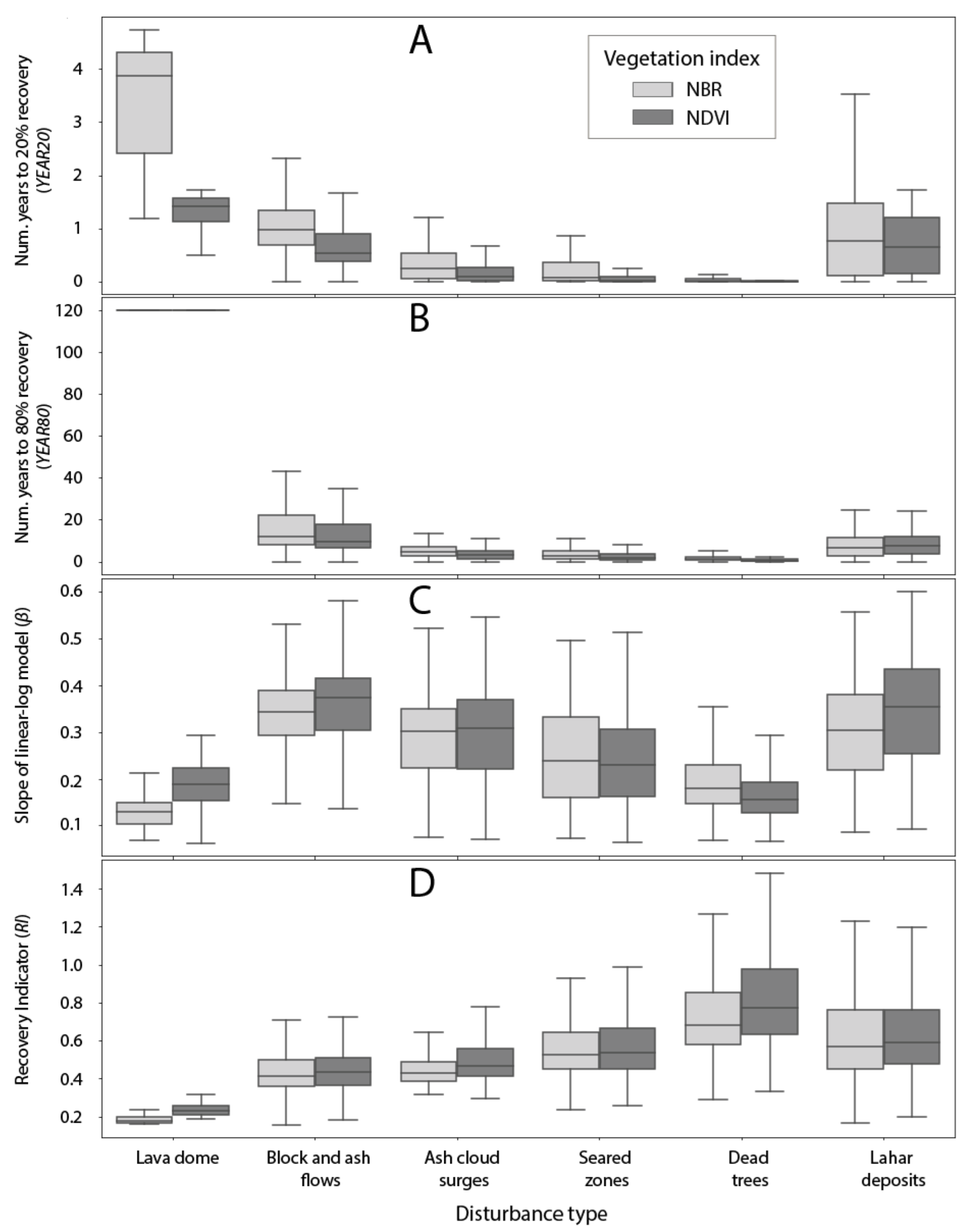
NDVI and NBR recovery metrics for each disturbance type were plotted in Figure 4, with outliers removed or modified. The outliers of β are those with negative values. YEAR80 outliers are values greater than 120, which were converted to 120. The duration of 120 years was chosen as the maximum cap for YEAR80 as it represents an ecologically possible outcome. YEAR20 and RI outliers are values less than or greater than the 2nd and 98th percentile, respectively. Outliers were defined by examining the results’ spatial distributions, ecologically-logical timelines, and histograms.
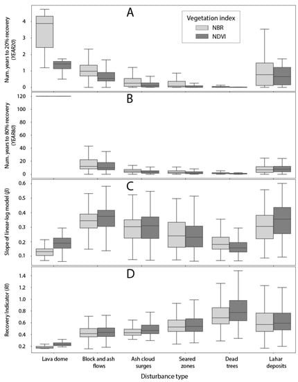
Figure 4.
Distribution of recovery metrics (y-axis) for each disturbance type (x-axis) and for each vegetation index (legend). (A): Number of years required to reach 20% of the pre-eruption vegetation index value (YEAR20); (B): Number of years to reach 80% of the pre-eruption vegetation index value (YEAR80); (C): Slope (β) of the linear-log model; (D): Recovery indicator value (RI).
For discriminating vegetation responses over time, Glass’s delta results show that the differences between NBR and NDVI lie primarily in areas where damage is the most intense—i.e., the lava dome area and block and ash flows, and in the early years of recovery (i.e., YEAR20) (Table 3). NBR indicated a mean of four years to reach 20% recovery, while NDVI indicated a mean value of 1.5 years. NBR also shows a larger range of values for YEAR20 results compared to NDVI. Due to outlier modification, NBR and NDVI both indicate a mean value of 120 years to reach 80% recovery, but an examination of the outliers showed that NDVI YEAR80 values were smaller than NBR YEAR80 values. From these results and as later discussed in Section 4, we conclude that NBR can better detect damage severity levels and is a clearer indication of vegetation recovery rates. Therefore, we focus only on NBR-derived responses in subsequent analyses.

Table 3.
Glass’s delta results, where results that indicate a large effect size (Δ ≥ 0.80) are in bold.
3.2. NBR Temporal Recovery Trends
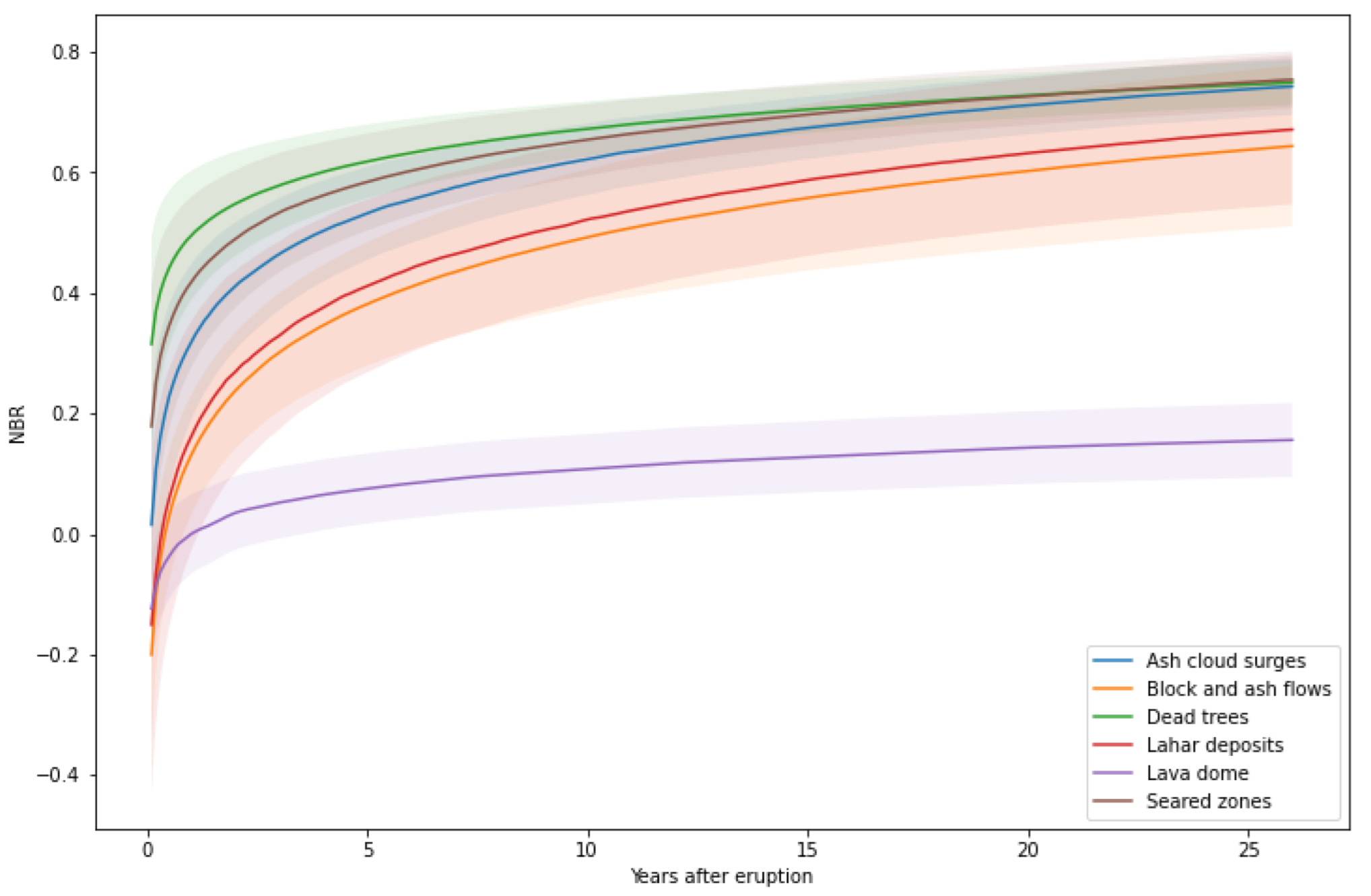
The time series NBR values showed a logarithmic recovery trend from the baseline post-eruption NBR value (Figure 5). The initial recovery rate for approximately the first five years is higher than that for the later years. Pixel-wise regression curves were averaged according to disturbance type, and their mean parameters are plotted in Figure 5, with one standard deviation represented. The linear-log model fit NBR responses well across all disturbance types and mainly differed in the absolute NBR value. Figure 5 also shows that the average regression curves can be approximately divided into three groups: (1) lava dome, (2) block and ash flows and lahar deposits, and (3) ash cloud surges, dead trees, and seared zones. Moreover, the linear-log model fits most of the pixels’ time-series data well, showing r2 values above 0.7 and p-values less than 0.05 (Figure 6A,B, respectively). The linear-log model showed a better fit (higher r2 values) for pixels closer to the middle of disturbed areas, as well as on the western and southern sides of the summit area (Figure 6A).

Figure 5.
Average recovery curves from each disturbance type with one standard deviation represented.
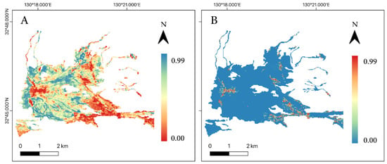
Figure 6.
Spatial distribution of r2 values (A) and p-values (B) from linear-log regression fitting. Note the color bar inversion in (B).
3.3. Spatial Variation of NBR-Derived Recovery Metrics
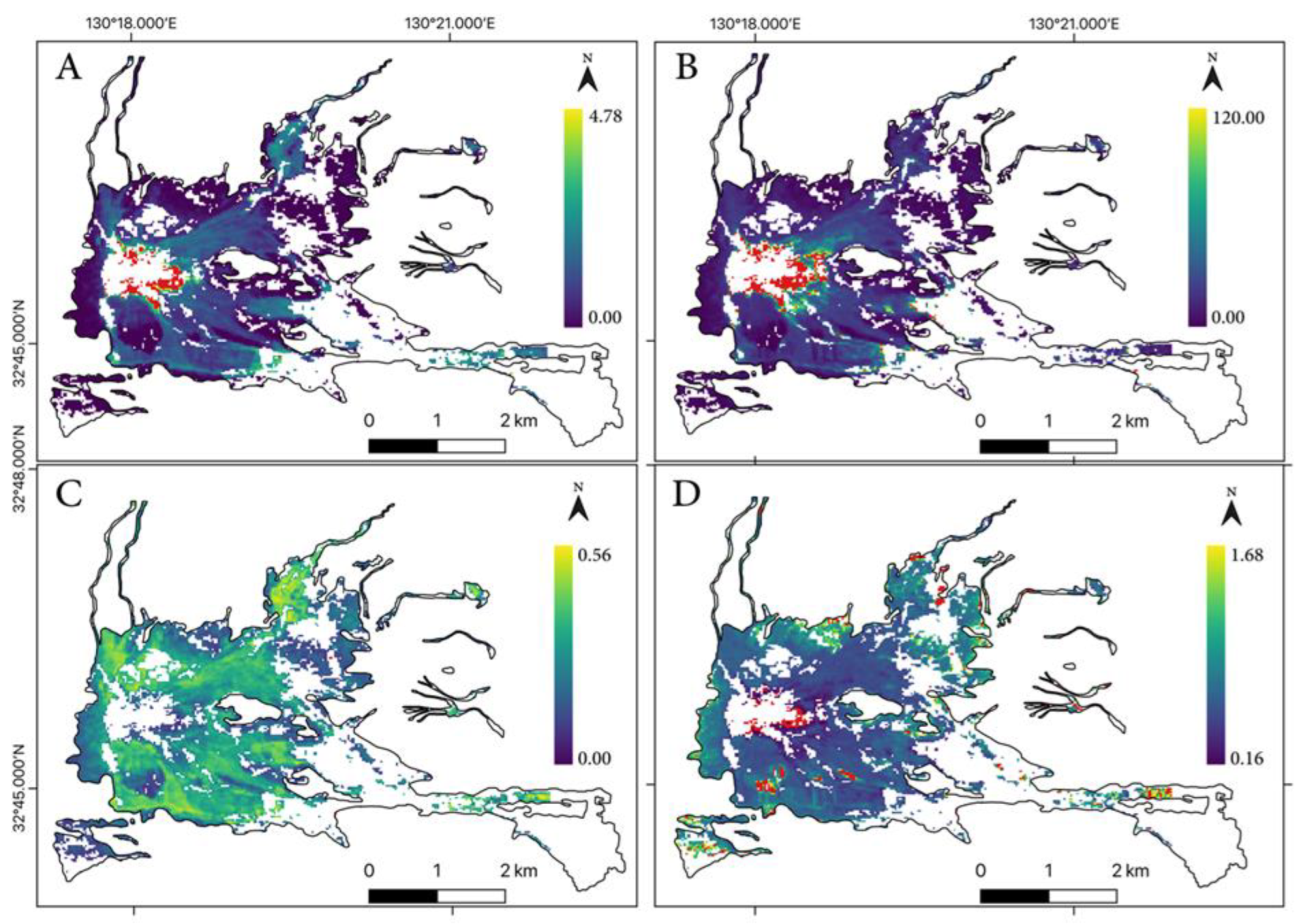
The spatial variations of the four recovery metrics are mapped in Figure 7. The maps identify the outliers respective to each recovery metric as red pixels. The short- and long-term spatial patterns of recovery appear similar (Figure 7A,B); the edges furthest from the crater show much quicker recovery rates, and recovery rates slow down towards the centers of affected zones and the crater. Sharp demarcations amongst short-term metric values are also present, for example, clear shapes and lines delineated between greenish pixels (higher YEAR20 values) and darker blue pixels (lower YEAR20 values). For β, a spatial variation similar to the long-term results is observed. Larger β values reflect a gentler curvature (slower changes in recovery times), while smaller values reflect a steeper curvature (quicker changes in recovery times). Higher positive values are generally observed towards the centers of the disturbed areas (Figure 7C). RI also shows a similar spatial variation to the other results, with higher RI values observed at the outermost edges of the disturbed areas (Figure 7D).
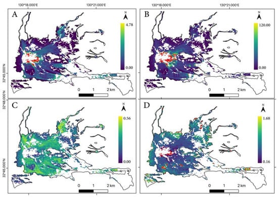
Figure 7.
Spatial distribution of response variables. (A): Number of years to 20% pre-eruption NBR (YEAR20); (B): Number of years to 80% pre-eruption NBR (YEAR80); (C): Slope (β) of the linear-log model; and (D): Recovery Indicator (RI). Red pixels represent outliers for each response variable. A thin, black border represents the disturbance zone boundary. Transparent pixels within the disturbance zone indicate pixels derived from poor-fitting regression curves and are not included.
3.4. Correlation Analysis and Regression Tree Results
Spearman’s rho statistic results showed that one of the explanatory variables (distance from crater) showed a high correlation (−0.903) to another variable (elevation) (Table 4). The former variable was therefore left out of the regression tree analyses.

Table 4.
Spearman’s correlation results from initial explanatory variables. DC: Distance from crater; DF: Distance from surviving forest; PC: Profile curvature.
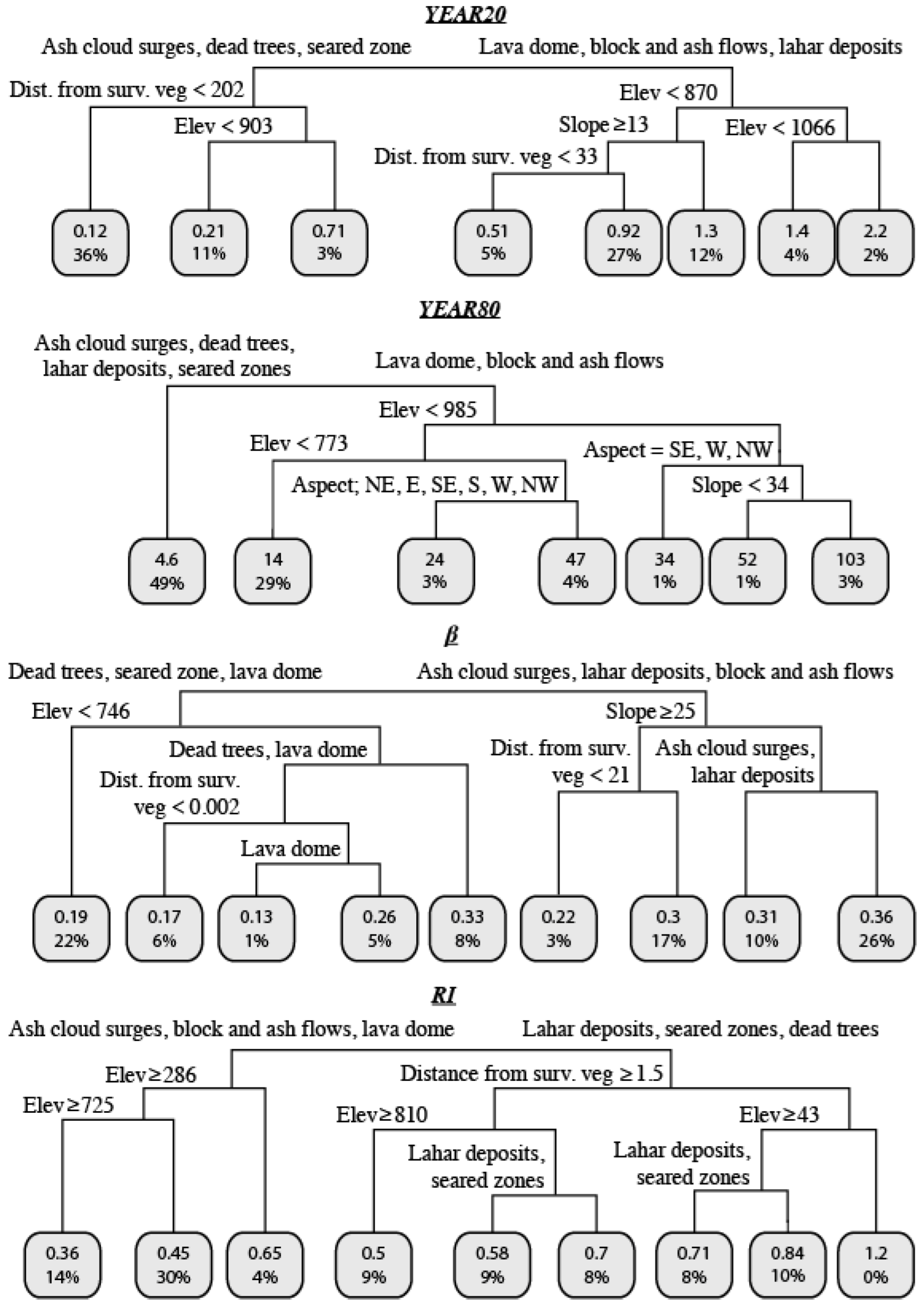
RTA results show that regression trees for each response variable explained about 57% to 47% of the variance in the datasets (Table 5). For all response variables, disturbance type was the variable used to apply the first split to the respective datasets (Table 5; Figure 8). For β, slope gradient and elevation governed the second split. For YEAR20 and RI, distance from surviving vegetation and elevation controlled the second split. For YEAR80, only elevation affected the second split (Table 5). Aspect and profile curvature featured rarely or not at all in the RTA results (Figure 8).

Table 5.
r2 values and top explanatory variables from the first two splits of the regression tree.
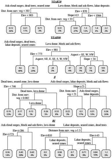
Figure 8.
Regression tree results for each recovery metric.
4. Discussion
Previous studies on post-eruption vegetation response have primarily used NDVI to measure vegetation response [19,23,24]. However, NDVI has been known to saturate quickly [39] and is less sensitive to vegetation damage severity compared to NBR [73]. While NBR was initially developed to measure ecological fire damage severity [35], in this study we proposed using NBR to quantify vegetation response in post-eruption landscapes due to the similarity in damage caused by volcanic eruptions and wildfires. Our results show that there are significant differences between NBR and NDVI responses during the earlier years of recovery, and for more intensely damaged areas. Compared to NDVI, NBR values in the short term show a more extensive range, suggesting a greater diversity of vegetation types or recovery states. Considering the spatial extent of the destruction area, greater diversity seems more ecologically plausible and is corroborated by the early (1996–2005) field study at Unzen volcano showing that average plant heights for herbaceous and woody vegetation showed different growth rates [46]. This result also aligns with other studies comparing NDVI and NBR responses to wildfire disturbances, which suggested that the larger NBR value range showed a greater capacity to distinguish different damage severity levels and vegetation structures [73], and that early NBR response was highly correlated to a field-based burn composite index [74]. Since NBR spectral bands are more sensitive to soil variation and background elements from burned areas [30], this agrees with the greater sensitivity of NBR during earlier stages of vegetation recovery where eruption damage products might be more similar to wildfire burned areas.
While the long-term NDVI and NBR responses show less significant differences across different disturbance zones, NBR indicated moderately longer times to reach 80% vegetation recovery (Figure 4B). This agrees with the previously established tendency of NDVI to saturate more quickly, especially under increasing vegetation cover [37,39,65], since aerial photos and our field observations also show that vegetation at the lava dome and block and ash areas is less recovered or homogenous than NDVI values indicate. Post-eruption vegetation at the lava dome and block and ash areas remains sparse, with only a light covering of grasses and small shrubs over some areas (Figure 9). However, at this spatial scale, mixed-pixel effects obscure our discussion on the extent to which the NBR response was affected by vegetation types, recovery states, or soil types [30]. Nevertheless, since the type of destruction and impact brought about by wildfires share many similarities with this type of volcanic eruption [75], using NBR may be an excellent choice to map and track early vegetation recovery in volcanic environments with heterogeneous damage severities and where pyroclastic flows had occurred.
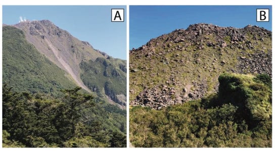
Figure 9.
Field photos taken by the lead author on 2 October 2021. (A): Eastern flank of the volcano. The background shows the eastern flank with the area affected by the block and ash flows and the lava dome still clearly demarcated. Only a light covering of grass and shrubs are present in that area. The foreground shows trees growing on the lower parts of the south-western slopes. (B): Southeast side of the summit (lava dome) area of the volcano. The background shows the summit area covered by a light smattering of grasses. In comparison, the foreground shows a more forested area (trees) on the lower southeast slopes of the volcano.
Our results for spatio-temporal vegetation responses show that the linear-log model used in previous studies [37,67] fit well, suggesting that a simple linear-log model can capture the recovery trend of post-eruption vegetation response over a longer-term period of almost 30 years and across different disturbance zones. This confirms the non-linear ecological responses to large disturbances, where early exponential growth may reflect the strong competitive advantage of early-arriving species or domineering topographic processes that can greatly influence vegetation trajectories [10]. Subsequent plateauing captures the reduced influence of initial dominant processes as ecosystem complexity grows and potentially stabilizes [7,20]. However, compared to previous studies, here our results show that the model fits better in more intensely disturbed zones, suggesting that it better characterizes responses from vegetation that was initially wholly destroyed (e.g., from block and ash flows). These areas, ecologically classified as primary succession sites, have little to no biological legacies due to the disturbance’s extreme intensity [76]. Comparatively, vegetation responses in areas not as severely damaged (ash cloud surges, dead trees, seared zones, lahar deposits) were not so well characterized by the linear-log model. There instead appears to be a sharper threshold dividing quicker and slower recovery rates that might be attributed to ecological dynamics and thresholds of existing vegetation interactions. The linear-log model also fits more poorly in areas with human intervention (i.e., dam building) or gullies. Dam building precludes vegetation growth, and gullies tend to be constantly reworked due to heavy rain, creating inconsistent vegetation regrowth that cannot be modelled well by a simple linear-log model. Since our study only used annual summer NBR composites, we left out seasonal variations that might be part of “boom-and-bust” ecological responses [76] that were not captured in this model. However, this is an avenue for future research. In addition, some recovery lengths for the lava dome area seemed excessively long ecologically; more than thousands of years. This may be because vegetation recovery at the lava dome is affected by volcanic smoke emissions which still persist and is too complex to be modelled by a simple linear-log model.
Finally, RTA results show that the chosen explanatory variables modelled all recovery metrics well and the primary disturbance type has most significant effect. This result aligns well with previous volcanic revegetation studies [16,20,22,23], where different disturbance types had stratified the landscape into zones of different vegetation recovery rates [23,40]. Additionally, in the short term, ecological factors such as distance from surviving vegetation have more significant effects due to the marked assistance for vegetation growth provided by surviving vegetation (Figure 8). In the long term, topographical and climate-related factors such as aspect and elevation play more prominent roles, as flora and fauna communities begin to stabilize and focus on growth rather than competition and survival [76]. Aerial seeding, which had occurred across most of Unzen volcano’s eruption area, is considered a secondary disturbance to vegetation recovery and succession trajectories [76]. While we did not include aerial seeding as an explanatory variable since it affected the majority of the study area and was assumed to be a spatially homogenous variable, the good model fitting results indicate that despite secondary disturbances, the primary (original) disturbance and topography still dominate vegetation recovery, although aerial seeding may have accelerated recovery rates across the board. Elevation as the second most influential response variable is likely due to correlations with the previously dropped explanatory variable: distance to crater, which represents the distance from the most intense eruption damage. For Unzen volcano, elevation is correlated to the damage intensity, since the eruption style comprised pyroclastic flows and ash cloud surges. Areas located further, i.e., at lower elevations, from the crater are more likely to experience less intense damage as eruption products weaken in intensity over longer distances.
Unexplained variance from the regression trees is likely due to stochastic elements that have occurred over time [22], as well as succession trajectory disruption due to aerial seeding efforts [21]. The Shimabara Peninsula also experiences heavy summer rainfall, and debris flows also occurred frequently during the rainy seasons after the eruption ended as unconsolidated material from the eruption was remobilized [44,77]. Consequently, some of the original surfaces of block and ash flow deposits were reworked and covered by lahar deposits [47], and erosion and debris flows may have interrupted expected recovery dynamics.
We also note that the RTA results and response metrics are limited by the 30 m resolution Landsat data, which likely obscured smaller-scale relationships. For example, microtopography affects seed survivability and growth by providing shade or protection from the elements [8]. However, this resolution cannot capture changes in small gullying or rilling processes that can create new microtopography [77]. In addition, we assumed that primary disturbance areas resulted in no surviving vegetation. However, such a sterile environment is rare in reality, and life has survived devastating disturbances by being buried or protected [16]. While this assumption might be acceptable at a 30 m resolution, future research using higher resolution remote sensing data should include more dynamic vegetation variables especially within primary disturbance zones to capture more comprehensive vegetation interactions.
5. Conclusions
In this study, we showed that historical Landsat images could be used to quantify short- and long-term vegetation responses to a large disturbance, and subsequently determined the factors of revegetation. We elucidated NBR and NDVI differences in tracking post-eruption vegetation response and proposed that at the 30 m pixel resolution, compared to the commonly used NDVI, NBR is a more precise indicator of vegetation regrowth especially during the early dynamic years of vegetation recovery because NBR better distinguishes vegetation’s damage severity and structural complexity. In characterizing the spatio-temporal vegetation response patterns, we showed that while vegetation recovery can be modelled using a simple linear-log function across different disturbance types, the linear-log function better models primary succession trajectories. Finally, using regression tree analyses, we showed that for the Unzen volcano study site, despite secondary disturbances, the primary disturbance type still has the most significant effect on post-eruption vegetation response in both the short and long term. While we focused on two popular indices to improve the transferability and scalability of results to other historical studies [19,23], one limitation of NBR and NDVI is their known sensitivity to vegetation types, soil moisture and variability, and lithology [30]. With increasing computing power and spectral resolutions, future research investigating narrower and different spectral band combinations can help to distinguish vegetation types or evaluate soil reflectance effects on vegetation indices [78,79]. Furthermore, while the dense Landsat time series provided enough data to run pixel-wise regressions, optical data are still hindered by clouds, thereby reducing the amount of analyzable data, which is disadvantageous during a time-sensitive process such as early vegetation recovery. Future vegetation recovery research fusing optical with other remote sensing types such as radar can help to overcome this issue. Incorporating data on erosion and soil production rates or a more nuanced treatment of disturbance types will also help validate drivers of vegetation recovery. Overall, the methodology and data presented here determined that landscape-scale post-disturbance vegetation responses can be more comprehensively quantified using easily-accessed Landsat images and vegetation indices, increasing applicability to other study sites, and contributing to a better understanding of ecology–geomorphology interactions.
Author Contributions
R.L. and T.O. conceptualized and designed the research. R.L. and C.Z. conducted data analyses. All authors have read and agreed to the published version of the manuscript.
Funding
This work was supported by JSPS KAKENHI Grant Number JP21H00627.
Data Availability Statement
Landsat data are openly available from the Google Earth Engine data catalog and can be referenced at the doi:10.1016/j.rse.2017.06.031. The 5-m digital elevation model is openly available from the Geospatial Information Authority of Japan’s Basic Map Information data catalog: “https://fgd.gsi.go.jp/download/menu.php (accessed on 1 May 2022)”. Generated secondary data and Python code used for processing data can be found with the GitHub repository doi:10.5281/zenodo.7239188.
Conflicts of Interest
The authors declare no conflict of interest. The funders had no role in the design of the study; in the collection, analyses, or interpretation of data; in the writing of the manuscript; or in the decision to publish the results.
References
- Istanbulluoglu, E. Vegetation-Modulated Landscape Evolution: Effects of Vegetation on Landscape Processes, Drainage Density, and Topography. J. Geophys. Res. 2005, 110, F02012. [Google Scholar] [CrossRef]
- Brantley, S.L.; Eissenstat, D.M.; Marshall, J.A.; Godsey, S.E.; Balogh-Brunstad, Z.; Karwan, D.L.; Papuga, S.A.; Roering, J.; Dawson, T.E.; Evaristo, J.; et al. Reviews and Syntheses: On the Roles Trees Play in Building and Plumbing the Critical Zone. Biogeosciences 2017, 14, 5115–5142. [Google Scholar] [CrossRef]
- Amundson, R.; Heimsath, A.; Owen, J.; Yoo, K.; Dietrich, W.E. Hillslope Soils and Vegetation. Geomorphology 2015, 234, 122–132. [Google Scholar] [CrossRef]
- Collins, D.B.G.; Bras, R.L. Climatic and Ecological Controls of Equilibrium Drainage Density, Relief, and Channel Concavity in Dry Lands. Water Resour. Res. 2010, 46. [Google Scholar] [CrossRef]
- Klaar, M.J.; Kidd, C.; Malone, E.; Bartlett, R.; Pinay, G.; Chapin, F.S.; Milner, A. Vegetation Succession in Deglaciated Landscapes: Implications for Sediment and Landscape Stability. Earth Surf. Process. Landf. 2015, 40, 1088–1100. [Google Scholar] [CrossRef]
- Schwarz, C.; Gourgue, O.; van Belzen, J.; Zhu, Z.; Bouma, T.J.; van de Koppel, J.; Ruessink, G.; Claude, N.; Temmerman, S. Self-Organization of a Biogeomorphic Landscape Controlled by Plant Life-History Traits. Nat. Geosci. 2018, 11, 672–677. [Google Scholar] [CrossRef]
- Marston, R.A. Geomorphology and Vegetation on Hillslopes: Interactions, Dependencies, and Feedback Loops. Geomorphology 2010, 116, 206–217. [Google Scholar] [CrossRef]
- Del Moral, R.; Grishin, S.Y. Volcanic Disturbances and Ecosystem Recovery. In Ecosystems of Disturbance Ground; Walker, L.R., Ed.; Elsevier Science: Amsterdam, The Netherlands, 1999; pp. 137–160. ISBN 978-0-08-055084-8. [Google Scholar]
- Pelletier, J.D.; Brad Murray, A.; Pierce, J.L.; Bierman, P.R.; Breshears, D.D.; Crosby, B.T.; Ellis, M.; Foufoula-Georgiou, E.; Heimsath, A.M.; Houser, C.; et al. Forecasting the Response of Earth’s Surface to Future Climatic and Land Use Changes: A Review of Methods and Research Needs. Earth’s Future 2015, 3, 220–251. [Google Scholar] [CrossRef]
- Viles, H.A.; Naylor, L.A.; Carter, N.E.A.; Chaput, D. Biogeomorphological Disturbance Regimes: Progress in Linking Ecological and Geomorphological Systems. Earth Surf. Process. Landf. 2008, 33, 1419–1435. [Google Scholar] [CrossRef]
- Rice, S.; Stoffel, M.; Turowski, J.M.; Wolf, A. Disturbance Regimes at the Interface of Geomorphology and Ecology. Earth Surf. Process. Landf. 2012, 37, 1678–1682. [Google Scholar] [CrossRef]
- Hales, T.C.; Ford, C.R.; Hwang, T.; Vose, J.M.; Band, L.E. Topographic and Ecologic Controls on Root Reinforcement. J. Geophys. Res. 2009, 114, F03013. [Google Scholar] [CrossRef]
- Hales, T.C. Modelling Biome-Scale Root Reinforcement and Slope Stability: Biome Driven Root Reinforcement Change. Earth Surf. Process. Landf. 2018, 43, 2157–2166. [Google Scholar] [CrossRef]
- Yunus, A.P.; Fan, X.; Tang, X.; Jie, D.; Xu, Q.; Huang, R. Decadal Vegetation Succession from MODIS Reveals the Spatio-Temporal Evolution of Post-Seismic Landsliding after the 2008 Wenchuan Earthquake. Remote Sens. Environ. 2020, 236, 111476. [Google Scholar] [CrossRef]
- Raab, T.; Krümmelbein, J.; Schneider, A.; Gerwin, W.; Maurer, T.; Naeth, M.A. Initial Ecosystem Processes as Key Factors of Landscape Development—A Review. Phys. Geogr. 2012, 33, 305–343. [Google Scholar] [CrossRef]
- Crisafulli, C.M.; Dale, V.H. (Eds.) Ecological Response to the 1980 Eruption of Mount St. Helens: Key Lessons and Remaining Questions. In Ecological Responses at Mount St. Helens: Revisited 35 Years after the 1980 Eruption; Springer: New York, NY, USA, 2018; pp. 1–18. ISBN 978-1-4939-7449-8. [Google Scholar]
- Dale, V.H.; Delgado-Acevedo, J.; MacMahon, J. Effects of Modern Volcanic Eruptions on Vegetation. In Volcanoes and the Environment; Marti, J., Ernst, G.G.J., Eds.; Cambridge University Press: Cambridge, UK, 2005; pp. 227–249. ISBN 978-0-521-59725-8. [Google Scholar]
- Tsuyuzaki, S. Vegetation Changes from 1984 to 2008 on Mount Usu, Northern Japan, after the 1977–1978 Eruptions. Ecol. Res. 2019, 34, 813–820. [Google Scholar] [CrossRef]
- De Rose, R.C.; Oguchi, T.; Morishima, W.; Collado, M. Land Cover Change on Mt. Pinatubo, the Philippines, Monitored Using ASTER VNIR. Int. J. Remote Sens. 2011, 32, 9279–9305. [Google Scholar] [CrossRef]
- Chinen, T.; Riviere, A. Post-Eruption Plant Recovery with Reference to Geomorphic Processes in the Summit Atrio of Mt. Usu, Japan. Geogr. Rev. Jpn. Ser. B 1989, 62, 35–55. [Google Scholar] [CrossRef][Green Version]
- Ogawa, Y.; Daimaru, H.; Chikashige, T. Hillside Restoration and Sediment Discharge after the 1990–1995 Eruption at Unzen Volcano, Japan. Water Sci. 2010, 54, 101–124. [Google Scholar] [CrossRef]
- Tsuyuzaki, S. Vegetation Recovery Patterns in Early Volcanic Succession. J. Plant Res. 1995, 108, 241–248. [Google Scholar] [CrossRef]
- Lawrence, R.L.; Ripple, W.J. Fifteen years of revegetation of Mount St. Helens: A landscape-scale analysis. Ecology 2000, 81, 2742–2752. [Google Scholar] [CrossRef]
- Teltscher, K.; Fassnacht, F.E. Using Multispectral Landsat and Sentinel-2 Satellite Data to Investigate Vegetation Change at Mount St. Helens since the Great Volcanic Eruption in 1980. J. Mt. Sci. 2018, 15, 1851–1867. [Google Scholar] [CrossRef]
- Solans Vila, J.P.; Barbosa, P. Post-Fire Vegetation Regrowth Detection in the Deiva Marina Region (Liguria-Italy) Using Landsat TM and ETM+ Data. Ecol. Model. 2010, 221, 75–84. [Google Scholar] [CrossRef]
- Baret, F.; Clevers, J.G.P.W.; Steven, M.D. The Robustness of Canopy Gap Fraction Estimates from Red and Near-Infrared Reflectances: A Comparison of Approaches. Remote Sens. Environ. 1995, 54, 141–151. [Google Scholar] [CrossRef]
- Veraverbeke, S.; Gitas, I.; Katagis, T.; Polychronaki, A.; Somers, B.; Goossens, R. Assessing Post-Fire Vegetation Recovery Using Red–near Infrared Vegetation Indices: Accounting for Background and Vegetation Variability. ISPRS J. Photogramm. Remote Sens. 2012, 68, 28–39. [Google Scholar] [CrossRef]
- Montandon, L.; Small, E. The Impact of Soil Reflectance on the Quantification of the Green Vegetation Fraction from NDVI. Remote Sens. Environ. 2008, 112, 1835–1845. [Google Scholar] [CrossRef]
- Ullah, S.; Si, Y.; Schlerf, M.; Skidmore, A.K.; Shafique, M.; Iqbal, I.A. Estimation of Grassland Biomass and Nitrogen Using MERIS Data. Int. J. Appl. Earth Obs. Geoinf. 2012, 19, 196–204. [Google Scholar] [CrossRef]
- Smith, A.M.S.; Eitel, J.U.H.; Hudak, A.T. Spectral Analysis of Charcoal on Soils: Implicationsfor Wildland Fire Severity Mapping Methods. Int. J. Wildland Fire 2010, 19, 976–983. [Google Scholar] [CrossRef]
- Decuyper, M.; Chávez, R.O.; Čufar, K.; Estay, S.A.; Clevers, J.G.P.W.; Prislan, P.; Gričar, J.; Črepinšek, Z.; Merela, M.; de Luis, M.; et al. Spatio-Temporal Assessment of Beech Growth in Relation to Climate Extremes in Slovenia—An Integrated Approach Using Remote Sensing and Tree-Ring Data. Agric. For. Meteorol. 2020, 287, 107925. [Google Scholar] [CrossRef]
- Wulder, M. Optical Remote-Sensing Techniques for the Assessment of Forest Inventory and Biophysical Parameters. Prog. Phys. Geogr. 1998, 22, 449–476. [Google Scholar] [CrossRef]
- Pickell, P.D.; Hermosilla, T.; Frazier, R.J.; Coops, N.C.; Wulder, M.A. Forest Recovery Trends Derived from Landsat Time Series for North American Boreal Forests. Int. J. Remote Sens. 2016, 37, 138–149. [Google Scholar] [CrossRef]
- Tucker, C.J. Red and Photographic Infrared Linear Combinations for Monitoring Vegetation. Remote Sens. Environ. 1979, 8, 127–150. [Google Scholar] [CrossRef]
- Key, C.H.; Benson, N.C. Landscape Assessment: Ground Measure of Severity, the Composite Burn Index; and Remote Sensing of Severity, the Normalized Burn Ratio; FIREMON: Fire Effects Monitoring and Inventory System; USDA Forest Service, Rocky Mountain Research Station: Ogden, UT, USA, 2006; pp. LA1–LA51. [Google Scholar]
- Purevdorj, T.S.; Tateishi, R.; Ishiyama, T.; Honda, Y. Relationships between Percent Vegetation Cover and Vegetation Indices. Int. J. Remote Sens. 1998, 19, 3519–3535. [Google Scholar] [CrossRef]
- Díaz-Delgado, R.; Salvador, R.; Pons, X. Monitoring of Plant Community Regeneration after Fire by Remote Sensing. In Fire Management and Landscape Ecology; International Association of Wildland Fire: Missoula, MT, USA, 1998; pp. 315–324. [Google Scholar]
- Prabhakara, K.; Hively, W.D.; McCarty, G.W. Evaluating the Relationship between Biomass, Percent Groundcover and Remote Sensing Indices across Six Winter Cover Crop Fields in Maryland, United States. Int. J. Appl. Earth Obs. Geoinf. 2015, 39, 88–102. [Google Scholar] [CrossRef]
- Carlson, T.N.; Ripley, D.A. On the Relation between NDVI, Fractional Vegetation Cover, and Leaf Area Index. Remote Sens. Environ. 1997, 62, 241–252. [Google Scholar] [CrossRef]
- White, J.C.; Wulder, M.A.; Hermosilla, T.; Coops, N.C.; Hobart, G.W. A Nationwide Annual Characterization of 25 Years of Forest Disturbance and Recovery for Canada Using Landsat Time Series. Remote Sens. Environ. 2017, 194, 303–321. [Google Scholar] [CrossRef]
- Frazier, R.J.; Coops, N.C.; Wulder, M.A.; Hermosilla, T.; White, J.C. Analyzing Spatial and Temporal Variability in Short-Term Rates of Post-Fire Vegetation Return from Landsat Time Series. Remote Sens. Environ. 2018, 205, 32–45. [Google Scholar] [CrossRef]
- Kottek, M.; Grieser, J.; Beck, C.; Rudolf, B.; Rubel, F. World Map of the Köppen-Geiger Climate Classification Updated. Meteorol. Z. 2006, 15, 259–263. [Google Scholar] [CrossRef]
- Kawamoto, K.; Maeda, H.; Soeyama, H. The State of Vegetation around Runout Zone of Pyroclastic Flow at Mt. Fugen in Unzen. Kyushu J. For. Res. 2010, 63, 185–186. [Google Scholar]
- Nakada, S.; Shimizu, H.; Ohta, K. Overview of the 1990–1995 Eruption at Unzen Volcano. J. Volcanol. Geotherm. Res. 1999, 89, 1–22. [Google Scholar] [CrossRef]
- Hoshizumi, H.; Uto, K.; Watanabe, K. Geology and Eruptive History of Unzen Volcano, Shimabara Peninsula, Kyushu, SW Japan. J. Volcanol. Geotherm. Res. 1999, 89, 81–94. [Google Scholar] [CrossRef]
- Biodiversity Center of Japan 1/50,000 Vegetation Map “Shimabara” GIS Data. 1985. Available online: http://www.biodic.go.jp/reports2/3rd/vgt_42/index.html (accessed on 13 January 2021).
- Miyabuchi, Y. Deposits Associated with the 1990–1995 Eruption of Unzen Volcano, Japan. J. Volcanol. Geotherm. Res. 1999, 89, 139–158. [Google Scholar] [CrossRef]
- Sakai, M.; Kobayashi, M.; Imaya, A.; Kuroiwa, Y.; Kotou, H.; Sato, T.; Saito, S.; Nagamatsu, D.; Kominami, Y.; Inagaki, M.; et al. A study of a volcanic succession process at Taruki of Unzen. Kyushu J. For. Res. 2006, 59, 249–251. [Google Scholar]
- Ogawa, Y.; Akema, T.; Daimaru, H. A field survey of revegetation plants and field observation of overland flow on slopes overlain by pyroclastic-flow de-posits, Unzen volcano, Japan. J. Jpn. Soc. Eros. Control Eng. 2011, 63, 78–82. [Google Scholar] [CrossRef]
- Ogawa, Y.; Akema, T.; Daimaru, H. The Growth of Woody Plant in the Past Four Years on a Slope Revegetated by Aerial Seeding Works of Mount Fugen. Kyushu J. For. Res. 2005, 58, 218–220. [Google Scholar]
- Ogawa, Y.; Daimaru, H.; Shimizu, A. Experimental Study of Post-Eruption Overland Flow and Sediment Load from Slopes Overlain by Pyroclastic-Flow Deposits, Unzen Volcano, Japan. Geomorphol. Relief Process. Environ. 2007, 13, 237–246. [Google Scholar] [CrossRef]
- Yamauchi, T.; Ideguchi, K. Unzen Fugendake greenery restoring forest conservation project. J-STAGE 2016, 60, 129–142. [Google Scholar] [CrossRef]
- Inoue, G.; Nagaoka, K.; Sugiyama, S. Buried humus soil at the northern and southern foot of Unzen volcano. J-STAGE 2010, 56, 98. [Google Scholar] [CrossRef]
- Gorelick, N.; Hancher, M.; Dixon, M.; Ilyushchenko, S.; Thau, D.; Moore, R. Google Earth Engine: Planetary-Scale Geospatial Analysis for Everyone. Remote Sens. Environ. 2017, 202, 18–27. [Google Scholar] [CrossRef]
- Masek, J.G.; Vermote, E.F.; Saleous, N.E.; Wolfe, R.; Hall, F.G.; Huemmrich, K.F.; Gao, F.; Kutler, J.; Lim, T.-K. A Landsat Surface Reflectance Dataset for North America, 1990–2000. IEEE Geosci. Remote Sens. Lett. 2006, 3, 68–72. [Google Scholar] [CrossRef]
- EROS Data Center U.S. Geological Survey. Preliminary Assessment of the Value of the Landsat ETM+ Data Following Scan Line Corrector Malfunction. 2003. Available online: https://d9-wret.s3.us-west-2.amazonaws.com/assets/palladium/production/s3fs-public/atoms/files/SLC_off_Scientific_Usability.pdf (accessed on 15 January 2022).
- EROS Data Center U.S. Geological Survey. USGS/EROS LSDS-1414, Version 3, Landsat 7 (L7) Enhanced Thematic Mapper Plus (ETM+) Section 2 (S2) Level 1 (L1) Data Format Control Book (DFCB). 2020. Available online: https://d9-wret.s3.us-west-2.amazonaws.com/assets/palladium/production/s3fs-public/atoms/files/LSDS-1414_Landsat7ETM-C2-L1-DFCB-v3.pdf (accessed on 15 January 2022).
- Zhu, Z.; Wang, S.; Woodcock, C.E. Improvement and Expansion of the Fmask Algorithm: Cloud, Cloud Shadow, and Snow Detection for Landsats 4–7, 8, and Sentinel 2 Images. Remote Sens. Environ. 2015, 159, 269–277. [Google Scholar] [CrossRef]
- Roy, D.P.; Kovalskyy, V.; Zhang, H.K.; Vermote, E.F.; Yan, L.; Kumar, S.S.; Egorov, A. Characterization of Landsat-7 to Landsat-8 Reflective Wavelength and Normalized Difference Vegetation Index Continuity. Remote Sens. Environ. 2016, 185, 57–70. [Google Scholar] [CrossRef] [PubMed]
- Hurni, K.; Van Den Hoek, J.; Fox, J. Assessing the Spatial, Spectral, and Temporal Consistency of Topographically Corrected Landsat Time Series Composites across the Mountainous Forests of Nepal. Remote Sens. Environ. 2019, 231, 111225. [Google Scholar] [CrossRef]
- Pelletier, J.D.; Barron-Gafford, G.A.; Gutiérrez-Jurado, H.; Hinckley, E.S.; Istanbulluoglu, E.; McGuire, L.A.; Niu, G.; Poulos, M.J.; Rasmussen, C.; Richardson, P.; et al. Which Way Do You Lean? Using Slope Aspect Variations to Understand Critical Zone Processes and Feedbacks. Earth Surf. Process. Landf. 2018, 43, 1133–1154. [Google Scholar] [CrossRef]
- Griffiths, R.P.; Madritch, M.D.; Swanson, A.K. The Effects of Topography on Forest Soil Characteristics in the Oregon Cascade Mountains (USA): Implications for the Effects of Climate Change on Soil Properties. For. Ecol. Manag. 2009, 257, 1–7. [Google Scholar] [CrossRef]
- Baartman, J.E.M.; Temme, A.J.A.M.; Saco, P.M. The Effect of Landform Variation on Vegetation Patterning and Related Sediment Dynamics. Earth Surf. Process. Landf. 2018, 43, 2121–2135. [Google Scholar] [CrossRef]
- Biodiversity Center of Japan 1/50,000 Vegetation Map “Shimabara” GIS Data. 1994. Available online: https://www.biodic.go.jp/kiso/vg/vg_kiso.html#mainText (accessed on 13 January 2021).
- Hislop, S.; Jones, S.; Soto-Berelov, M.; Skidmore, A.; Haywood, A.; Nguyen, T. Using Landsat Spectral Indices in Time-Series to Assess Wildfire Disturbance and Recovery. Remote Sens. 2018, 10, 460. [Google Scholar] [CrossRef]
- Sullivan, G.M.; Feinn, R. Using Effect Size—Or Why the P Value Is Not Enough. J. Grad. Med. Educ. 2012, 4, 279–282. [Google Scholar] [CrossRef]
- De Schutter, A.; Kervyn, M.; Canters, F.; Bosshard-Stadlin, S.A.; Songo, M.A.M.; Mattsson, H.B. Ash Fall Impact on Vegetation: A Remote Sensing Approach of the Oldoinyo Lengai 2007–08 Eruption. J. Appl. Volcanol. 2015, 4, 15. [Google Scholar] [CrossRef]
- Senf, C.; Müller, J.; Seidl, R. Post-Disturbance Recovery of Forest Cover and Tree Height Differ with Management in Central Europe. Landsc. Ecol. 2019, 34, 2837–2850. [Google Scholar] [CrossRef]
- Kennedy, R.E.; Yang, Z.; Cohen, W.B.; Pfaff, E.; Braaten, J.; Nelson, P. Spatial and Temporal Patterns of Forest Disturbance and Regrowth within the Area of the Northwest Forest Plan. Remote Sens. Environ. 2012, 122, 117–133. [Google Scholar] [CrossRef]
- Breiman, L.; Friedman, J.H.; Olshen, R.A.; Stone, C.J. Classification and Regression Trees, 1st ed.; Routledge: London, UK, 2017; ISBN 978-1-315-13947-0. [Google Scholar]
- Saito, H.; Uchiyama, S.; Teshirogi, K. Rapid Vegetation Recovery at Landslide Scars Detected by Multitemporal High-Resolution Satellite Imagery at Aso Volcano, Japan. Geomorphology 2022, 398, 107989. [Google Scholar] [CrossRef]
- Therneau, T.; Atkinson, B.; Ripley, B. Rpart: Recursive Partitioning. R Package Version 4.1-16. 2022. Available online: http://CRAN.R-project.org/package=rpart (accessed on 1 May 2022).
- Escuin, S.; Navarro, R.; Fernández, P. Fire Severity Assessment by Using NBR (Normalized Burn Ratio) and NDVI (Normalized Difference Vegetation Index) Derived from LANDSAT TM/ETM Images. Int. J. Remote Sens. 2008, 29, 1053–1073. [Google Scholar] [CrossRef]
- Epting, J.; Verbyla, D. Landscape-Level Interactions of Prefire Vegetation, Burn Severity, and Postfire Vegetation over a 16-Year Period in Interior Alaska. Can. J. For. Res. 2005, 35, 1367–1377. [Google Scholar] [CrossRef]
- Chuvieco, E.; Mouillot, F.; van der Werf, G.R.; San Miguel, J.; Tanase, M.; Koutsias, N.; García, M.; Yebra, M.; Padilla, M.; Gitas, I.; et al. Historical Background and Current Developments for Mapping Burned Area from Satellite Earth Observation. Remote Sens. Environ. 2019, 225, 45–64. [Google Scholar] [CrossRef]
- Crisafulli, C.M.; Swanson, F.J.; Halvorson, J.J.; Clarkson, B.D. Volcano Ecology: Disturbance Characteristics and Assembly of Biological Communities. In The Encyclopedia of Volcanoes; Elsevier: Amsterdam, The Netherlands, 2015; pp. 1265–1284. ISBN 978-0-12-385938-9. [Google Scholar]
- Tsunetaka, H.; Shinohara, Y.; Hotta, N.; Gomez, C.; Sakai, Y. Multi-decadal Changes in the Relationships between Rainfall Characteristics and Debris-flow Occurrences in Response to Gully Evolution after the 1990–1995 Mount Unzen Eruptions. Earth Surf. Process. Landf. 2021, 46, 2141–2162. [Google Scholar] [CrossRef]
- Fei, Y.; Jiulin, S.; Hongliang, F.; Zuofang, Y.; Jiahua, Z.; Yunqiang, Z.; Kaishan, S.; Zongming, W.; Maogui, H. Comparison of Different Methods for Corn LAI Estimation over Northeastern China. Int. J. Appl. Earth Obs. Geoinf. 2012, 18, 462–471. [Google Scholar] [CrossRef]
- Ren, H.; Zhou, G. Estimating Green Biomass Ratio with Remote Sensing in Arid Grasslands. Ecol. Indic. 2019, 98, 568–574. [Google Scholar] [CrossRef]
Publisher’s Note: MDPI stays neutral with regard to jurisdictional claims in published maps and institutional affiliations. |
© 2022 by the authors. Licensee MDPI, Basel, Switzerland. This article is an open access article distributed under the terms and conditions of the Creative Commons Attribution (CC BY) license (https://creativecommons.org/licenses/by/4.0/).

