Article

Spatial-Temporal Relationship Analysis of Vegetation Phenology and Meteorological Parameters in an Agro-Pasture Ecotone in China

1
College of Civil Engineering, Nanjing Forestry University, Nanjing 210037, China
2
Key Laboratory of Digital Earth Science, Institute of Remote Sensing and Digital Earth (RADI), Chinese Academy of Sciences (CAS), Beijing 100094, China
3
International Centre on Space Technologies for Natural and Cultural Heritage under the Auspices of UNESCO, Beijing 100094, China
*
Author to whom correspondence should be addressed.
Remote Sens. 2022, 14(21), 5417; https://doi.org/10.3390/rs14215417
Submission received: 29 June 2022 / Revised: 26 October 2022 / Accepted: 27 October 2022 / Published: 28 October 2022

Abstract

:
Vegetation phenology is a sensitive indicator of climate change, and can help understand the response of vegetation cycles to climate, which is important for understanding the impact of global climate change on terrestrial ecosystems. In this study, based on the enhanced vegetation index (EVI) time-series data, derived from the moderate-resolution imaging spectroradiometer (MODIS) data, the climate parameters were extracted using the Savitzky–Golay (S–G) filtering method to explore the spatial and temporal variation characteristics of the vegetation phenology in an agro-pasture ecotone in China, from 2000 to 2020. In addition, the response characteristics of the vegetation phenology to the climate elements (temperature and precipitation) were also analyzed. The results showed the following: (1) The start of the growing season (SOS) was widely advanced, and that was caused by climate change. The end of the growing season (EOS) was delayed, and the length of the growing season (LOS) was gradually extended with a large interannual fluctuation in the SOS and the LOS in the region; (2) the SOS showed significant negative correlations with the air temperature and precipitation. Precipitation was mainly positively correlated with the EOS, but there was no significant difference in the correlation between temperature and the EOS. In general, pre-season precipitation is the main driver of the vegetation phenology, while the influence of temperature on the phenology is less obvious; (3) in the semi-arid area and arid area, the phenology was mainly influenced by precipitation. The response of the vegetation phenology to the temperatures in different temperature zones was found to be regular, showing high spatial differences. In general, the higher the cumulus temperature, the lower the negative effect of the temperature on both the SOS and EOS. These results may provide new reference to study the non-systematic changes of the vegetation phenology in response to climate change.

1. Introduction

Vegetation phenology is mainly the study of repeated seasonal phenomena of vegetation that occur in an annual cycle under the influence of the natural environment or human factors, such as plant germination, leaf spreading, flowering, fruiting, leaf discoloration, and defoliation [1,2,3]. The high sensitivity of vegetation to changes in the external environment can be indicated by changes in these phenological indicators [4,5]. In addition, climate change is the most important factor of environmental change [6]. Therefore, studying the relationship between these phenological indicators and meteorological parameters (e.g., precipitation and temperature) is important for a better understanding of the response relationship between climate change and vegetation phenology trends [7,8].
The current vegetation phenology research methods mainly include the traditional ground-based monitoring methods and remote sensing monitoring methods [9]. Traditional phenology observation mainly uses visual observation methods, based on field observations, i.e., direct fixed-point observations of intra-annual and inter-annual variations in vegetation phenology [10,11]. In early phenological observations, researchers have found that the interannual change of the climate will cause the dynamic change of the vegetation phenology by using phenological observation data and climate data [1,12]. Rosenzweig et al. [13] studied the effects of climate change on the phenology, based on 542 vegetation phenological observations, from 1971 to 2000. The results showed that 78% of the vegetation samples had a tendency to advance leaf spread, flowering, and fruiting, but leaf discoloration and defoliation had a tendency to be delayed. Meng et al. [14] observed six deciduous tree species in the Pan-European Phenology Project, from 1980 to 2016, and found that the regulation by photoperiod would slow down the advance of the spring vegetation phenology in the context of climate warming. Walther et al. [1] found that climate warming has a significant impact on the vegetation phenology in the recent 30 years, which reflects the response and adaptation of the vegetation to climate change. Therefore, long-term ground-based phenological observation networks are particularly useful in investigating the phenological changes and responses to climate change. However, this method is limited to the species that can be observed, to the coverage area, to discontinuous time spans, and to the effort required, therefore it is seldom applied to large-scale phenology studies [15]. With the development of remote sensing technology from the 1970s, many scholars have applied vegetation indices, such as NDVI and EVI, to study the vegetation phenology in different regions at different time periods, which has contributed to the later macroscopic phenology studies in the context of global climate change [16,17]. Nowadays, this method is widely used in the fields of agricultural production, socio-economic activities, ecological research, and global change [18].
Since global climate change caused by warming, has been proposed, researchers have been increasingly concerned about the effects of climate change on vegetation [19,20]. Of all of the phenology parameters, the start of the growing season (SOS) and the end of the growing season (EOS) are most sensitive to climate change, which is manifested by the delay or advancement of the SOS and EOS [21]. Most studies have demonstrated that the SOS is triggered by pre-season temperatures [22]. For example, Piao et al. [23] used NDVI data to explore the response of the spring phenology on the Tibetan Plateau under climate change, from 1982 to 2006, and showed that the SOS was correspondingly advanced by 4.1 d while the temperature increased by 1 °C. Therefore, warmer temperatures, due to global warming, will lead to an overall earlier SOS and a delayed EOS, resulting in a corresponding increase in the length of the growing season (LOS) [24,25]. Moreover, it has been reported that the interaction between the maximum and minimum temperatures is the most important determinant of the vegetation phenology changes [26]. Over the past 30 years, the trend of increasing temperatures has been more remarkable in middle-high latitude regions, such as Eurasia, and several surveys have found that the spring phenology has started to advance in the Northern Hemisphere [27,28]. Although it is generally accepted that temperature is the main cause of the vegetation phenology changes, the regulation of the phenology by temperature alone can hardly explain the changes under environmental changes [29]. Recent research has found that changes in precipitation, due to climate warming, can also cause changes in the vegetation phenology, the magnitude of which varies by location, species, and study period [30,31]. In arid and semi-arid zones or other areas with a relatively low precipitation, such as the Gobi Desert and the grasslands, precipitation has a greater effect on phenology than temperature [22,32]. In these regions, the growth of plants showed a strong positive correlation with precipitation [33]. Correspondingly, in areas with a high precipitation, the growth of vegetation showed a lower or negative correlation with precipitation [33,34]. For example, Wu et al. found that the SOS was delayed while the EOS was advanced, in the arid regions of Central Asia [33]. However, at high latitudes and high altitudes, the effect of a reduced precipitation on the phenology was not significant, due to their high soil moisture availability [35]. Instead, its vegetation phenology is mainly limited by the temperature [35]. However, a decrease in precipitation and an increase in temperature were not found to have a significant effect on the phenology. Therefore, the sensitivity to precipitation and temperature varies from region to region, even in the same location, the different time periods may show differences in the sensitivity of the vegetation phenology to precipitation and temperature.
The agro-pasture ecotone in China that we studied, includes six temperature zones and four dry and wet zones (Table 1), with large natural geographic gradients, diverse vegetation evolutionary processes, and is extremely sensitive ecosystem responses to climate change [36]. Additionally, the agro-pasture ecotone is an ecological transition zone connecting agriculture and animal husbandry, also known as the semi-agricultural and semi-pastoral zone [37,38]. As a production interface of two food systems in China, the agro-pasture ecotone has the potential for serious soil erosion and land desertification, so it is also an ecologically fragile zone in China [39]. However, previous studies on the agro-pasture ecotone mainly focused on land use change and climate change, ignoring the fragility of the ecosystem in the agro-pasture ecotone itself. Vegetation is an important part of the ecosystem, and the vegetation phenology is an important indicator of the vegetation growth. Although studies have been conducted on the phenology of some parts of the agro-pasture ecotone, the influence of the climatic parameters on the vegetation phenology has not been analyzed [40]. Therefore, we studied the vegetation phenology in the agro-pasture ecotone to better understand the current trends in the context of climate change. Based on the 16-day synthetic MODIS EVI dataset, we used the Savitzky–Golay (S–G) filter to reconstruct the EVI time series data, and used the maximum slope method to extract the key parameters of the vegetation phenology (i.e., SOS, EOS and LOS) in the agro-pasture ecotone, from 2000 to 2020. The main objectives of this study were to: (1) study the spatial and temporal variability of the vegetation phenology in the different eco-geographic regions of the agro-pasture ecotone, from 2000 to 2020; (2) assess the influence of the monthly temperature and precipitation on the vegetation phenology in the study area; (3) explore the response mechanisms between the vegetation phenology and the climate factors in the study area. This study will provide a scientific basis for agricultural and livestock production, the reasonable rotation of grazing land, and ecological environment construction in the region.

2. Data and Methods

2.1. Study Area

The agro-pasture ecotone (Figure 1a,b) is distributed from northeast to southwest across China (95°~125°E, 25°~48°N), with a total area of about 1.03 million km2, accounting for about 1/9 of China’s total land area [37,39]. From a general point of view, it can be divided into the southern agro-pasture ecotone and the northern agro-pasture ecotone. The southern agro-pasture ecotone belongs to a humid and semi-humid area, with an annual precipitation of 600~800 mm and better climatic conditions, and is a transition zone between the Tibetan Plateau and the Sichuan Basin for agriculture and animal husbandry, with its vegetation mainly located in woodland, scrubland, and meadows (Figure 1a). Its topography is mainly high mountains and plateau landscapes, with an overall high and undulating terrain (Figure 1b) [41]. The northern agro-pasture ecotone is an arid and semi-arid region with an annual precipitation of 250~500 mm and relatively harsh climatic conditions. The region has widespread plateaus, mountains, and deserts, and grassland is its main vegetation type [42]. The agro-pasture ecotone is the intersection and transition area between the agricultural cultivation area and the grassland animal husbandry area in China. The zone is not only semi-agricultural and semi-pastoral, but also agricultural and pastoral at times, which is the largest ecological transition area and an ecologically fragile area in China. As people did not use scientific farming and animal husbandry methods in this area in the past, the outlook of the ecological environment of the agro-pasture ecotone is not optimistic [38]. At present, scholars in China have mainly studied land use, landscape patterns, the ecological environment, and desertification in the agro-pasture ecotone, but there have been few reports on the spatial and temporal patterns of the vegetation in the agro-pasture ecotone over a long period of time. Therefore, it is important to study the vegetation patterns in the whole agro-pasture ecotone.

2.2. Data Sources and Preprocessing

2.2.1. MODIS EVI

The EVI time series data used in this study were obtained from the MOD13Q1 vegetation index dataset, from 2000 to 2020, provided by the NASA data website (https://modis.gsfc.nasa.gov (accessed on 30 September 2021)), with a temporal resolution of 16 d and a spatial resolution of 250 m × 250 m, and a total of 480 image periods [43,44]. This dataset is the standard terrestrial thematic MODIS Level 3 product containing NDVI, the enhanced vegetation index (EVI), and other reflectance products, where the effective values of the vegetation index range from −2000 to 10,000.
The jagged EVI time-series curves obtained, are inevitably interspersed with various noises and interferences, due to the sensors themselves, as well as random disturbances, such as clouds, atmospheric aerosols, surface water, snow, and ice. It is therefore necessary to reconstruct the EVI time series curves [45,46]. In this paper, the EVI time series was reconstructed using Savitzky–Golay (S–G) filtering [47], which is a least-squares convolution fitting method and a polynomial fitting method, based on the local features of the curve. The model is calculated as follows [47]:
y j * = i = m i = m C i × Y j + i N
where Yj+i is the value of the original EVI time series data; Y j * is the fitted value of the EVI time series data; Ci is the correlation coefficient of the i-th EVI value of this sliding window; N is the number of convolutions; and m is the sliding window size.
In addition, we also exclude the image elements with an annual mean EVI of less than 0.1, from 2000 to 2020, which were not involved in the phenology calculations, in order to further reduce the uncertainty of the bare soil, desert, water bodies, and sparse vegetation on the EVI trend study [48].

2.2.2. Meteorological Data

Because of the small number of meteorological stations, it was difficult to achieve the accuracy required for this study. Therefore, the meteorological data (monthly average temperature and precipitation) from the National Earth System Science Data Center, National Science & Technology Infrastructure of China (http://www.geodata.cn (accessed on 12 April 2022)) were used, which has a temporal resolution of months and a spatial resolution of 0.0083333° (about 1 km) [49]. The dataset we selected is the month-by-month data from 2000 to 2020. The data set is based on the global 0.5° climate dataset published by the Climactic Research Unit (CRU) and the global high-resolution climate dataset published by WorldClim, and is downscaled for use in China by the Delta spatial downscaling scheme and validated by 496 ground-based meteorological stations [49,50].
In order to achieve the same spatial resolution as that of the EVI data, we applied the inverse distance weighting method to the meteorological data, which facilitated the subsequent analysis and required the dimensionless processing of the meteorological data.

2.2.3. Eco-Geographical Data

The eco-geographical regional systems mainly reflect the geographical differences in natural elements, such as the temperature and wet and dry conditions, and can be used as a macro framework for monitoring ecological and environmental characteristics [51]. The study of the vegetation phenological changes from the perspective of eco-geographic regions can better reveal the characteristics of the regional phenological differences in the agro-pasture ecotone. In this study, the framework of China’s eco-geographical regional system, developed by Zheng et al. was used to divide the agro-pasture ecotone into 10 natural areas (Table 1 and Figure 1) [51].

2.2.4. Other Data

The GlobeLand30 dataset contains 30 m resolution global land cover data, provided by the National Basic Geographic Information Center (http://www.globallandcover.com (accessed on 5 March 2022)). The dataset contains 10 types of land cover data, namely, cultivated land, forest, grassland, shrublands, bodies of water, wetlands, tundra, artificial surfaces, bare ground, glaciers and permanent snow [52,53]. To reduce the impact of the anthropogenic changes on the vegetation over 21 years, we only selected land cover types (grassland, forest, and shrubland) that remained unchanged between 2000, 2010, and 2020. The DEM data comes from the ASTER GDEM V2 dataset, downloaded from Geospatial Data Cloud (http://www.gscloud.cn (accessed on 5 March 2022)). The DEM data were stitched and masked in ArcMap and resampled to 250 m.

2.3. Data Analysis Methods

2.3.1. Extraction of the Data on the Vegetation Phenology

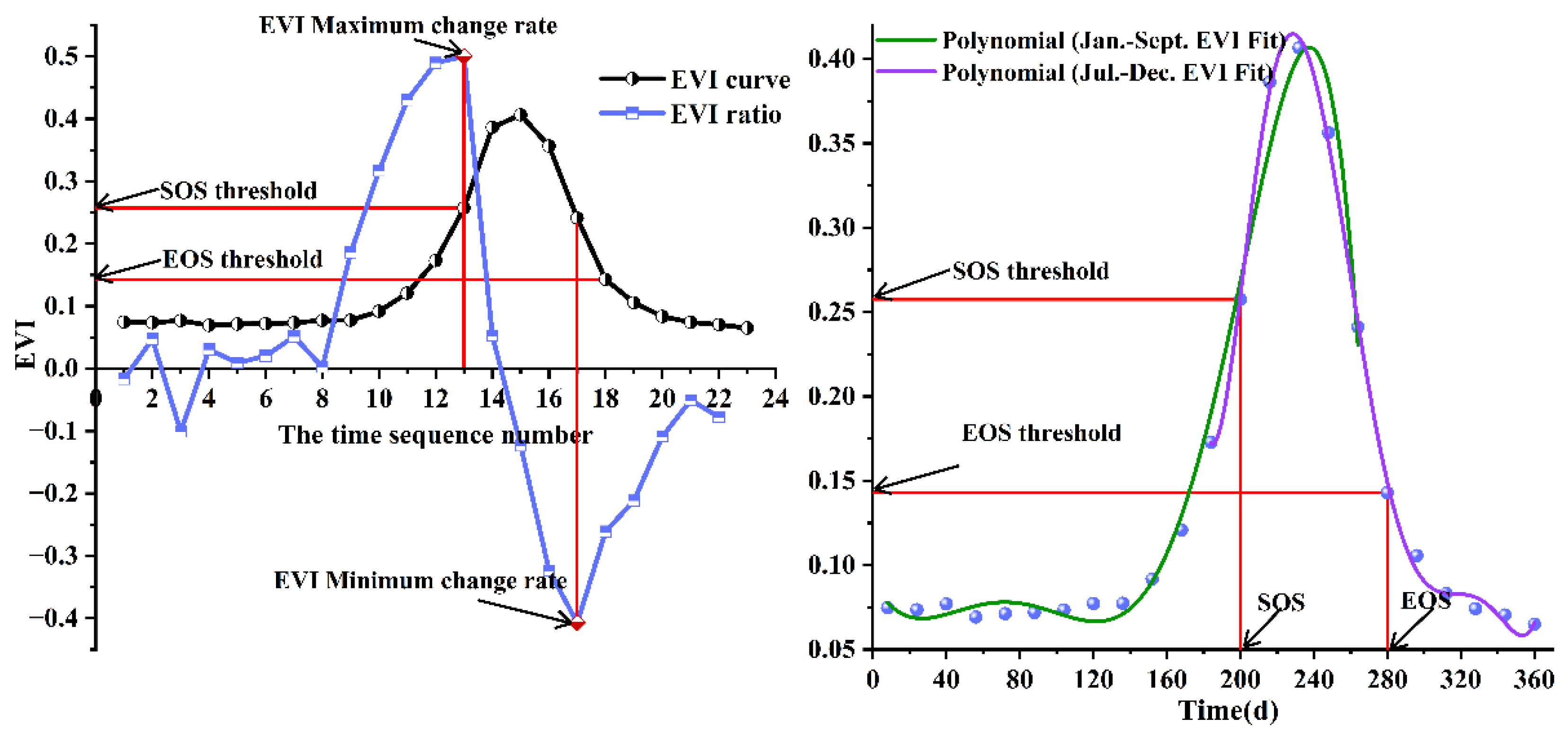
In this study, the vegetation phenology was extracted using the Polyfit-Maximum [48], which uses the maximum rate of change of the EVI and the minimum rate of change of the EVI to extract the SOS and EOS, respectively, and has been proved to be applicable to the extraction of the vegetation phenology parameters at large scales and has therefore been widely used in previous studies [54,55,56]:
EVI ration ( t ) = EVI ( t + 1 ) EVI ( t ) EVI ( t )
where t is time (time resolution 16 d); EVI(t) is the EVI value at time t; and EVIration(t) is the rate of change of the EVI at time t. The moment t corresponding to the maximum EVIration(t) was found, and the EVI(t) at moment t was used as the threshold for the SOS; the moment t corresponding to the minimum EVIration(t) was found, and the EVI(t + 1) at moment t + 1 was used as the threshold for extracting the EOS. Then, the EVI time-series data points from January to September (SOS) and June to December (EOS) of each year were fitted separately, using the polynomial fitting method to reconstruct them as 1 d EVI time series with a temporal resolution [28,48]:
EVI = a 0 + a 1 x + a 2 x 2 + + a n x n
where x is the day (Julian day) related to the EVI time series in each year; n is the number of polynomials, which, after validation and comparison, was found to be better at fitting the vegetation curves throughout the growing season when n = 6; and a0, a1, a2, …, an are the coefficients of the regression fit (Figure 2). Finally, the SOS and EOS were extracted from the reconstructed daily EVI time-series curves, using the SOS and EOS thresholds obtained earlier for each time series image element. The LOS is the difference between the EOS and SOS.

2.3.2. Trend Analysis Based on Theil–Sen’s Slope and the Mann–Kendall Test

Although least squares-based linear trend regression models are widely used in time-series analyses, they are susceptible to outliers in the time-series [57,58]. The Theil–Sen median trend analysis [57] is often used to detect trends in long time-series data-sets, as it not only avoids the effect of missing data and data distribution patterns in the time-series for the analysis results, but also removes the effect of outliers in the time-series for the analysis results. The model is calculated as follows [57]:
β = m e d i a n ( x j x i j i )       1 < i < j < n
where the trend degree β value represents the trend of the series; xj and xi represent the series values at moments j and i, respectively; it indicates an upward trend when β > 0, a downward trend when β < 0, an insignificant trend when β = 0.
The Mann–Kendall method for the trend analysis [59,60] is a non-parametric statistical test, which has the advantage of not requiring the sample to obey a certain distribution, it is suitable for non-normally distributed data, and is not disturbed by a few outliers; it is also often used to detect the significance of the time-series trends [59,60].
S = i = 1 n 1 j = i + 1 n sgn ( x j x i )
sgn ( x j x i ) = { 1 ( x j x i > 0 ) 0 ( x j x i = 0 ) 1 ( x j x i < 0 )
V a r ( S ) = n ( n 1 ) ( 2 n + 5 ) 18
Z = { S 1 V a r ( S ) ( S > 0 ) 0 ( S = 0 ) S + 1 V a r ( S ) ( S < 0 )
where xi and xj are the i-th and j-th data values of the time series, respectively; n is the length of the time-series; and sgn is the sign function. Z follows a standard normal distribution. Z is the trend of the time-series data; and means an increasing trend over time when Z > 0, and a decreasing trend when Z < 0.
The Mann–Kendall method uses a bilateral trend test, which is based on the null hypothesis H0: β = 0. The null hypothesis is rejected when |Z| > Z1−α/2, i.e., the trend is significant; the opposite indicates that the trend is not significant, where Z1−α/2 is the standard normal distribution and α is the significance test level. In this paper, α is set as 0.05, and Z1−α/2 is set as ±1.96. When the absolute value of Z is greater than or equal to 1.96, it means that the trend passes the significance test with a 95% confidence level [61]. The trend significance was determined as follows (Table 2).

2.3.3. Coefficient of Variation

The coefficient of variation is a statistical measure of the degree of relative change (fluctuation) in the total, and because of its dimensionless nature and independence from the size of the values taken, it can objectively reflect the stability of a single image element series, and is relatively simple to calculate [62]. Its calculation formula is as follows:
C V = S x ¯ = 1 x ¯ × 1 n i = 1 n ( x i x ¯ ) 2
where n is the length of the time-series; xi is the SOS, EOS, or LOS value in days corresponding to each image element; x ¯ is the average value of the SOS, EOS, or LOS in days. The smaller the value of CV, the smaller the fluctuation and the more stable the change; on the converse, the change is strong [62].

2.3.4. Partial Correlation Analysis

In this study, the effects of precipitation and temperature on the vegetation phenology were investigated separately, using the partial correlation analysis [54,63]. The partial correlation coefficient was calculated as follows:
r x y · z = r x y r x z r y z ( 1 r x z 2 ) ( 1 r y z 2 )
where x, y, and z represent phenology, temperature, and precipitation, respectively; rxy represents the correlation coefficient between the phenology and temperature; rxz represents the correlation coefficient between the phenology and precipitation; ryz represents the correlation coefficient between the temperature and precipitation; and rxy•z represents the partial correlation coefficient between the phenology and temperature when rainfall remains constant [54]. The significance of the partial correlation coefficient was tested using the t-test, setting 0.05 as the level of significance; and when p < 0.05, a significant correlation was indicated [54,63].
In order to further determine the time period and influencing factors of the vegetation phenological period changes, we used Python to analyze the bias correlation between the SOS and EOS and the average temperature and the average precipitation of each month over 21 years in the agro-pasture ecotone. Since the SOS was mainly concentrated from March to June and the EOS was mainly concentrated from September to October, we therefore performed a correlation analysis of the SOS with temperature and precipitation from February to May, respectively, and of the EOS with precipitation from August to November, respectively, for the correlation calculations. Finally, the month with the largest absolute value of bias correlation coefficient for each image element was determined, and we marked whether the image element point was positively or negatively influenced.

3. Results and Analysis

3.1. Distribution Characteristics of the Multi-Year Average Phenology and its Variation with the Altitude

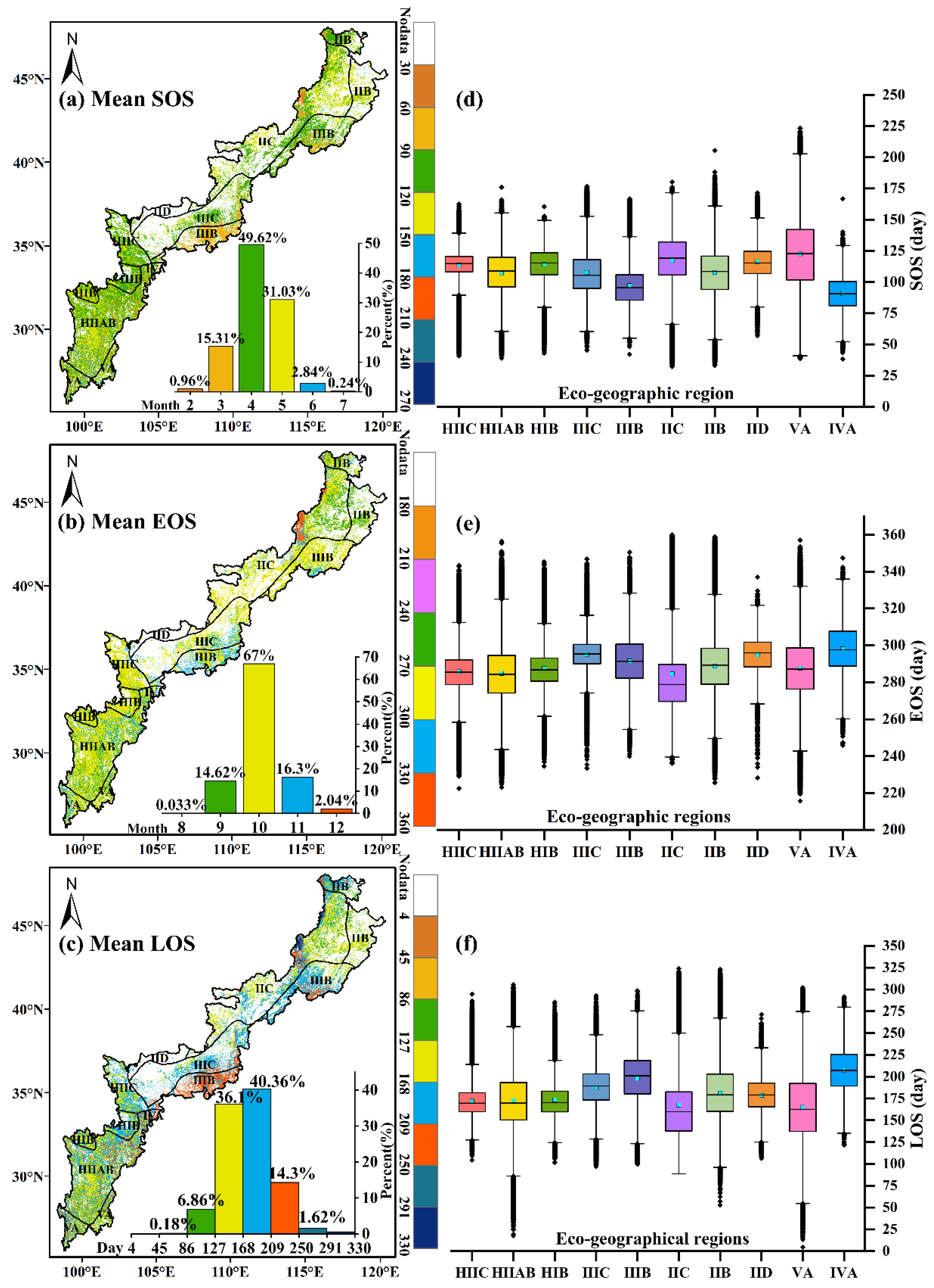
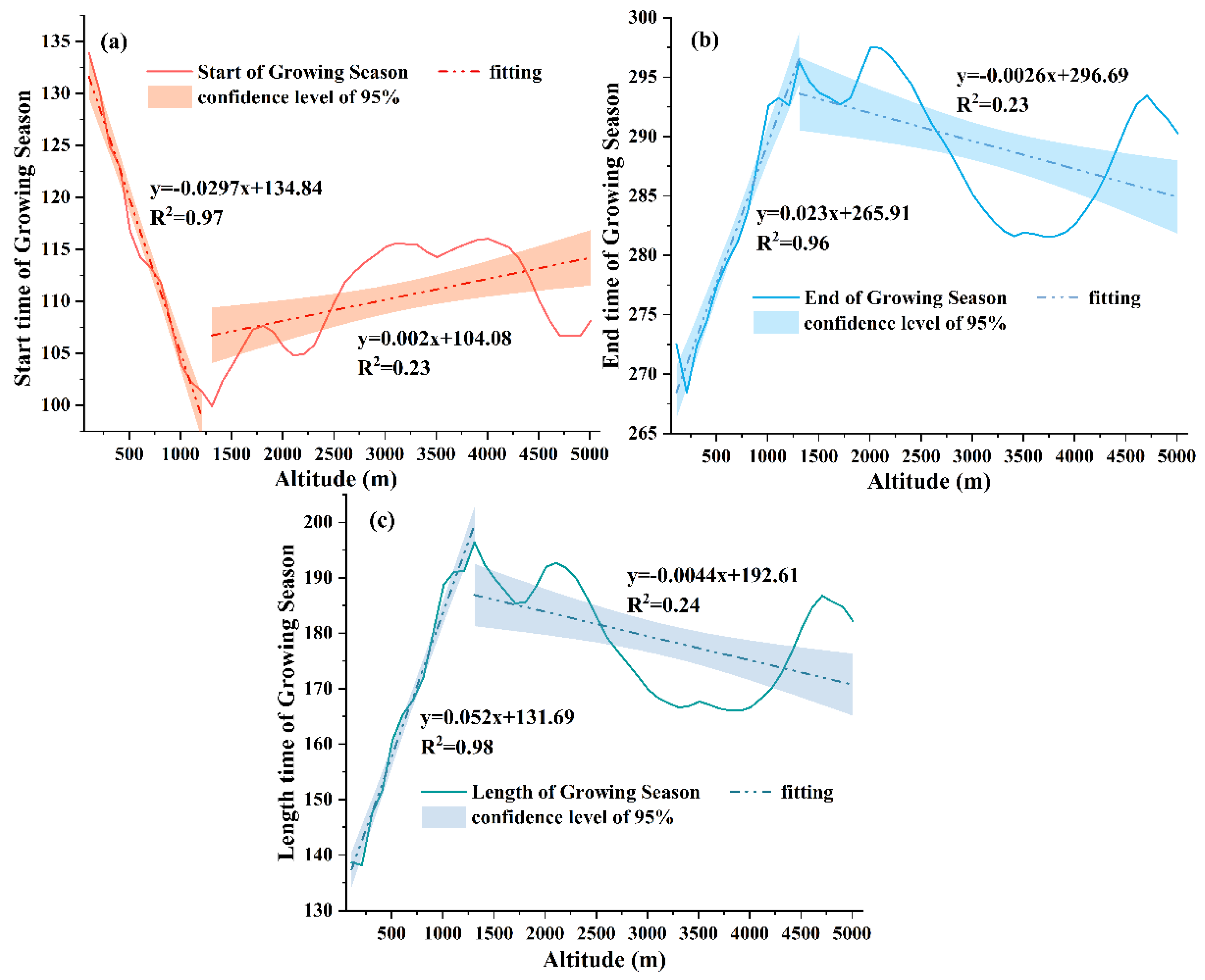
The vegetation phenology of the whole study area changed from the southern to northern latitudes in the agro-pasture ecotone, from 2000 to 2020 (Figure 3), which was due to the different geomorphologies and climates in the study area (Figure 4). As a result, the vegetation phenology presented a spatial heterogeneity and variability in different eco-geographic regions and elevations. In general, the average annual SOS in the study area was 111 d and was mainly concentrated (80.65%) from 90 d to 150 d (i.e., early April to late May) (Figure 3a). The eco-geographic regions of the study area showed a more complex, spatial variation pattern, and when the study area was divided into wet and semi-humid, semi-arid, and arid areas, according to the dry and wet zones, it was found that the mean of the SOS was ranked, from largest to smallest, as D (116 d) > C (114 d) > AB (109 d), but the pattern of the SOS was not obvious when the study area was divided, according to the temperature zones to which it belonged. At low elevations (less than 1300 m), the SOS of the study area appeared to be advanced with the increasing elevation (Figure 4e), with an advance rate of 3.0 d/100 m, but above 1500 m elevation, the SOS was found to be delayed with the increasing elevation, with a rate of 0.2 d/100 m.
Most of the study area (67%) had an EOS distribution concentrated from 270 d to 300 d (i.e., late September to late October), with an annual mean EOS of 287 d (Figure 3b). The percentage of the vegetation growing season ending in November (EOS) was 16.3%, but this was mainly distributed in the IIIB area. Overall, the spatial variability of the EOS was smaller than that of the SOS. The start of the EOS was earlier in the IIIB area, with about 37.00% of the total similar elements in September, while the start of the EOS in the central IIIB area was generally delayed until November. Except for the IIIB and IIIC areas, where the annual mean EOS was at 294 and 290 d, respectively, the mean EOS of each eco-geographic region was less variable and ranged from 270 d to 280 d. In the dry and wet zones, there was no significant difference between AB and C. However, on the temperature zones, the EOS differed more obviously, and the EOS of III and V ended the latest, at 293 d and 288 d, respectively. The EOS started earliest at low altitudes (Figure 4f), and below 1300 m, it was delayed with the increasing altitude, with a delay rate of 2.3 d/100 m. However, at higher altitudes, the EOS was advanced with the increasing altitude, and the advance rate was 0.26 d/100 m.
The LOS from 2000 to 2020 varied from 127 d to 210 d (Figure 3c), accounting for about 76.46% of the total. Most of the LOS durations of HII and HI were in this range. There were obvious spatial differences in the LOS of the study area, and the vegetation growth time in the southwest areas of VA and HIIAB ranged from 127 d to 168 d. The vegetation growth duration in the IIIB area was longer, ranging from 209 d to 250 d. The LOS duration of the IIB area was the shortest, with an average LOS of 161 days, and the distribution of the LOS in the northeast region was similar to that in the southwest region. The LOS in the AB and III regions was the longest, 176 d and 194 d, respectively. Combined with the spatial distribution of the SOS and EOS, it was found that the spatial variation of the LOS was consistent with that of the SOS. However, the variation of the LOS with altitude was found to be similar to that of the EOS. At altitudes below 1300 m, the LOS elongation rate was 5.2 d/100 m, while at higher altitudes, the LOS shortening rate was 0.44 d/100 m (Figure 4g).

3.2. Analysis of the Inter-Annual Variation in the Vegetation Phenology

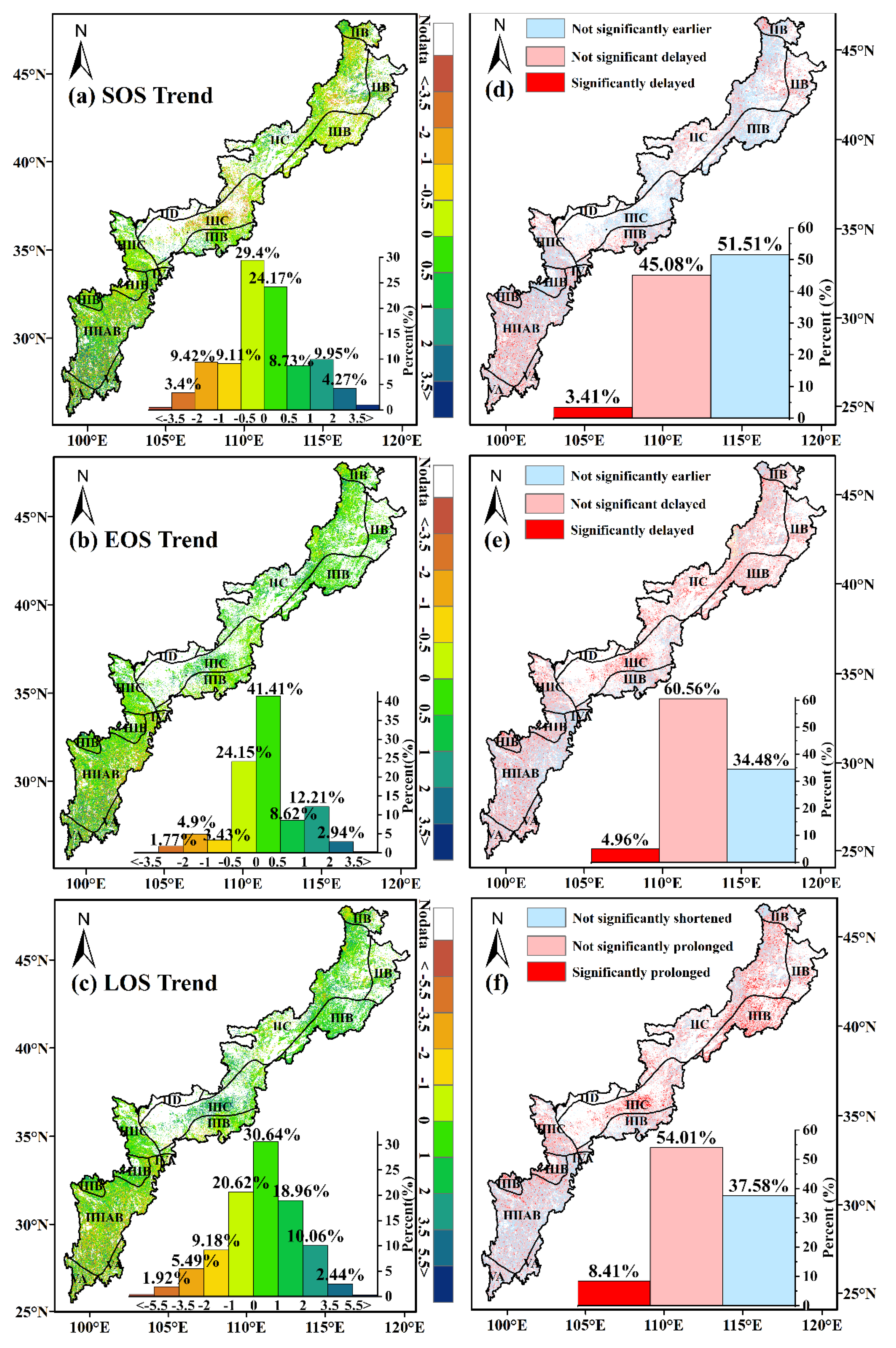
By analyzing the trends of the vegetation phenology in the agro-pasture ecotone over the past 21 years, it was found that there was no significant advance or shortening of the three phenological parameters in the study area (Figure 5). The overall SOS in the entire study area showed an advancing trend, and nearly 51.5% of the SOS showed an advancing trend (the advance rate was 0.71 d/a) (Figure 5a). For the areas with no significant advance, the areas with the largest proportions were IIIB, IIIC, and IIC (Figure 5d), accounting for 59.40%, 70.20%, and 55.22% of the area, respectively, and the advance rates were 0.42 d/a, 0.95 d/a, and 0.67 d/a (Figure 5e). A total of 48.49% of the pixels showed a trend of the SOS delay (delay rate of 0.84 d/a) (Figure 5a), of which 45.08% were not significantly delayed, indicating that the degree of the SOS delay in the study area is small, while the area with the significant delay only accounted for 3.41% of the total area, among which the HIIAB, IIB and VA regions were the regions with the most significant delay distribution, accounting for 4.33%, 7.0%, and 4.64% of the total area of these regions, respectively (Figure 5d). However, the SOS did not differ significantly in the advance and delay rates.
The EOS in the agro-pasture ecotone showed a delay trend in 65.52% of the pixels, and the change rate was above 0.6 d/a (Figure 5b). Pixels with a delay trend were found to be mainly distributed in the IIIC, IIIB, IIC, and IID regions (Figure 5e). Among these, the IIC area had the largest delay area, covering 76.10% of the area, and the delay rate was 0.5 d/a. The proportion of the areas with significant delays increased to 4.95%. Within the IIIC area of the study area, areas with a significant delay accounted for the largest proportion, at 6.80% of the total area. In general, the areas in which the delay trend passed the significance test were small, and the spatial distribution was not obvious. The vegetation EOS in 34.48% of the pixels showed an insignificant advancing trend, that is, the EOS advance in the study area was not obvious, and the degree of advance was small (Figure 5b). Region III had the smallest area of the EOS in an insignificantly advanced state, both at 27%. The leading areas were mainly in the HIIAB, HIIC, and VA regions (Figure 5e), and the leading rate in the VA region was the largest 1 d/a.
In general, the spatial distribution characteristics of the LOS change trend were found to be similar to those of the EOS (Figure 5c), i.e., the LOS as a whole, showed a lengthening trend. In the study area, 62.42% of the LOS pixels showed a lengthening trend with a change rate of 1.3 d/a, among which 32.01% of the pixels had a larger lengthening rate (>1.0 d/a) of 2.0 d/a (Figure 5f). However, most of the regions showed insignificant LOS changes, with 50.03% and 27.6% of the pixels showing insignificant lengthening and shortening trends (Figure 5c), respectively. The LOS in this region showed lengthening trends mainly in the IIIC, IIIB, and IIC regions, with 79%, 74%, and 71% of the pixels showing lengthening, respectively, with the largest lengthening rate of 1.6 d/a in the IIIC region. A total of 37.59% of the LOS showed shortening trends, with the shortening rates concentrated in the range of 0–1 d/a. The LOS shortening was mainly concentrated in the HIIAB, VA, and IVA regions, the shortening rates were 1.6 d/a, 1.9 d/a, and 1.1 d/a. The area of the whole study area with a significant extension increased to 8.41%, compared with both the SOS and EOS. The largest percentage of the area passing the significance test was located in the III area, accounting for 15.91% and 15.02% of the area, respectively. The non-significant extension was mainly distributed in the higher altitude areas, such as the HI, HII and III areas (Figure 5f).

3.3. Spatial Patterns in the Stability of the Vegetation Phenological Change

According to the coefficient of variation (Figure 6a), it was found that the mean value of the SOS coefficient of the variation in the agro-pasture ecotone over 21 years was 0.26, indicating that the stability of the SOS changes over 21 years has been poor and that the SOS has shown large fluctuations. Most of the areas in the study area (62.84%) had a medium variation intensity. Combined with the previous trend analysis, the trend of an early or delayed SOS in the agro-pasture ecotone showed fluctuating changes. The image elements in the weakly fluctuating variability accounted for only 16.19% of the total area, and they were mostly distributed in the areas of HIIC, HIB, IIC, IIB, and IIIB (Figure 6d). The mean value of the EOS coefficient of variation was 0.089 (Figure 6b), and its state of continuous variation was found to be relatively stable. The image elements with the EOS with a low degree of variation accounted for the vast majority (94.23%), and the medium variation was mainly distributed in the VA area (Figure 6e), but there was no strong variation, which indicates the EOS on a large scale. The spatial distribution of the coefficient of variation of the LOS was similar to that of the SOS, with a mean coefficient of variation of 0.21 (Figure 6c), and overall medium variation intensity, but there were more pixels with a weak variation than in the SOS, accounting for 26.30% of the total area, and most of the pixels in the HIIC and IIIB regions showed a weak variation. The HIIC and IIIB areas had a weak variation, that is, the trend of the LOS lengthening in this area was relatively stable and did not show a large volatility over the 21 years. The proportion of the strong variation has decreased, by about 11.07%, and the vast majority of the areas with strong variation were found to be distributed in the VA and HIIAB areas (Figure 6f).

3.4. The Relationship between the Vegetation Phenology and the Climate

3.4.1. Precipitation and Temperature Response to the SOS

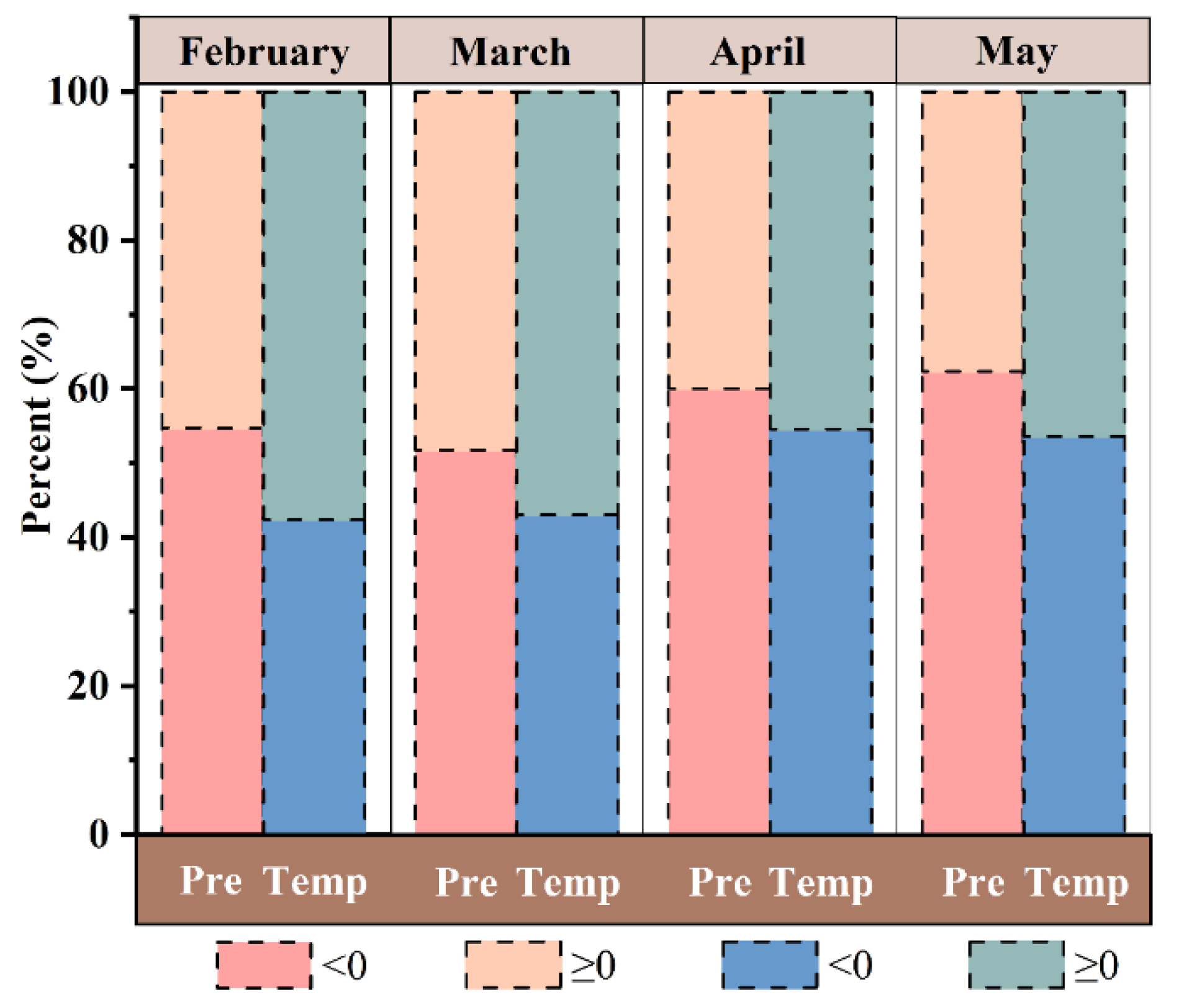
For the whole study area, the percentage of the mean precipitation, from February to May, which is negatively correlated with the SOS, increased with the increase in months (Figure 7), but the effect of the precipitation on the SOS varied at different times in the same area, which was also reflected in the effect of the temperature on the SOS. The bias correlation coefficients between the SOS and mean precipitation, from February to May, were mainly negative. This indicates that as precipitation increases, the SOS also advances. The largest effect of the precipitation on the SOS occurred in May, with 7.66% of the pixels showing a significant negative correlation. The bias correlation coefficients between the mean temperature, from February to March, and the SOS were mainly positive (Figure 7), while the bias correlation coefficients with the mean temperature in April and May were mostly negative. This indicates that the SOS was delayed in most areas of the study area in April and May as the temperature decreased during those months. In terms of significance levels, the SOS had the highest number of significant-like points (6.53%) for the bias correlation coefficient with a mean precipitation in May, indicating that the vegetation SOS was influenced by the mean precipitation in May in more areas. The effect of the temperature on the SOS, was greatest in March, with a negative correlation coefficient of only 5.29%.
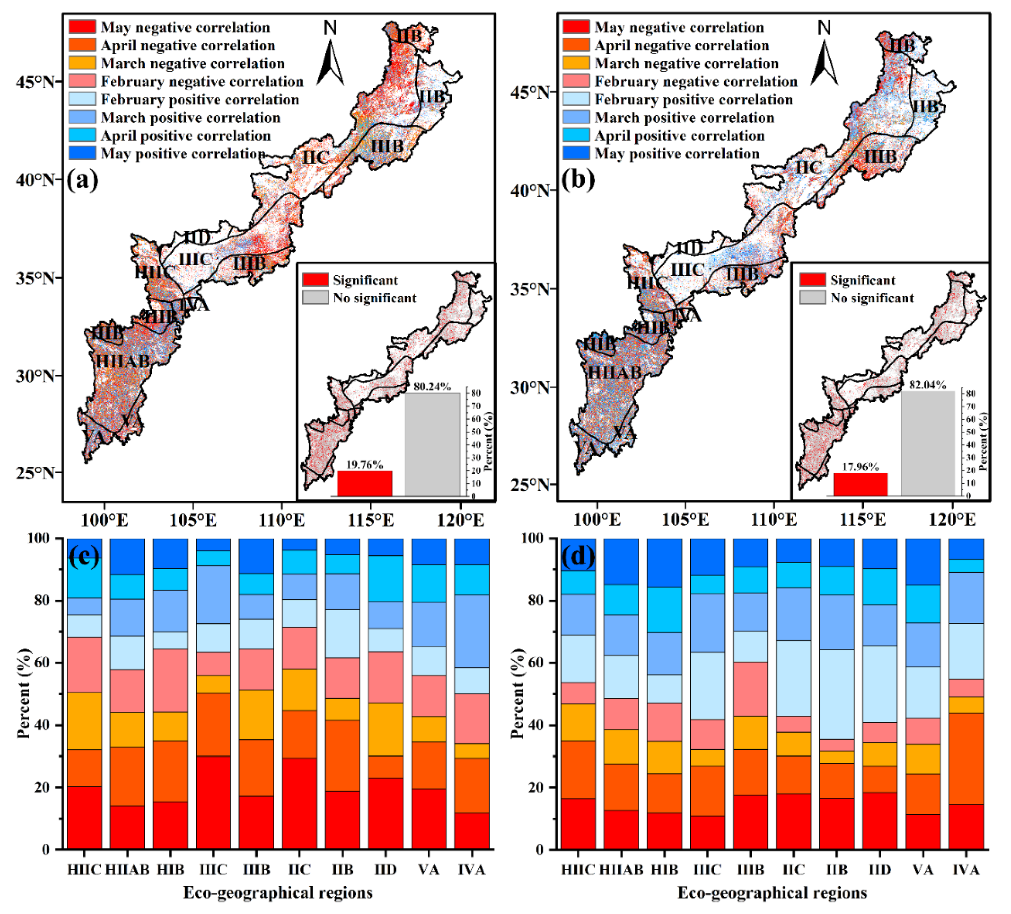
In terms of the effect of precipitation on the SOS, most of the study area (63.36%) had a negative correlation (Figure 8a,c). This indicates that, as precipitation decreased in the corresponding areas and months, the SOS was subsequently delayed. In 25.41% and 28.47% of the pixels, the SOS was mainly affected by precipitation in April and May, and the effect was predominantly negative. The bias correlation coefficients of precipitation on the SOS in the corresponding months were large, and the absolute values were between 0.4 and 0.6. In terms of wet and dry zones, the percentage of the negative correlation between the SOS and precipitation in area A/B (59.01%) was significantly smaller than that in area C/D (66.67%). In terms of significance levels, 19.79% of the image elements passed the significance test, but more image elements passed the significance test in the A/B area (19.97%) than in the C/D area (19.50%). In terms of temperature, the effect of temperature on the SOS was most pronounced in February and May (26.61% and 25.38%), but there was spatial variability in their distributions (Figure 8b,d). The effect of temperature on the SOS in February and March was mainly positive, which indicated that the increase in temperature in February and March would delay the SOS. In contrast, the effect of temperature on the SOS in April and May was predominantly negative. In terms of the temperature areas (Table 1), the response of the effect of temperature on the SOS varied across the temperature areas. In general, the percentage of the negative correlation of the temperature on the SOS decreased as the number of days with temperature areas greater than 10 °C and the number of days with an accumulation temperature greater than 10 °C, increased for the same dry and wet conditions. The bias correlation coefficient of the temperature to the SOS, passed the significance test for fewer image elements than the precipitation, with about 17.96% passing the significance test.

3.4.2. Impact of the Precipitation and Temperature on the EOS

Compared with the SOS, the spatial and temporal variation of precipitation had a more significant effect on the EOS. The EOS was positively correlated with the mean precipitation, from August to November, in most areas of the study area (Figure 9). Precipitation in September had the greatest effect on the EOS. A total of 60.76% of the areas were positively correlated, and 7.32% of the pixels were significantly affected, indicating that the EOS was delayed in most areas, as precipitation increased. The partial correlation coefficients between the EOS and mean temperature in August, October, and November were mostly positive (Figure 9), and the partial correlation coefficients with the mean temperature in September were mostly negative. The correlation coefficients were mostly negative, and there were limited correlations (positive and negative) between the EOS and temperature. However, the response of the EOS to temperature varied with the month in each region. In Northeast China, the EOS was mostly negatively correlated with temperature in October and November, while it was mostly positively correlated in August and September.
In the case of the greatest influence of precipitation, the EOS was mainly influenced by the positive influence of the average precipitation (60.91%), which indicates that the EOS had advanced with the increase in precipitation in the corresponding month (Figure 10a,c). In general, there was no significant difference in the percentage of precipitation playing an influential role on the EOS in each month. However, the percentage of the degree of impact of the precipitation on the EOS varies from month to month in different regions, and the precipitation in September has the largest impact on the EOS in most regions. The negative correlation of the precipitation on the EOS was greater in region C/D (68.09%) than in region A/B (58.08%). In terms of its significance, the percentage of image elements that pass the significance test was 21.56%. A total of 22.23% passed the significance test in the C/D region, compared to 21.53% in the A/B region. As far as temperature is concerned, the image elements with a positive effect on the EOS accounted for 49.84% of the total area (Figure 10b,d). The most image points (29.34%) had the main temperature effect on the EOS in September, and most of them were positive, indicating that the increase in temperature in September can delay the EOS. In general, the proportion of the negative correlations of the temperature on the EOS decreased as the accumulated temperature increased in the temperature zones, while the dry and wet conditions remained the same. With the maximum temperature effect, its partial correlation coefficient with the EOS passed the significance test, but to a smaller extent than precipitation (19.07%).

4. Discussion

Since the 1960s, climate change in China has been characterized by significant warming [20]. As the region where agriculture and animal husbandry are interspersed in China, combined with the complex local eco-geographical regional systems, the vegetation phenology of the agro-pasture ecotone is particularly sensitive to global climate change. Spatially, the SOS of the study area showed high ends and a low middle, which is identical with the results reported by Hou et al. [40]. In general, it is early in the northeast and late in the southwest, which is similar to the results of Yang et al. [63] for the vegetation phenology changes in China, from 1982 to 2010. The trends of vegetation phenology in the agro-pasture ecotone over the past 21 years are consistent with the results of Piao et al. [48] for the temperate zone of China—the SOS is 0.79 d earlier and the EOS is 0.37 d later for the whole region, but the degree of the vegetation phenology variation in the different eco-geographical systems shows some difference. In different dry and wet zones, the advance of the SOS was C/D (0.6 d) < A/B (0.9 d) and the delay of the EOS was C/D (0.18 d) < A/B (0.53 d). This is consistent with most of the studies by Tao et al. [22] regarding the positive effect of precipitation on the vegetation phenology [30,31]. However, the heterogeneity of the SOS and the EOS was more pronounced in the temperature band. In general, the higher the cumulus temperature, the more pronounced the overall tendency of the SOS and the EOS exhibited earlier or delayed, also contributing to the prolongation of the LOS, which is consistent with other studies [25,31]. This illustrates that the vegetation growth was favored under the suitable precipitation and temperature [32].
“The Hopkins bioclimatic law” states that the spring phenology of vegetation is steadily delayed with the increasing latitude and elevation [64]. This is somewhat different from the results of our study. In this study, we found that the change in the vegetation phenology was segmented with the increasing altitude. Firstly, in the low elevation area (less than 1300 m), its SOS appeared to be delayed with the elevation, the EOS was advanced, and the LOS was gradually shortened. This may be due to the fact that most of the low elevation areas are at high latitudes (i.e., Northeast China). The air temperature in this region is influenced by the Siberian cold current, and the air temperature drops faster in spring and autumn than in the high altitudes of Southwest China [65,66]. Therefore, the SOS is delayed while the EOS is advanced to avoid frost damage, causing the LOS to be shortened. This finding is consistent with the results of Xia et al. at lower elevations [67]. Secondly, the fluctuating changes in the SOS, EOS, and LOS were observed at high altitudes, but the SOS still showed a moderate upward trend, while the EOS, and LOS showed a moderate downward trend. According to Piao et al. [23], since the air temperature is relatively low at high altitudes, it could delay vegetation growth and accelerate leaf senescence. However, this correlation was found to be weak, based on the actual area of this study, and the air temperature may not be the main driver of the vegetation growth at high altitudes. In this study, we found that the high elevation areas are all in the A/B region, with a relatively high precipitation, which may encourage the vegetation growth. Furthermore, an interesting phenomenon that the SOS was significantly later in the northeastern part of the study area than in the southwestern part, while the EOS was earlier than in the southwestern part [68]. This difference may be due to the cultivated vegetation and the predominantly herbaceous vegetation in the northeast, while the southwest is characterized by tall forests and shrublands. Walther et al. [1] observed that the cultivated vegetation and herbaceous plants are more sensitive to the changes in temperature than other types of vegetation. Thus, when the cold season is earlier in the northeast than in the southwest, its vegetation phenology is more significant earlier or later than that in the southwest.
Numerous surface and remote sensing observations suggest that the SOS is significantly advanced, due to global warming [69,70,71]. However, according to the results of this paper, there is a large spatial variation in the effect of the temperature on the SOS. In the C/D region, the temperature showed a more positive correlation to the SOS, i.e., an increase in temperature instead of a delayed SOS. This is similar to the findings of some recent studies—as temperatures continue to increase, the sensitivity of the SOS to temperature gradually decreases, which can even lead to a delayed SOS [17]. The SOS in the study area was most influenced by the average precipitation in April and May, which mainly showed a negative correlation, i.e., a reduced precipitation in spring led to a delay in the spring phenology. Compared with area A/B, the local SOS was significantly earlier in area C/D with the increase in precipitation. These findings are similar with the conclusions of Kang et al., Ge et al., and Zeng et al. [34,72,73]. They discovered that the increase in temperature can allow the vegetation to obtain sufficient light and suitable growing temperatures in some areas, and this can improve its growth rate and advance the phenological period [34,73]. In some C/D areas, the increase in temperature can lead to a decrease in soil moisture in the area, affecting the pre-season water accumulation and delaying the phenological period instead. Several studies have shown that temperature is the main factor that nonlinearly affects the phenological changes [74,75]. Moreover, precipitation can significantly affect the phenology, when it becomes a stressor. Insufficient water availability in C/D areas can inhibit vegetation light and heat use. However, the effect of precipitation on the vegetation phenology in the C/D region needs further study. On the one hand, water resources available for vegetation can be provided, not only by precipitation, but also related to the soil water content and local groundwater [35]. On the other hand, Yang et al. suggested that the response of the vegetation phenology to precipitation is complex, and there may be a temporal continuum or lag in the effect on it [63].
In general, temperature and precipitation are positively correlated with the EOS in all months except September when the temperature has a negative effect on the EOS, i.e., an increase in the temperature in that month can advance the EOS [21]. The possible reason for this is that the highest summer temperatures are in July and August, and the temperature at this stage is in line with the growth pattern of vegetation [76]. When the temperature rises in September, it will intensify the respiration of plants and inhibit photosynthesis, resulting in a lower enzyme activity in plants and evaporation of water, which will cause vegetation to enter dormancy earlier [76,77]. Moreover, among them, precipitation and temperature in September have the greatest impact on the EOS [14]. Although according to the results of previous studies, warming is the main factor that causes the delay of the EOS, some researchers believe that the effect of temperature on the EOS is somewhat overestimated. In the present study, precipitation also had a very important effect on the EOS. The effect of temperature on the EOS varied slightly in different temperature zones, while precipitation had a more profound effect, especially in the A/B and C/D regions. Although we did not analyze the bias correlation between temperature and precipitation for the LOS, previous studies have demonstrated that the effects of precipitation and temperature on the SOS and EOS in each month also act on the LOS [28,78]. Therefore, suitable temperature and precipitation positively affect plant growth and promote a longer growing season [71].

5. Conclusions

In this study, MODIS EVI time series data, from 2000 to 2020, were used to investigate the spatial variation characteristics of the vegetation phenology in different eco-geographic regions in the China’s agro-pasture ecotone, over 21 years. This study also analyzed the response of the vegetation phenology to climate change in the context of global climate change. The main conclusions are as follows. (1) The SOS of the vegetation in China’s agro-pastoral zone, is mainly concentrated, from 90 to 150 d, the EOS is mainly concentrated, from 270 to 300 d, and LOS is concentrated, from 127 to 210 d. Meanwhile, the concentration degree of the phenological date varies in the different ecological-geographical zones, and the dates of the vegetation phenology appear to be advanced or delayed with the different eco-geographic regions. This mainly occurred in the dry and wet zones, and was less pronounced in the temperate zones. (2) In the whole region, the SOS showed an overall trend of advancement, the EOS showed an overall delay, and the LOS was prolonged. The physical changes in the different landscape zones were found to be spatially heterogeneous. However, when the elevation exceeded a certain height, and with increases in elevation, the phenological trend became less obvious. (3) The response of vegetation phenology to the climatic factors is very complex. The SOS was found to be mainly negatively correlated with the mean precipitation, from February to May. In the C/D region, an increase in precipitation can lead to the SOS advancement in most regions. However, the relationship between the temperature and the SOS is not significant, compared with the precipitation. The EOS was mainly positively influenced by the increased precipitation in September. The effect of precipitation on the EOS was greater in region C/D than in region A/B. The results suggest that the phenology is very sensitive to climate and that different ecological geographies may have different phenology types. These findings may help reveal regional microclimate phenology patterns and contribute to understanding the potential long-term effects of climate change on the phenology.
The accuracy of the analysis of the effects of climate change on the vegetation phenology under this condition may be compromised, owing to the limitations of the unnatural vegetation cover types and data availability. To overcome these shortcomings, we aim to integrate a series of products that can reflect the dynamic changes of vegetation, improve the temporal and spatial resolution of the products, or explore how the accuracy of their extracted phenology can be studied, using the same method, based on different data sources. In addition, when discussing the influencing factors of the vegetation phenology changes, in addition to the influence of precipitation and temperature on the vegetation phenology in the region, other environmental factors, such as photoperiod, radiation intensity, carbon concentration, etc. should not be neglected [55,64]. However, behind the effects caused by these factors is a complex systemic vegetation ecology, which involves the whole process of vegetation growth. Therefore, we will incorporate all of the influencing factors into the analysis in the future, and establish a numerical model of vegetation phenology and each factor to make a more accurate estimation and prediction of the vegetation phenology changes.

Author Contributions

Conceptualization, J.F., Q.Y., J.N. and X.W.; methodology, J.F., J.M., Q.Y. and X.W.; software, J.M. and J.F.; validation, J.F., J.N. and J.M.; formal analysis, J.F.; investigation, J.F. and J.M.; resources, Q.Y. and X.W.; data curation, J.F., J.M. and J.N.; writing—review and editing, J.F., J.M. and J.N; visualization, J.F. and J.M.; supervision, Q.Y.; project administration, Q.Y.; funding acquisition, Q.Y. All authors have read and agreed to the published version of the manuscript.

Funding

This study was supported by the Strategic Priority Research Program of the Chinese Academy of Sciences (NO. XDA19030500) and the Foundation of Social Science and Humanity, China Ministry of Education (NO. 22YJCZH130).

Institutional Review Board Statement

Not applicable.

Data Availability Statement

The data used in this study were obtained from the following platforms: Geospatial Data Cloud for the digital elevation data (http://www.gscloud.cn/ (accessed on 5 March 2022)), GLOBELAND30 for the land cover data (http://www.globallandcover.com/ (accessed on 5 March 2022)), the LAADS of NASA for the MODIS products (https://modis.gsfc.nasa.gov/ (accessed on 30 September 2021)), Notion Earth System Science Data Center for the meteorological data and eco-geographical data (http://www.geodata.cn (accessed on 12 April 2022)).

Acknowledgments

We acknowledge the data support from “National Earth System Science Data Center, National Science & Technology Infrastructure of China. (http://www.geodata.cn (accessed on 12 April 2022))”.

Conflicts of Interest

The authors declare no conflict of interest.

References

  1. Walther, G.R.; Post, E.; Convey, P.; Menzel, A.; Parmesan, C.; Beebee, T.J.; Fromentin, J.M.; Hoegh-Guldberg, O.; Bairlein, F. Ecological responses to recent climate change. Nature 2002, 416, 389–395. [Google Scholar] [CrossRef]
  2. White, M.A.; De Beurs, K.M.; Didan, K.; Inouye, D.W.; Richardson, A.D.; Jensen, O.P.; O’Keefe, J.; Zhang, G.; Nemani, R.R.; van Leeuwen, W.J.D.; et al. Intercomparison, interpretation, and assessment of spring phenology in North America estimated from remote sensing for 1982–2006. Glob. Chang. Biol. 2009, 15, 2335–2359. [Google Scholar] [CrossRef]
  3. Ge, Q.; Dai, J.; Zheng, J. The progress of phenology studies and challenges to modern phenology research in China. Bull. Chin. Acad. Sci. 2010, 25, 310–316. [Google Scholar]
  4. Beaubien, E.G.; Freeland, H.J. Spring phenology trends in Alberta, Canada: Links to ocean temperature. Int. J. Biometeorol. 2000, 44, 53–59. [Google Scholar] [CrossRef] [PubMed]
  5. Flynn, D.F.B.; Wolkovich, E.M. Temperature and photoperiod drive spring phenology across all species in a temperate forest community. New Phytol. 2018, 219, 1353–1362. [Google Scholar] [CrossRef] [PubMed] [Green Version]
  6. McCarthy, J.J.; Canziani, O.F.; Leary, N.A.; Dokken, D.J.; White, K.S. Climate Change 2001: Impacts, Adaptation, and Vulnerability: Contribution of Working Group II to the Third Assessment Report of the Intergovernmental Panel on Climate Change; Cambridge University Press: Cambridge, UK, 2001; Volume 2. [Google Scholar]
  7. Richardson, A.D.; Keenan, T.F.; Migliavacca, M.; Ryu, Y.; Sonnentag, O.; Toomey, M. Climate change, phenology, and phenological control of vegetation feedbacks to the climate system. Agric. For. Meteorol. 2013, 169, 156–173. [Google Scholar] [CrossRef]
  8. Piao, S.; Liu, Q.; Chen, A.; Janssens, I.A.; Fu, Y.; Dai, J.; Liu, L.; Lian, X.; Shen, M.; Zhu, X. Plant phenology and global climate change: Current progresses and challenges. Glob. Chang. Biol. 2019, 25, 1922–1940. [Google Scholar] [CrossRef]
  9. Studer, S.; Stockli, R.; Appenzeller, C.; Vidale, P.L. A comparative study of satellite and ground-based phenology. Int. J. Biometeorol. 2007, 51, 405–414. [Google Scholar] [CrossRef] [Green Version]
  10. Cleland, E.E.; Chuine, I.; Menzel, A.; Mooney, H.A.; Schwartz, M.D. Shifting plant phenology in response to global change. Trends. Ecol. Evol. 2007, 22, 357–365. [Google Scholar] [CrossRef]
  11. Zhu, W.; Tian, H.; Xu, X.; Pan, Y.; Chen, G.; Lin, W. Extension of the growing season due to delayed autumn over mid and high latitudes in North America during 1982–2006. Glob. Ecol. Biogeogr. 2012, 21, 260–271. [Google Scholar] [CrossRef]
  12. Mackay, A. Climate change 2007: Impacts, adaptation and vulnerability. Contribution of Working Group II to the fourth assessment report of the Intergovernmental Panel on Climate Change. J. Environ. Qual. 2008, 37, 2407. [Google Scholar] [CrossRef]
  13. Rosenzweig, C.; Casassa, G.; Karoly, D.J.; Imeson, A.; Liu, C.; Menzel, A.; Rawlins, S.; Root, T.L.; Seguin, B.; Tryjanowski, P. Assessment of observed changes and responses in natural and managed systems. Disasters 2007, 79–131. [Google Scholar]
  14. Meng, L.; Zhou, Y.; Gu, L.; Richardson, A.D.; Penuelas, J.; Fu, Y.; Wang, Y.; Asrar, G.R.; De Boeck, H.J.; Mao, J.; et al. Photoperiod decelerates the advance of spring phenology of six deciduous tree species under climate warming. Glob. Chang. Biol. 2021, 27, 2914–2927. [Google Scholar] [CrossRef] [PubMed]
  15. Wu, X.; Liu, H. Consistent shifts in spring vegetation green-up date across temperate biomes in China, 1982–2006. Glob. Chang. Biol. 2013, 19, 870–880. [Google Scholar] [CrossRef] [PubMed]
  16. Myneni, R.B.; Keeling, C.; Tucker, C.J.; Asrar, G.; Nemani, R.R. Increased plant growth in the northern high latitudes from 1981 to 1991. Nature 1997, 386, 698–702. [Google Scholar] [CrossRef]
  17. Fu, Y.H.; Piao, S.; Op de Beeck, M.; Cong, N.; Zhao, H.; Zhang, Y.; Menzel, A.; Janssens, I.A. Recent spring phenology shifts in western Central Europe based on multiscale observations. Glob. Ecol. Biogeogr. 2014, 23, 1255–1263. [Google Scholar] [CrossRef]
  18. Peñuelas, J.; Filella, I. Responses to a warming world. Science 2001, 294, 793–795. [Google Scholar] [CrossRef]
  19. IPCC. Climate Change 2007: Synthesis Report; IPCC: Geneva, Switzerland, 2007. [Google Scholar]
  20. Yang, Q.; Zheng, X.; He, L.-H. Spatial-temporal shift for major boundary of climate regionalization based on meteorological data stimulated by HadCM3 during from 1950–2059 in China. Arid. Land Geogr. 2017, 40, 17–25. [Google Scholar]
  21. Fu, Y.H.; Zhao, H.; Piao, S.; Peaucelle, M.; Peng, S.; Zhou, G.; Ciais, P.; Huang, M.; Menzel, A.; Peñuelas, J. Declining global warming effects on the phenology of spring leaf unfolding. Nature 2015, 526, 104–107. [Google Scholar] [CrossRef] [Green Version]
  22. Tao, Z.; Wang, H.; Liu, Y.; Xu, Y.; Dai, J. Phenological response of different vegetation types to temperature and precipitation variations in northern China during 1982–2012. Int. J. Remote Sens. 2017, 38, 3236–3252. [Google Scholar] [CrossRef]
  23. Piao, S.; Cui, M.; Chen, A.; Wang, X.; Ciais, P.; Liu, J.; Tang, Y. Altitude and temperature dependence of change in the spring vegetation green-up date from 1982 to 2006 in the Qinghai-Xizang Plateau. Agric. For. Meteorol. 2011, 151, 1599–1608. [Google Scholar] [CrossRef]
  24. Steltzer, H.; Post, E. Seasons and life cycles. Science 2009, 324, 886–887. [Google Scholar] [CrossRef] [PubMed]
  25. Mo, F.; Zhao, H.; Wang, J.; Qiang, S.; Zhou, H.; Wang, S.; Xiong, Y. The key issues on plant phenology under global change. Shengtai Xuebao/Acta Ecol. Sin. 2011, 31, 2593–2601. [Google Scholar]
  26. Chidumayo, E. Climate and phenology of savanna vegetation in southern Africa. J. Veg. Sci. 2001, 12, 347. [Google Scholar] [CrossRef]
  27. Piao, S.; Friedlingstein, P.; Ciais, P.; Viovy, N.; Demarty, J. Growing season extension and its impact on terrestrial carbon cycle in the Northern Hemisphere over the past 2 decades. Glob. Biogeochem. Cycles 2007, 21. [Google Scholar] [CrossRef]
  28. Jeong, S.J.; Ho, C.H.; Gim, H.J.; Brown, M.E. Phenology shifts at start vs. end of growing season in temperate vegetation over the Northern Hemisphere for the period 1982–2008. Glob. Chang. Biol. 2011, 17, 2385–2399. [Google Scholar] [CrossRef]
  29. Marchin, R.M.; Salk, C.F.; Hoffmann, W.A.; Dunn, R.R. Temperature alone does not explain phenological variation of diverse temperate plants under experimental warming. Glob. Chang. Biol. 2015, 21, 3138–3151. [Google Scholar] [CrossRef]
  30. Zhang, X.; Friedl, M.A.; Schaaf, C.B.; Strahler, A.H.; Liu, Z. Monitoring the response of vegetation phenology to precipitation in Africa by coupling MODIS and TRMM instruments. J. Geophys. Res. Atmos. 2005, 110. [Google Scholar] [CrossRef]
  31. Yun, J.; Jeong, S.J.; Ho, C.H.; Park, C.E.; Park, H.; Kim, J. Influence of winter precipitation on spring phenology in boreal forests. Glob. Chang. Biol. 2018, 24, 5176–5187. [Google Scholar] [CrossRef]
  32. Shen, M.; Piao, S.; Cong, N.; Zhang, G.; Jassens, I.A. Precipitation impacts on vegetation spring phenology on the Tibetan Plateau. Glob. Chang. Biol. 2015, 21, 3647–3656. [Google Scholar] [CrossRef] [Green Version]
  33. Wu, L.; Ma, X.; Dou, X.; Zhu, J.; Zhao, C. Impacts of climate change on vegetation phenology and net primary productivity in arid Central Asia. Sci. Total Environ. 2021, 796, 149055. [Google Scholar] [CrossRef] [PubMed]
  34. Ge, W.; Han, J.; Zhang, D.; Wang, F. Divergent impacts of droughts on vegetation phenology and productivity in the Yungui Plateau, southwest China. Ecol. Indic. 2021, 127, 107743. [Google Scholar] [CrossRef]
  35. Liu, X.; Chen, Y.; Li, Z.; Li, Y.; Zhang, Q.; Zan, M. Driving Forces of the Changes in Vegetation Phenology in the Qinghai–Tibet Plateau. Remote Sens. 2021, 13, 4952. [Google Scholar] [CrossRef]
  36. Chen, X.; Pan, X.; Wei, Y. Climate Change and its Impacts ori Herbaceous Plant Phenology in Farming-Pastoral Mixed Ecotopes. Chin. J. Agrometeorol. 2006, 14–17. [Google Scholar]
  37. Li, D.; Lu, L. Climate Characters and Evolution of Agricultural and Pasturing Interlaced Zone in China. J. Desert Res. 2002, 22, 483. [Google Scholar]
  38. Cheng, X. Frontier issue of modern ecology in the study of ecotone between agriculture and animal husbandry. Resour. Sci. 1999, 21, 3–10. [Google Scholar]
  39. Liu, H.; Wang, Y.; Dou, X.; Xu, M.; Wang, K. Progress and Perspective of Agro-pasturage Ecotone. Acta Ecol. Sin. 2009, 29, 4420–4425. [Google Scholar]
  40. Hou, X.; Niu, Z.; Gao, S.; Huang, N. Monitoring vegetation phenology in farming-pastoral zone using SPOT-VGT NDVI data. Trans. Chin. Soc. Agric. Eng. 2013, 29, 142–150+294. [Google Scholar]
  41. Wu, G. Research Advance on the Farming-grazing Transitional Zone in China. J. Sichuan Norm. Univ. (Nat. Sci.) 2003, 26, 108–110. [Google Scholar]
  42. Li, X.; Yang, L.; Tian, W.; Xu, X.; He, C. Land use and land cover change in agro-pastoral ecotone in Northern China: A review. Chin. J. Appl. Ecol. 2018, 29, 3487–3495. [Google Scholar] [CrossRef]
  43. Cihlar, J.; Ly, H.; Li, Z.; Chen, J.; Pokrant, H.; Huang, F. Multitemporal, multichannel AVHRR data sets for land biosphere studies—Artifacts and corrections. Remote Sens. Environ. 1997, 60, 35–57. [Google Scholar] [CrossRef]
  44. Li, H.; Jia, Y.; Ma, M. Application. Reconstruction of temporal NDVI dataset: Evaluation and case study. J. Remote Sens. Technol. 2010, 24, 596–602. [Google Scholar]
  45. Madden, H.H. Comments on the Savitzky-Golay convolution method for least-squares-fit smoothing and differentiation of digital data. Anal. Chem. 1978, 50, 1383–1386. [Google Scholar] [CrossRef]
  46. Chen, J.; Jönsson, P.; Tamura, M.; Gu, Z.; Matsushita, B.; Eklundh, L. A simple method for reconstructing a high-quality NDVI time-series data set based on the Savitzky–Golay filter. Remote Sens. Environ. 2004, 91, 332–344. [Google Scholar] [CrossRef]
  47. Savitzky, A.; Golay, M.J. Smoothing and differentiation of data by simplified least squares procedures. Anal. Chem. 1964, 36, 1627–1639. [Google Scholar] [CrossRef]
  48. Piao, S.L.; Fang, J.Y.; Zhou, L.M.; Ciais, P.; Zhu, B. Variations in satellite-derived phenology in China’s temperate vegetation. Glob. Chang. Biol. 2006, 12, 672–685. [Google Scholar] [CrossRef]
  49. Peng, S.; Ding, Y.; Wen, Z.; Chen, Y.; Cao, Y.; Ren, J. Spatiotemporal change and trend analysis of potential evapotranspiration over the Loess Plateau of China during 2011–2100. Agric. For. Meteorol. 2017, 233, 183–194. [Google Scholar] [CrossRef] [Green Version]
  50. Ding, Y.; Peng, S. Spatiotemporal trends and attribution of drought across China from 1901–2100. Sustainability 2020, 12, 477. [Google Scholar] [CrossRef] [Green Version]
  51. Zheng, D. Research on Eco-Geographical Region Systems in China; The Commercial Press: Beijing, China, 2008. [Google Scholar]
  52. Jun, C.; Ban, Y.; Li, S. Open access to Earth land-cover map. Nature 2014, 514, 434. [Google Scholar] [CrossRef] [Green Version]
  53. Chen, J.; Chen, J.; Liao, A. Remote Sensing Mapping of Global Land Cover; Science Press: Beijing, China, 2016. [Google Scholar]
  54. Liu, Q.; Fu, Y.H.; Zeng, Z.; Huang, M.; Li, X.; Piao, S. Temperature, precipitation, and insolation effects on autumn vegetation phenology in temperate China. Glob. Chang. Biol. 2016, 22, 644–655. [Google Scholar] [CrossRef]
  55. Zhang, G.L.; Zhang, Y.J.; Dong, J.W.; Xiao, X.M. Green-up dates in the Tibetan Plateau have continuously advanced from 1982 to 2011. Proc. Natl. Acad. Sci. USA 2013, 110, 4309–4314. [Google Scholar] [CrossRef] [PubMed]
  56. Han, H.; Bai, J.; Ma, G.; Yan, J. Vegetation phenological changes in multiple landforms and responses to climate change. ISPRS Int. J. Geo-Inf. 2020, 9, 111. [Google Scholar] [CrossRef] [Green Version]
  57. Sen, P.K. Estimates of the regression coefficient based on Kendall’s tau. J. Am. Stat. Assoc. 1968, 63, 1379–1389. [Google Scholar] [CrossRef]
  58. Yin, H.; Li, Z.; Wang, Y.; Cai, F. Assessment of desertification using time series analysis of hyper-temporal vegetation indicator in Inner Mongolia. Acta Geogr. Sin. 2011, 66, 653–661. [Google Scholar]
  59. Mann, H.B. Nonparametric tests against trend. Econom. J. Econom. Soc. 1945, 13, 245–259. [Google Scholar] [CrossRef]
  60. Kendall, M.G. Rank Correlation Methods, 4th ed.; Charles Griffin: London, UK, 1975. [Google Scholar]
  61. Le, W.; Dedi, L.; Tianyuan, L. Trend Analysis of Precipitation in Beijiang River Basin Based on Multivariate Mann-Kendall Test. J. China Hydrol. 2015, 35, 85–90. [Google Scholar]
  62. Wang, D.; Formica, M.K.; Liu, S. Nonparametric interval estimators for the coefficient of variation. Int. J. Biostat. 2018, 14. [Google Scholar] [CrossRef]
  63. Yang, Y.; Guan, H.; Shen, M.; Liang, W.; Jiang, L. Changes in autumn vegetation dormancy onset date and the climate controls across temperate ecosystems in China from 1982 to 2010. Glob. Chang. Biol. 2015, 21, 652–665. [Google Scholar] [CrossRef]
  64. Hopkins, A.D. The bioclimatic law. J. Wash. Acad. Sci. 1920, 10, 34–40. [Google Scholar]
  65. Peng, S.; Piao, S.; Ciais, P.; Myneni, R.B.; Chen, A.; Chevallier, F.; Dolman, A.J.; Janssens, I.A.; Penuelas, J.; Zhang, G.J.N. Asymmetric effects of daytime and night-time warming on Northern Hemisphere vegetation. Nature 2013, 501, 88–92. [Google Scholar] [CrossRef]
  66. Wang, S.; Yang, B.; Yang, Q.; Lu, L.; Wang, X.; Peng, Y. Temporal trends and spatial variability of vegetation phenology over the Northern Hemisphere during 1982–2012. PLoS ONE 2016, 11, e0157134. [Google Scholar] [CrossRef] [PubMed] [Green Version]
  67. Xia, H.; Xia, H.; Zhao, W.; He, H. Spatiotemporal variations of forest phenology in the Qinling zone based on remote sensing monitoring, 2001–2010. Prog. Geogr. 2015, 34, 1297–1305. [Google Scholar]
  68. Shen, X.; Xue, Z.; Jiang, M.; Lu, X. Spatiotemporal change of vegetation coverage and its relationship with climate change in freshwater marshes of Northeast China. Wetlands 2019, 39, 429–439. [Google Scholar] [CrossRef]
  69. Fitter, A.; Fitter, R. Rapid changes in flowering time in British plants. Science 2002, 296, 1689–1691. [Google Scholar] [CrossRef]
  70. Menzel, A.; Jakobi, G.; Ahas, R.; Scheifinger, H.; Estrella, N. Variations of the climatological growing season (1951–2000) in Germany compared with other countries. Int. J. Climatol. A J. R. Meteorol. Soc. 2003, 23, 793–812. [Google Scholar] [CrossRef]
  71. Piao, S.; Yin, G.; Tan, J.; Cheng, L.; Huang, M.; Li, Y.; Liu, R.; Mao, J.; Myneni, R.B.; Peng, S. Detection and attribution of vegetation greening trend in China over the last 30 years. Glob. Chang. Biol. 2015, 21, 1601–1609. [Google Scholar] [CrossRef]
  72. Zeng, Z.; Wu, W.; Ge, Q.; Li, Z.; Wang, X.; Zhou, Y.; Zhang, Z.; Li, Y.; Huang, H.; Liu, G.; et al. Legacy effects of spring phenology on vegetation growth under preseason meteorological drought in the Northern Hemisphere. Agric. For. Meteorol. 2021, 310, 108630. [Google Scholar] [CrossRef]
  73. Kang, W.; Wang, T.; Liu, S. The Response of Vegetation Phenology and Productivity to Drought in Semi-Arid Regions of Northern China. Remote Sens. 2018, 10, 727. [Google Scholar] [CrossRef] [Green Version]
  74. Myking, T. Effects of constant and fluctuating temperature on time to budburst in Betula pubescens and its relation to bud respiration. Trees 1997, 12, 107–112. [Google Scholar] [CrossRef]
  75. Chuine, I.; Morin, X.; Bugmann, H. Warming, photoperiods, and tree phenology. Science 2010, 329, 277–278. [Google Scholar] [CrossRef]
  76. Van der Maarel, E.; Franklin, J. Vegetation Ecology; John Wiley & Sons: Hoboken, NJ, USA, 2012. [Google Scholar]
  77. Van der Maarel, E. Vegetation ecology—An overview. Veg. Ecol. 2005, 3, 1–51. [Google Scholar]
  78. Yu, H.; Luedeling, E.; Xu, J. Winter and spring warming result in delayed spring phenology on the Tibetan Plateau. Proc. Natl. Acad. Sci. USA 2010, 107, 22151–22156. [Google Scholar] [CrossRef] [PubMed]
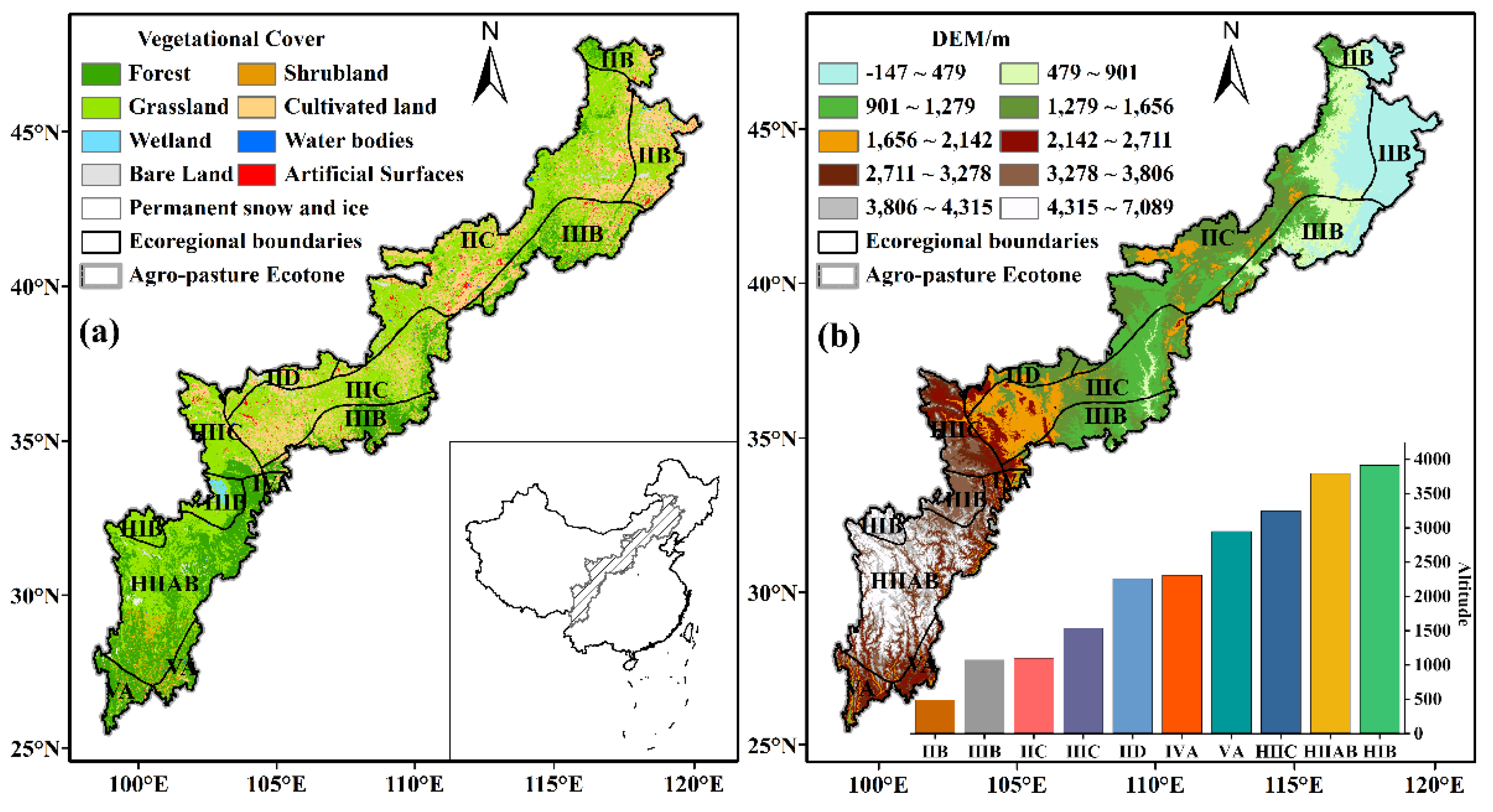
Figure 1. Distribution of the vegetation (a) and its topographic features (b) in the study area.
Remotesensing 14 05417 g001
Figure 2. Methodology for extracting the SOS and EOS from the EVI seasonal curves.
Remotesensing 14 05417 g002
Figure 3. Spatial distribution of the multi-year mean values of the vegetation phenological periods in the agro-pasture ecotone. (ac) indicate the mean changes of the SOS (a), EOS (b), and LOS (c) between 2000 and 2020, respectively. The histogram in the lower right corner indicates the percentage of the different color bands in the total; (df) Box plots of the mean SOS (d), EOS (e), and LOS (f) for the different eco-geographic regions of the study area over 21 years, respectively.
Remotesensing 14 05417 g003
Figure 4. Characteristics of the vegetation phenology with altitude change. (ac) indicate the average changes in the SOS (a), EOS (b), and LOS (c) at different altitudes, from 2000 to 2020, respectively.
Remotesensing 14 05417 g004
Figure 5. The interannual variation of the vegetation phenology in the agro-pasture ecotone. (ac) Spatial distribution of the interannual variation trends of the SOS, EOS, and LOS, between 2000 and 2020, respectively; (df) are the significances of the SOS (d), EOS (e), and LOS (f) obtained from the MK test for a period of 21 years, respectively.
Remotesensing 14 05417 g005
Figure 6. Spatial patterns of the vegetation phenological change stability in the agro-pasture ecotone. (ac) denote spatial patterns of the SOS (a), EOS (b), and LOS (c) stability, from 2000 to 2020, respectively.
Remotesensing 14 05417 g006
Figure 7. Graded ratios of the positive/negative correlation coefficients of the SOS and precipitation/temperature.
Remotesensing 14 05417 g007
Figure 8. Spatial distribution of the correlations of the SOS with precipitation (a) and temperature (b) in the month with the greatest influence on it; The inset at the bottom right of each figure shows the pixels with a significance. (c,d) indicate the proportion of correlations between the SOS and the precipitation (c) and temperature (d) of the month with the greatest influence on it for different eco-geographic regions, respectively.
Remotesensing 14 05417 g008
Figure 9. Graded ratios of the positive/negative correlation coefficients between the EOS and precipitation/temperature.
Remotesensing 14 05417 g009
Figure 10. Spatial distribution of the correlations of the EOS with precipitation (a) and temperature (b) for the month with the greatest influence on them; The inset at the bottom right of each figure shows the pixels with a significance. (c,d) indicate the proportion of correlations between the EOS and the precipitation (c) and temperature (d) of the month with the greatest influence on it for different eco-geographic regions, respectively.
Remotesensing 14 05417 g010
Table 1. Eco-geographical regional systems in the agro-pasture ecotone.
Temperature Areas (Abbreviations *)Arid and Humid Areas (Abbreviations *)Abbreviations *
Plateau temperate area (HII)Humid and semi-humid area (A/B)HIIAB
Semi-arid area (C)HIIC
Plateau sub-frigid area (HI)Semi-humid area (B)HIB
Warm temperate area (III)Semi-humid area (B)IIIB
Semi-arid area (C)IIIC
Mid-temperate area (II)Semi-humid area (B)IIB
Semi-arid area (C)IIC
Arid area (D)IID
North subtropical area (IV)Humid area (A)IVA
Mid-subtropical area (V)Humid area (A)VA
* All of the eco-geographic regions mentioned below are referred to by their abbreviations and are not repeated.
Table 2. Mann–Kendall test trend categories.
βZTrend Features
β > 0Z > 1.96Significant delayed
Z ≤ 1.96No significant delayed
β ≤ 0Z ≤ 1.96No significant earlier
Z > 1.96Significant earlier
Publisher’s Note: MDPI stays neutral with regard to jurisdictional claims in published maps and institutional affiliations.