Article

Are Climate-Dependent Impacts of Soil Constraints on Crop Growth Evident in Remote-Sensing Data?

School of Agriculture and Food Science, The University of Queensland, St. Lucia, QLD 4072, Australia
*
Author to whom correspondence should be addressed.
Remote Sens. 2022, 14(21), 5401; https://doi.org/10.3390/rs14215401
Submission received: 11 August 2022 / Revised: 12 October 2022 / Accepted: 25 October 2022 / Published: 28 October 2022

Abstract

:
Soil constraints limit plant growth and grain yield in Australia’s grain-cropping regions, with the nature of the impact dependent on climate. In seasons with low in-crop (short for “during the crop growing season”) rainfall, soil constraints can reduce yield by limiting soil water infiltration, storage, and crop water uptake. Conversely, soil constraints can exacerbate waterlogging in seasons with high in-crop rainfall. When average in-crop rainfall is experienced, soil constraints may only have a limited impact on yields. To investigate the relationship between climate and the impact of soil constraints on crop growth, long-term time series yield information is crucial but often not available. Vegetation indices calculated from remote-sensing imagery provide a useful proxy for yield data and offer the advantages of consistent spatial coverage and long history, which are vital for assessing patterns of spatial variation that repeat over many years. This study aimed to use an index of crop growth based on the enhanced vegetation index (EVI) to assess whether and how the within-field spatial variation of crop growth differed between years with different climates (dry, moderate, and wet years, as classified based on in-crop rainfall). Five fields from the grain-growing region of eastern Australia were selected and used to assess the consistency of the spatial variation of the index for years in the same in-crop rainfall category. For four of the five fields, no evidence of patterns of climate-dependent spatial variation was found, while for the other field, there was marginal evidence of spatial variation attributable to wet years. The correlation between measured data on soil sodicity (a soil constraint that might be expected to impact crop growth most in wetter years) and average EVI was investigated for this field. The results showed a stronger negative correlation between average EVI and sodicity in wet years than in dry years, suggesting that sodicity—through its impacts on soil structure and water movement—might be a driver of the spatial variation of crop growth in wet years for this field. Our results suggest that although there may be cases when climate-dependent within-field spatial variation of crop growth is detectable through remote-sensing data (through the multi-year consistency of the within-field variation), we should not expect this to be evident for fields as a matter of course.

1. Introduction

Climate variables, particularly rainfall, are important drivers controlling the availability of water to plants, thereby influencing the resulting crop growth and productivity [1,2]. Rainfall drives the temporal variation of soil moisture, and thus, the water available for plant uptake [1,3]. During dry years, plants rely more on water stored in the soil profile from the end of the previous growing season, magnifying the importance of the plant’s access to stored water.
Another influential factor for crop growth and yield is soil constraints. Soil constraints can be defined as any soil characteristic limiting crop growth and negatively impacting agricultural production. In much of the grain-growing region of eastern Australia, the most significant constraints are those related to soil salt content, namely salinity and sodicity [1,4]. Soil salinity refers to a large concentration of soluble salts in the soil solution [5,6], while soil sodicity refers to a large concentration of sodium ions (Na+) on the soil cation exchange complex (CEC; [7]). Generally, a moderate amount of soluble salt or sodium ions may benefit plants. Still, an excess of those elements may adversely affect plant growth and degrade soil structure, which can limit soil water infiltration and storage [1,5,8,9].
Spatially, across a field, plant-available soil water is controlled by the soil’s capacity to store water [3] and the plant’s capacity to extract this water for growth. The soil structural degradation associated with sodicity can limit water infiltration and storage, while the adverse physiochemical conditions created by both sodicity and salinity can reduce plant water uptake. The impact of soil constraints on plant available water and yield is dependent on climate. In growing seasons with limited in-crop (short for “during the crop growing season”) rainfall, the plant is especially reliant on access to stored soil moisture, and the presence of constraints that restrict either the storage of soil moisture or the ability of the crop to take up soil moisture is likely to reduce yield [10]. In a particularly wet growing season with abundant rainfall, we might expect soil constraints that reduce drainage and increase the susceptibility of the soil to waterlogging (for example, soil sodicity, compaction) to be important factors driving yield variation.
On the other hand, when in-crop rainfall (ICR) is reasonably consistent and sufficient for good crop growth, we might expect a limited impact of soil constraints on yield. Thus, spatial variation in yield patterns in dry and wet years might show a stronger correlation with the spatial variation of soil constraints compared with reasonably average rainfall years. Furthermore, the different patterns of spatial yield variation (within fields) between wet and dry years might be related to the spatial variation of different soil constraints. Based on this assumption, it might be possible to detect the impact of different soil constraints from yield data collected over many growing seasons. However, the availability of long-term archives of yield monitor data is limited, thus restricting the detection of soil constraints using this approach.
A valuable surrogate for yield can be derived from remote-sensing data, which offer excellent time series and spatial information [11,12]. Although remote-sensing data will not directly measure yield, it is useful to produce vegetation indices from vegetation greenness and density [12,13,14,15,16,17,18,19,20,21]. This study assumed that vegetation indices from a series of images around peak biomass (the average of the enhanced vegetation index, EVI) would best approximate the spatial variation of yield [12,13,21]. Therefore, the average EVI for each growing season might be used to identify the differences in the spatial variation of crop yield among different climate years; as a result, when compared with soil constraints data, there might be potential to detect the different impacts of soil constraints in different climate years.
The general hypothesis in this work is that soil plays an essential role in holding water for plants to extract, especially during dry years with low ICR. Therefore, we might expect the following in these dryer years: (i) more consistent patterns of within-field spatial variation of crop growth (due to a common dominant driver of the variation); and (ii) stronger correlations between soil constraints that limit the storage and the plant extraction of soil water and the average EVI across the field (locations with high constraints would have poor growth compared with locations with low constraints). Meanwhile, for wet years, we might also expect consistent growth patterns (but perhaps different patterns to those exhibited in dry years). These patterns might reflect correlations between EVI and soil constraints causing waterlogging (e.g., sodicity or compaction). Finally, in years with average ICR, the soil’s ability to store plant available water would not be so important, and other factors (e.g., pests/diseases) might be the more important drivers of variation of crop growth across the field. In these moderate climate years, we might not see a consistent spatial variation of crop growth or such significant correlations between EVI and the constraints across the field.
In this work, we integrated spectral information from remote sensing with ICR data to predict areas within fields where yield loss due to soil constraints occurs and whether this loss occurs in wet, moderate, or dry in-crop rainfall years. We followed this up by comparing the remote sensing data with soil data to investigate whether the identified rainfall-dependent variation was associated with a particular soil constraint. Accordingly, this study aimed to analyze how the average EVI best assesses soil constraints under different rainfall conditions. The research questions in this study were:
  • How does the spatial pattern of a remote-sensing-based growth index within fields differ between years, and is it related to in-crop rainfall?
  • Does the within-field pattern of average EVI in dry and wet years correlate with the spatial variation of soil constraints expected to have the most impact in these years?

2. Materials and Methods

2.1. Study Area

The study area (Figure 1) is in Australia’s northern grain-growing region (as defined previously by the Grains Research and Development Corporation of Australia, GRDC), which covers central and southern parts of Queensland and northern parts of New South Wales. The region has a semi-arid climate, with 500–800 mm annual rainfall falling mainly during summer (Figure 2), and is dominated by winter grains cropping, especially wheat, with an average yield between 1.09 t/ha–3.36 t/ha [22]. In this study, we used data from five fields from across the region, with sizes ranging from 10 to 200 ha. These fields were selected in earlier work [9,15,22,23,24,25] during which soil sampling was conducted (see Section 2.2.3). In general, soils in Australia’s northern grain-growing region are dominated by cracking clay soils (Vertosols) [7,9,15,23,25,26,27], with smaller areas of Sodosols [28] and Chromosols [29]. Specifically, the five selected fields are dominated by Vertosols.

2.2. Datasets and Pre-Processing

2.2.1. Satellite Data

This work used 30-m pixel resolution satellite imagery from Landsat-5 Thematic Mapper (TM), Landsat-7 Enhanced Thematic Mapper Plus (ETM+), and Landsat-8 Operational Land Imager (OLI) (The United Stated Geological Survey, USGS, Reston, VA, USA) collected between 1999 and 2019 (Figure 3). Standardized surface reflectance was derived [30], and cloud shadows were masked from images using the Fmask algorithm [31]. Three bands of each satellite were used, representing the blue, red, and near-infrared (NIR) portions of the electromagnetic spectrum, to calculate the enhanced vegetation index (EVI; [32]). This index has been used in previous work [33,34] and showed a reasonable correlation with crop yields in the study region. Some images were incomplete due to partial cloud coverage or the ‘SLC-off’ issue with Landsat 7. Only images with at least 75% coverage of a field were included. For incomplete images with ≥75% coverage, gaps were filled by regression kriging, as follows. First, the image (from the same season as the incomplete image) with the highest correlation with the incomplete image was selected as the covariate (provided it covered the missing pixels). Then, a linear model was fitted to predict the missing pixels before the residuals from this linear model were kriged and added to the linear function to give the fill values. For each field, the resulting dataset consisted of a set of complete EVI rasters for multiple dates (Figure 3) within each growing season from 1999 to 2019.

2.2.2. Climate Data

Daily rainfall data on each field was extracted from the nearest cell of the 5-km gridded dataset, obtained from SILO (Scientific Information for Land Owners), a database of Australian climate data (https://www.longpaddock.qld.gov.au/silo/ (accessed on 16 July 2021)). Although other climate variables are important for crop growth, only rainfall was used in this analysis to investigate whether we might see evidence of impacts of soil constraints on crop growth depending on the in-crop rainfall, with low in-crop rainfall expected to emphasize soil constraints limiting soil water availability and uptake, and high in-crop rainfall expected to emphasize constraints linked with waterlogging.

2.2.3. Soil Constraint Data

Soil constraint data (Table 1) collected in previous work [22] were further considered in the analysis. We assumed the soil constraints were temporally stable throughout the period (1999–2019). Thus, in this analysis, we used one set of soil constraint measurements taken between April–May 2009 from eight to twelve sampled soil cores per field [22]. Each sampled core was split into eight depth intervals, and data from four of these depths are considered here: 0–10 cm, 30–50 cm, 70–90 cm, and 110–130 cm. The samples were dried at 400 °C in a forced-draught oven and ground to pass through a <2-mm sieve [9]. Three variables representing soil constraints were used in this analysis: ESP (exchangeable sodium percentage) as an indicator of soil sodicity and possible dispersion effects, and ECse (electrical conductivity of a saturated paste extract) and chloride (Cl) content as indicators of soil salinity. Chloride content and EC1:5 were determined in 1:5 soil:water suspension (with the EC1:5 used with the Cl and clay content to calculate an ECse [6]). The ESP was calculated based on the ratio of exchangeable Na to CEC, determined using 1 M NH4Cl extracting solution. The sampled profiles showed considerable variation in terms of soil constraints within fields. Based on tolerance limits of wheat to soil constraints [35], Fields 1, 2, and 5 have locations with severe salinity and sodicity from a depth of 0.7 m, Field 3 has locations with severe sodicity from 1.1 m, while Field 4 has locations with severe salinity and sodicity through the entire profile. The soil data were brought into the analysis as required, as described in Section 2.4.2. The soil data were used as confirmatory data to study further variation suggested by the analysis of remote sensing data. For instance, if the remote-sensing analysis showed evidence of a consistent pattern of spatial variation in wet years, this would indicate a soil constraint impacting most wet years, such as soil sodicity, was the main driver, and soil ESP data would be analyzed.

2.3. Initial Data Processing Methods

2.3.1. Detecting Years to Be Included in the Ensuing Analysis

This analysis included remote-sensing data from 1999 to 2019. However, it would not be appropriate to include the remote-sensing data from all years in the analysis (concerning soil constraints). For some years, a crop might not have been sown (in growing seasons with limited ICR, it is common for growers to decide not to plant crops to avoid crop failure), while for other years, the remote-sensing data might be insufficient to provide a confident spatial representation of crop growth and yield. Since we aimed to provide a means of analysis based on the remote-sensing data, we defined a series of heuristics to detect the years included in the subsequent analysis. For each field, we calculated the field-median EVI for all available dates of imagery to compile a time series of field-median EVI for each year and checked that (i) there were at least five available dates in a certain year, (ii) the maximum field median EVI in a year was greater than 0.25, (iii) the maximum field-median EVI was between mid-June until end of October (indicative of the peak biomass for a winter crop), (iv) the field-median EVI both before and after the time of the peak was at some point less than half of the maximum field-median EVI (an indication of a reasonably pronounced growth curve), and (v) the data from a growing season spanned at least a 120-day interval. In addition to these heuristics, we inspected the imagery for evidence of spatially differential management (example in Figure 4) and excluded any seasons where such evidence was found. We only used data from fields managed spatially uniformly so that spatial differences in crop growth would not be due to differential management, but rather would be predominantly due to the effects of soil spatial variability.

2.3.2. Calculating an Index to Represent the Spatial Variation of Crop Yield for Each Year

From previous research [33,34], several well-known vegetation indices, such as NDVI, RVI, EVI, and EVI2, taken from around the time of their peak demonstrated good prediction of within-field yield variation for wheat crops in eastern Australia. Therefore, this study used one of those indices, EVI, averaged over a window from 64 days before until 64 days after the date of the peak of the field-median EVI. Furthermore, we filtered this series of images by only including those for which the field-median EVI was at least 60% of the peak of the field-median EVI (to avoid including imagery with very low vegetation cover). We calculated the average from these filtered images, which we refer to from hereon as the average EVI for each year. The result of this step was, for each field, a stack of average EVI rasters (one raster for each of the included years).

2.3.3. Determining In-Crop Rainfall

The yield of grain crops grown on soils of the region is potentially limited by many factors, but water supply is the dominant factor. Due to summer-dominant rainfall, winter crops largely rely on water stored in the soil profile during previous summer–autumn fallow. Therefore, in this study, we used the period from 5 months before to 3 months after the peak EVI to represent ICR. Previous work, where detailed management data were known, used a 3-month period to represent early-season ICR [9]; this study used a longer period for ICR due to the uncertainty in season dates estimated from remote-sensing data. We note that we also tested an approach using a shorter ICR period (unpublished data), which gave similar results to those presented here. For all fields, each growing season was classified into three different classes (dry, moderate, or wet years). This classification was made to keep an equal number of years within each of the three categories to enable statistical comparisons, rather than using a fixed definition of ICR (which would lead to unequal numbers of years in the different classes). We note that we also compared fixed threshold for classifying in-crop rainfall. This is explored in the discussion.

2.4. Statistical Analysis Methods

If a soil constraint, such as soil salinity, (i) is an important cause of yield loss in a field, (ii) has the most impact on yield loss in dry years, and (iii) is itself variable within a field, then we might expect the spatial variation of soil salinity to be most strongly correlated with the spatial variation of crop growth in dry years (when the supply of water to the plants from ICR is low). Similarly, for soil constraints that might impact soil structure and water infiltration (such as soil sodicity), we might expect strong correlations in years with high rainfall, when in-crop conditions might give rise to waterlogging issues for the affected soils. In both of these cases, we might expect that in years with similar in-crop climatic conditions, the spatial variation of crop growth will be more similar than in years with different climatic conditions (i.e., maps showing the spatial variation of crop growth for two dry years should be more similar to each other than a map for a wet and a map for a dry year). We propose an analysis to investigate whether these stronger correlations are evident in remote-sensing data (the average EVI). We follow this analysis up for fields where strong correlations associated with climate are evident, by overlaying the remote-sensing (average EVI) data with soil data.

2.4.1. Assessing Relative Growth Index Consistency within a Certain Climate Year Classification

The first analysis in this work was to test whether there was evidence of distinct patterns of spatial variation for years with a specific ICR class. The assessment used an index called the relative growth index (RGI) to represent the spatial variation of crop growth within a field in a given year. To calculate the RGI, the pixels in a growing season’s average EVI map were ranked, and these pixel rankings were standardized to the range 0–100; thus, the RGI represented the ‘good’ and ‘bad’ performing parts of the field and the consistency of the RGI over multiple years could be investigated. In general, we looked for evidence that the spatial variation of RGI was more consistent for maps from years with the same climate classification than for maps with different classifications.
Suppose we have N years, indexed here by i = 1, …, N, to be included in the analysis (see Section 3.1), and that the subset iW of these years is classed as wet, the subset iM is classed as moderate years, and the subset iD is classed as dry years. The sizes of subsets iW, iM, and iD are all equal to the integer part of N/3 (meaning that all N years are not necessarily included). For the subset iW, (and after that, iM and iD, in turn) we calculate the mean and variance of the RGI and use values to calculate the p-value from a one-sample t-test assessing whether the mean RGI for the pixel is less than or greater than 50. The pixels with mean RGI < 50 and p < 0.05 are labeled as ‘consistently poor’ (relative to the field median), while the pixels with mean RGI > 50 and p < 0.05 are labeled as ‘consistently good’, with the remaining pixels labeled as ‘inconsistent/moderate’. Furthermore, we define a ‘consistency index’ (CI) as the percentage of pixels classed as either consistently poor or consistently good. This CI can range from 0, if the maps in a subset of years all showed different patterns of spatial variation, to 100, if the maps in a subset all showed identical patterns of spatial variation.
We apply a bootstrapping method to assess whether the calculated CI for a particular subset of years represents more consistent variation than we would expect ‘by chance’. This was done by selecting a random subset of years (of the same size as subsets iW, iM, and iD) from the included years and recalculating the CI. This bootstrapping procedure was repeated 1000 times to generate a distribution of the test statistic (the CI) under the null hypothesis of no increased consistency attributable to certain in-crop climate conditions. We deemed a subset of years potentially interesting—with evidence of a distinct pattern of spatial variation in the particular group of years—if the actual calculated CI was larger than the 95th percentile of the bootstrapped CI values. A corresponding p-value was calculated as the proportion of bootstrapped CI values that were larger than the real CI value, which was adjusted to account for multiple hypothesis testing (comparisons made for five fields) using the Benjamini–Hochberg correction.

2.4.2. Comparing Remote-Sensing Data with Data on Soil Constraints

When the analysis described in Section 2.4.1 suggested a particular pattern of spatial variation of crop growth associated with a particular set of climate-classified years, we followed up the analysis by comparing the remote sensing data with soil data. The remote sensing data are maps of the average EVI (Section 2.3.2), averaged over the years in the same ICR class. Thus, three different average EVI maps are used for each field, representing the variation of growth observed in wet, moderate, and dry years. The average EVI values were extracted from these maps for each pixel where soil profiles (Section 2.2.3) are located for comparison with the soil data. This comparison aimed to assess soil constraints related to crop growth (represented by the average EVI) under different in-crop climates. We did this by assessing linear regression lines between average EVI values and soil constraints data from all soil profiles in a field and compared these regressions for average EVI values under different in-crop climates.
All analyses were conducted using R 4.0.2 (R Core team, Vienna, Austria) [36].

3. Results

3.1. Cropped Years and Climate Classifications for Each Field

The simple heuristic analysis applied to detect years included in the analysis (Section 2.3.1) resulted in between 9 and 16 of the 21 considered years being included for the five fields. This gave between 3 and 5 years classified as dry, moderate, or wet (Table 2).

3.2. Concistency Analysis

Overall, from the five fields analyzed, there is no distinctive result among years classified as dry, moderate, and wet (Table 3). Based on the ICR classification, three fields (Fields 2, 4 and 5) have the largest consistency index (CI) during moderate rainfall and two fields (Fields 1 and 3) during wet years.
The bootstrapping analysis revealed that only in Field 1 in wet years did the CI exceed the 95th percentile of bootstrap-sampled CI values. Furthermore, when multiple hypothesis testing was accounted for, only Field 1 in wet years showed a larger than expected CI value (marginally significant at p < 0.1). This suggests that for Field 1 in wet years, there might be something driving spatial variation of crop growth that impacts differently in moderate or dry years.
The distribution of the consistent pixels within each of the five fields is presented using color coding, where red and green pixels are the areas with consistently low (mean RGI < 50) and high (mean RGI > 50) ranks among years in the same climate class (Figure 5). For Field 1, the field with a greater than expected CI in wet years, the westerly and easterly ends of the field showed consistently poor growth in wet years, while the central part of the field showed consistently good growth in wet years, which was not evident in the moderate or low rainfall years.

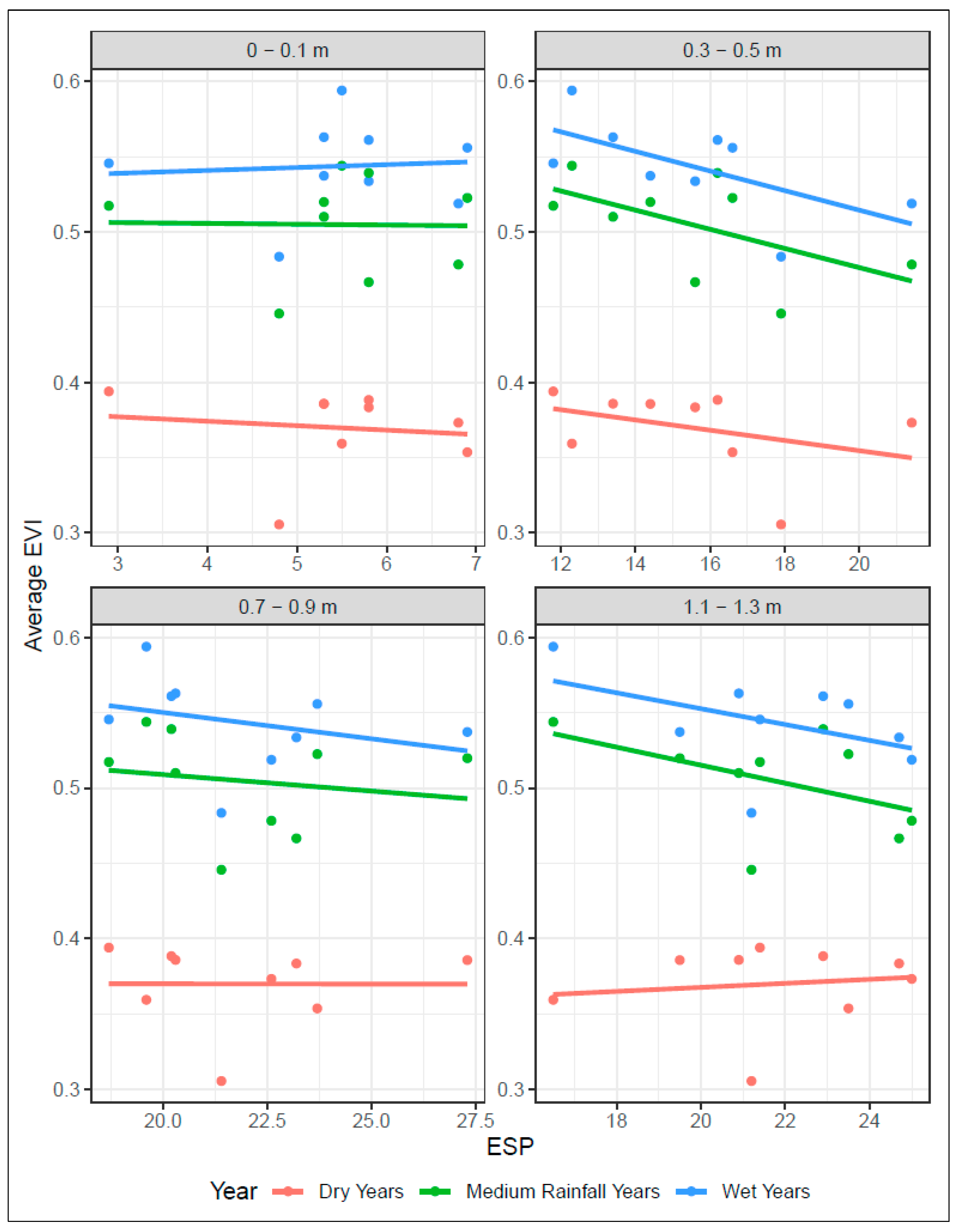
3.3. Analysis with Soil Constraint Data

Since the remote sensing data analysis indicated that Field 1 exhibited a significantly higher than expected consistency of variation in wet years (albeit marginally significant at p < 0.1), soil data from the field were used to investigate this variation. Further, the soil ESP data were used for this analysis because soil sodicity might be expected to impact crop growth most in wet years.
When data for soil sodicity (indicated by high values of the ESP) for different soil depths (0–0.1 m, 0.3–0.5 m, 0.7–0.9 m, and 1.1–1.3 m) and the average EVI in dry moderate and wet years are considered (Figure 6), only the subsoil data (>0.3 m) showed a relationship, where the higher the ESP, the lower the average EVI. This agrees with what might be expected, indicating that the higher the sodicity, the lower the yield. For the topsoil, there was no such evident pattern, indicating that topsoil sodicity is not an important driver of yield variation in this field. When comparing the average EVI between different climate years, wet years had the highest values, followed by moderate and dry climate years (as would be expected). Amongst the scatter around the fitted regression lines, the data from one soil profile consistently showed an EVI below the fitted line (for all rainfall years and all soil depths). This outlier comes from the soil profile with the lowest EVI in each rainfall year. The possible reason for this is that the location of the soil profile, which is close to the field boundary, could negatively influence crop growth [37].
Furthermore, when comparing the slope of a linear regression line (Figure 6) between average EVI and ESP for wet (blue line), moderate (green line), and dry years (red line), the wet and moderate year regressions have steeper (negative) slopes than dry years (apart from in the topsoil). However, while these relationships agree with what might be expected of sodic soils (stronger effects of sodicity in wet years [1,38,39,40]), the evidence in the data for this is limited.

4. Discussion

Our research tested the hypothesis that soil constraints would drive within-field yield variation more in dry and wet rather than moderate rainfall. This would be evident in remote-sensing data through more consistent spatial variation of growth in these years. Previous studies found a more pronounced negative impact of soil salinity leading to yield reduction during dry years [9,25,41,42]. In our analysis, the remote-sensing data did not show evidence of within-field spatial variation associated with dry years. However, for one of the five fields (Field 1), the remote-sensing data did show some evidence (p < 0.1) of more consistent spatial variation associated with climate in years with high ICR. One possible explanation for this is the occurrence of extreme rainfall events, which may have induced waterlogging where soils were sodic and had poor internal drainage [1,38,39,40]. Indeed, further analysis of the soil data for this field demonstrated that subsoil ESP was negatively related to crop growth (represented by the average EVI), most strongly in wet and moderate rainfall years.
For four of the five fields, no climate-dependent spatial variation in crop growth was evident in the remote-sensing data. One possible reason is that the classification of years based on ICR over the entire season is a simplification that does not necessarily indicate the assumed effects of soil constraints. Therefore, more in-depth climate analysis to indicate years with potential problems might be considered for future studies, for instance, using crop simulation models such as WOFOST (World Food Studies; [43]) or APSIM (Agricultural Production Systems Simulator; [27,42,44]), which has been widely used to model yield under constrained soils and to simulate the effects of salinity and sodicity on crop growth. This simulation model-based approach might provide a better indication of the years when crop growth is most likely to be affected by soil constraints, and therefore the years when we might expect more consistent patterns of within-field spatial variation of growth that have the strongest correlation with those soil constraints.
Another factor that might have impacted results is the spatial resolution of the remote sensing data obtained from the Landsat series of satellites [45]. The Landsat satellites were used due to the need for a long data history, and thus enough years falling into each rainfall class. Other freely available imagery, such as that from the more recently launched Sentinel satellites, offers a more refined spatial resolution (10-m compared with 30-m), although this data is not available for as long. Some form of fusion of the data for the two sources might improve future work.
For this analysis, for a given field, we forced equal numbers of years in the three climate classes (wet, moderate, and dry years) by defining the categories based on the quantiles of ICR. An alternative would be to consider fixed definitions of wet, moderate, and dry years. This would lead to different numbers of years in the different classes (unbalanced data), although this alternative would have benefits regarding relevance to these fixed definitions of climate. We tested the impact of this on results by applying absolute thresholds of ICR to categorize years; results from this alternative analysis (see Appendix A and Appendix B, Table A1 and Figure A1) were similar, with only marginally significant climate-dependent variation associated with wet years in Field 1. For our analysis, the fixed number of years in each class meant between three and five years in each climate year classification for the five fields. This small number of years in each classification limits the analysis because the influence of individual years on analysis can be strong. For instance, if there were just three years in each class and one of three dry years in the analysis had some other problem driving variation that year (e.g., crop disease in part of the field), then the consistency of the three maps could be impacted substantially, giving a much smaller consistency index. This limitation could be prevented if the analysis covered more years.
Besides using rainfall to classify climate years, we also tried to group climate years based on vapour pressure deficit (VPD), which is the difference between actual and saturated vapour pressure [46]. The VPD, which is negatively correlated with rainfall, could also act as an alternative climate indicator to rainfall that indirectly influences the temporal variation of soil moisture. Overall, results from analysis based on VPD classification (Table A2) were similar to those based on rainfall classification, with only Field 1 in wet years (low VPD) exceeding the 95th percentile of bootstrap-sampled CI values (i.e., showing some evidence of a pattern of climate-dependent variation). This supports the results from the rainfall analysis.
Although our analysis has revealed no compelling evidence that climate-dependent impacts of soil constraints would be routinely revealed in remote-sensing data, there is still a possibility to expand the simple rainfall-based analysis with the support of other climate variables and/or models. In the future, the concept could be useful for underpinning software such as ConstraintID (https://constraintid.net.au/ (accessed on 16 July 2021)) [47,48]. This software enables growers to overlay remote-sensing data with soil data, providing them with useful information to diagnose reasons for spatial variation of crop yields within fields. If future analyses revealed more compelling evidence of climate-dependent patterns of growth within fields (associated with climate-dependent impacts of soil constraints)—evidence of such effects occurring in multiple fields—this could be readily incorporated in the software.
In summary, we have investigated an approach to identify climate-dependent within-field spatial variation in crop growth based on remote sensing and rainfall data. When this analysis suggested some climate-dependent spatial variation in crop growth (EVI) might be present for a field, we followed up by aligning the remote-sensing data with relevant soil constraints data (for a soil constraint that might be expected to impact in the identified climate, such as soil sodicity in wet years) to check whether spatial variation in the soil constraint was associated with the variation in EVI. We assessed how far remote sensing, supported by some climate data such as ICR, can elicit climate-dependent spatial variation of crop growth that could be confirmed to be driven by soil constraints. However, our results suggested that soil constraint effects might only be apparent in certain locations.

5. Conclusions

In this work, we investigated the potential of remote-sensing imagery to diagnose the impacts of soil constraints in different climate years. We initially assessed the consistency of growth patterns over the years classified by rainfall. The results showed that from the five fields investigated, only one field showed a marginally significant consistency pattern, showing a distinct pattern of spatial variation associated with wet (high ICR) years. The follow-up analysis for this field, aligning the remote-sensing data with soil data, determined whether the variation might be associated with soil sodicity, which can impact crop growth in particular when abundant rainfall leads to issues with soil structure, poor water infiltration, and waterlogging. The field’s results indicated that higher subsoil sodicity was associated with poorer crop growth, particularly during the wet years. Our results suggest that although there may be cases when the climate-dependent within-field spatial variation of crop growth is detectable through remote-sensing data, we should not expect this to be evident. Further investigation of alternative analyses might shed more light on the issue in future.

Author Contributions

Conceptualization: F.U., T.G.O., Y.P.D. and N.W.M.; Methodology: F.U. and T.G.O.; Analysis and result interpretation: F.U. and T.G.O.; Writing—original draft preparation: F.U.; Writing—review and editing: T.G.O., Y.P.D. and N.W.M. All authors have read and agreed to the published version of the manuscript.

Funding

This work was funded by the Grains Research and Development Corporation (GRDC) of Australia under project number UOQ1803-003RTX.

Data Availability Statement

The datasets generated during and/or analysed during the current study are available from the corresponding author on reasonable request.

Acknowledgments

Landsat imagery is provided by the United States Geological Survey, and the support and resources provided by the Queensland Remote Sensing Centre, Department of Environment and Science, and the help of Matt Pringle, is gratefully acknowledged. The authors also thank for helpful discussions from Scott Chapman.

Conflicts of Interest

The authors declare no conflict of interest.

Appendix A

Table A1. Consistency index in different climate years when ICR group classified based on thresholds (dry years < 160 mm, moderate years = 160–240 mm, wet years > 240 mm). A number inside brackets indicate the number of years within each group. Bold values indicate marginally significant adjusted p values (p < 0.1). NA values are indicating statistically not enough data for the analysis.
FieldsICRICR Bootstrap 95% Percentile
DryModerateWetDryModerateWet
Field 122.73 (5)NA (2)53.03 (9)37.12NA43.18
Field 223.94 (4)27.13 (3)46.28 (9)40.4335.6452.13
Field 375.26 (3)73.84 (5)NA (1)82.2989.74NA
Field 4NA (2)7.11 (3)47.25 (9)23.6538.3954.98
Field 545.17 (8)NA (1)NA (1)47.06NANA

Appendix B

Figure A1. The relationship between average EVI (climate years were grouped by pre-defined ICR thresholds) and soil ESP for four soil depths at Field 1 for dry and wet years.
Remotesensing 14 05401 g0a1

Appendix C

Table A2. Consistency index in different climate years based on in-crop vapor pressure deficit (ICVPD). Bold values indicate marginally significant adjusted p values (p < 0.1).
FieldsDryModerateWetBootstrap 95% Percentile
Field 120.8318.9440.9139.03
Field 234.5824.4723.4043.62
Field 375.2647.4971.8382.29
Field 434.0920.1017.0741.09
Field 527.7113.9212.5736.64

References

  1. Weil, R.R.; Brady, N.C. The Nature and Properties of Soils, Global Edition, 15th ed.; Pearson Education Limited: London, UK, 2017. [Google Scholar]
  2. Yuan, W.; Zheng, Y.; Piao, S.; Ciais, P.; Lombardozzi, D.; Wang, Y.; Ryu, Y.; Chen, G.; Dong, W.; Hu, Z.; et al. Increased atmospheric vapor pressure deficit reduces global vegetation growth. Sci. Adv. 2019, 5, 1–13. [Google Scholar] [CrossRef] [PubMed] [Green Version]
  3. Tang, C.; Asseng, S.; Diatloff, E.; Rengel, Z. Modelling yield losses of aluminium-resistant and aluminium-sensitive wheat due to subsurface soil acidity: Effects of rainfall, liming and nitrogen application. Plant Soil 2003, 254, 349–360. [Google Scholar] [CrossRef]
  4. SalCon. Salinity Management Handbook; Queensland Departement of Natural Resources and Mines, Indooroopilly, Qld: Brisbane, Australia, 1997. [Google Scholar]
  5. Page, K.L.; Dalal, R.C.; Wehr, J.B.; Dang, Y.P.; Kopittke, P.M.; Kirchhof, G.; Fujinuma, R.; Menzies, N.W. Management of the major chemical soil constraints affecting yields in the grain growing region of Queensland and New South Wales, Australia—A review. Soil Res. 2018, 56, 765. [Google Scholar] [CrossRef]
  6. Shaw, R.J. Soil Salinity—Electrical Conductivity and Chloride. In Soil Analysis: An Interpretation Manual; Peverill, K.I., Sparrow, L.A., Reuter, D.J., Eds.; CSIRO Publishing: Collingwood, Australia, 1999. [Google Scholar]
  7. Dang, Y.P.; Dalal, R.C.; Routley, R.; Schwenke, G.D.; Daniells, I.G. Subsoil constraints to grain production in the cropping soils of the north-eastern region of Australia: An overview. Aust. J. Exp. Agric. 2006, 46, 19–35. [Google Scholar] [CrossRef] [Green Version]
  8. Sheldon, A.R.; Dalal, R.C.; Kirchhof, G.; Kopittke, P.M.; Menzies, N.W. The effect of salinity on plant-available water. Plant Soil 2017, 418, 477–491. [Google Scholar] [CrossRef]
  9. Dang, Y.P.; Dalal, R.C.; Buck, S.R.; Harms, B.; Kelly, R.; Hochman, Z.; Schwenke, G.D.; Biggs, A.J.W.; Ferguson, N.J.; Norrish, S. Diagnosis, extent, impacts, and management of subsoil constraints in the northern grains cropping region of Australia. Aust. J. Soil Res. 2010, 48, 105–119. [Google Scholar] [CrossRef]
  10. Rodriguez, D.; Nuttall, J.; Sadras, V.O.; Rees, H.V.; Armstrong, R. Impact of subsoil constraints on wheat yield and gross margin on fine-textured soils of the southern Victorian Mallee. Aust. J. Agric. Res. 2006, 57, 355–365. [Google Scholar] [CrossRef] [Green Version]
  11. Cai, Y.; Guan, K.; Peng, J.; Wang, S.; Seifert, C.; Wardlow, B.; Li, Z. A high-performance and in-season classification system of field-level crop types using time-series Landsat data and a machine learning approach. Remote Sens. Environ. 2018, 210, 35–47. [Google Scholar] [CrossRef]
  12. Semeraro, T.; Mastroleo, G.; Pomes, A.; Luvisi, A.; Gissi, E.; Aretano, R. Modelling fuzzy combination of remote sensing vegetation index for durum wheat crop analysis. Comput. Electron. Agric. 2018, 156, 684–692. [Google Scholar] [CrossRef]
  13. Bai, T.; Zhang, N.; Mercatoris, B.; Chen, Y. Jujube yield prediction method combining Landsat 8 vegetation index and the phenological length. Comput. Electron. Agric. 2019, 162, 1011–1027. [Google Scholar] [CrossRef]
  14. Cai, Y.; Guan, K.; Lobell, D.; Potgieter, A.B.; Wang, S.; Peng, J.; Xu, T.; Asseng, S.; Zhang, Y.; You, L.; et al. Integrating satellite and climate data to predict wheat yield in Australia using machine learning approaches. Agric. For. Meteorol. 2019, 274, 144–459. [Google Scholar] [CrossRef]
  15. Dang, Y.P.; Moody, P.W. Quantifying the costs of soil constraints to Australian agriculture: A case study of wheat in north-eastern Australia. Soil Res. 2016, 54, 700–707. [Google Scholar] [CrossRef]
  16. Goodwin, A.W.; Lindsey, L.E.; Harrison, S.K.; Paul, P.A. Estimating wheat yield with normalized difference vegetation index and fractional green canopy cover. Crop. Forage Turfgrass Manag. 2018, 4, 1–6. [Google Scholar] [CrossRef] [Green Version]
  17. Kobayashi, N.; Tani, H.; Wang, X.; Sonobe, R. Crop classification using spectral indices derived from Sentinel-2A imagery. J. Inf. Telecommun. 2020, 4, 67–90. [Google Scholar] [CrossRef]
  18. Lai, Y.R.; Pringle, M.J.; Kopittke, P.M.; Menzies, N.W.; Orton, T.G.; Dang, Y.P. An empirical model for prediction of wheat yield, using time-integrated Landsat NDVI. Int. J. Appl. Earth Obs. Geoinf. 2018, 72, 99–108. [Google Scholar] [CrossRef]
  19. Orton, T.G.; Mallawaarachchi, T.; Pringle, M.J.; Menzies, N.W.; Dalal, R.C.; Kopittke, P.M.; Searle, R.; Hochman, Z.; Dang, Y.P. Quantifying the economic impact of soil constraints on Australian agriculture: A case-study of wheat. L. Degrad. Dev. 2018, 29, 3866–3875. [Google Scholar] [CrossRef]
  20. Rouse, J.W.; Hass, R.H.; Schell, J.A.; Deering, D.W. Monitoring vegetation systems in the great plains with ERTS. Third Earth Resour. Technol. Satell. Symp. 1973, 1, 309–317. [Google Scholar]
  21. Zhao, Y.; Potgieter, A.B.; Zhang, M.; Wu, B.; Hammer, G.L. Predicting wheat yield at the field scale by combining high-resolution Sentinel-2 satellite imagery and crop modelling. Remote Sens. 2020, 12, 1024. [Google Scholar] [CrossRef] [Green Version]
  22. Dang, Y.P.; Dalal, R.C.; Christopher, J.; Apan, A.A.; Pringle, M.J.; Bailey, K.; Biggs, A.J.W. Managing Subsoil Constraints Advanced Techniques for Managing Subsoil Constraints Project Results Book; Grains Research & Development Corporation: Canberra, Australia, 2010. [Google Scholar]
  23. Dang, Y.P.; Pringle, M.J.; Schmidt, M.; Dalal, R.C.; Apan, A. Identifying the spatial variability of soil constraints using multi-year remote sensing. Field Crop. Res. 2011, 123, 248–258. [Google Scholar] [CrossRef]
  24. Dang, Y.P.; Dalal, R.C.; Pringle, M.J.; Biggs, A.J.W.; Darr, S.; Sauer, B.; Moss, J.; Payne, J.; Orange, D. Electromagnetic induction sensing of soil identifies constraints to the crop yields of north-eastern Australia. Soil Res. 2011, 49, 559–571. [Google Scholar] [CrossRef]
  25. Dang, Y.P.; Dalal, R.C.; Mayer, D.G.; McDonald, M.; Routley, R.; Schwenke, G.D.; Buck, S.R.; Daniells, I.G.; Singh, D.K.; Manning, W.; et al. High subsoil chloride concentrations reduce soil water extraction and crop yield on Vertosols in north-eastern Australia. Aust. J. Agric. Res. 2008, 59, 321. [Google Scholar] [CrossRef]
  26. Page, K.L.; Dalal, R.C.; Menzies, N.W.; Strong, W.M. Nitrification in a Vertisol subsoil and its relationship to the accumation of ammonium-nitrogen at depth. Aust. J. Soil Res. 2002, 40, 727–735. [Google Scholar] [CrossRef]
  27. Hochman, Z.; Probert, M.; Dalgliesh, N.P. Developing testable hypotheses on the impacts of sub-soil constraints on crops and croplands using the cropping systems simulator APSIM. In Proceedings of the 4th International Crop Science Congress, Brisbane, Australia, 26 September 2004. [Google Scholar]
  28. Dang, Y.P.; Routley, R.; McDonald, M.; Dalal, R.C.; Alsemgeest, V.; Orange, D. Effects of chemical subsoil constraints on lower limit of plant available water for crops grown in southwest Queensland. In Proceedings of the 4th International Crop Science Congress, Brisbane, Australia, 26 September 2004. [Google Scholar]
  29. Thomas, G.A.; Gibson, G.; Nielsen, R.G.H.; Martin, W.D.; Radford, B.J. Effects of tillage, stubble, gypsum, and nitrogen fertiliser on cereal cropping on a red-brown earth in south-west Queensland. Aust. J. Exp. Agric. 1995, 35, 997–1008. [Google Scholar] [CrossRef]
  30. Flood, N.; Danaher, T.; Gill, T.; Gillingham, S. An operational scheme for deriving standardised surface reflectance from landsat TM/ETM+ and SPOT HRG imagery for eastern Australia. Remote Sens. 2013, 5, 83–109. [Google Scholar] [CrossRef] [Green Version]
  31. Zhu, Z.; Wang, S.; Woodcock, C.E. Improvement and expansion of the Fmask algorithm: Cloud, cloud shadow, and snow detection for Landsats 4-7, 8, and Sentinel 2 images. Remote Sens. Environ. 2015, 159, 269–277. [Google Scholar] [CrossRef]
  32. Huete, A.; Didan, K.; Miura, T.; Rodriguez, E.; Gao, X.; Ferreira, L. Overview of the radiometric and biophysical performance of the MODIS vegetation indices. Remote Sens. Environ. 2002, 83, 195–213. [Google Scholar] [CrossRef]
  33. Ulfa, F.; Orton, T.G.; Dang, Y.P.; Menzies, N.W. Developing and Testing Remote-Sensing Indices to Represent within-Field Variation of Wheat Yields: Assessment of the Variation Explained by Simple Models. Agronomy 2022, 12, 384. [Google Scholar] [CrossRef]
  34. Ulfa, F.; Orton, T.G.; Dang, Y.P.; Menzies, N.W. A comparison of remote-sensing vegetation indices for assessing within-field variation of wheat yield. In Proceedings of the 20th Agronomy Conference. Toowoomba, Queensland, Australia, 18–22 September 2002. [Google Scholar]
  35. Page, K.L.; Dang, Y.P.; Martinez, C.; Dalal, R.C.; Wehr, J.B.; Kopittke, P.M.; Orton, T.G.; Menzies, N.W. Review of crop-specific tolerance limits to acidity, salinity, and sodicity for seventeen cereal, pulse, and oilseed crops common to rainfed subtropical cropping systems. L. Degrad. Dev. 2021, 32, 2459–2480. [Google Scholar] [CrossRef]
  36. R Core team. R: A Language and Environment for Statistical Computing; R Foundation for Statistical Computing: Vienna, Austria, 2020. [Google Scholar]
  37. Robinson, S.V.J.; Nguyen, L.H.; Galpern, P. Livin’ on the edge: Precision yield data shows evidence of ecosystem services from field boundaries. Agric. Ecosyst. Environ. 2022, 333, 107956. [Google Scholar] [CrossRef]
  38. Armstrong, R.D.; Eagle, C.; Flood, R. Improving grain yields on a sodic clay soil in a temperate, medium-rainfall cropping environment. Crop Pasture Sci. 2015, 66, 492–505. [Google Scholar] [CrossRef]
  39. Gill, J.S.; Sale, P.W.G.; Tang, C. Amelioration of dense sodic subsoil using organic amendments increases wheat yield more than using gypsum in a high rainfall zone of southern Australia. Field Crop. Res. 2008, 107, 265–275. [Google Scholar] [CrossRef]
  40. Gardner, W.K.; Fawcett, R.G.; Steed, G.R.; Pratley, J.E.; Whitfield, D.; van Rees, H. Crop Production on Duplex Soils: An Introduction. Aust. J. Exp. Agric. 1992, 32, 797–800. [Google Scholar] [CrossRef]
  41. Hussain, N.; Mujeeb, F.; Sarwar, G.; Hassan, G.; Ullah, M.K. Soil salinity/sodicity and ground water quality changes in relation to rainfall and reclamation activities. In Proceedings of the International Workshop on Conjunctive Water Management for Sustainable Irrigated Agriculture in South Asia, Lahore, Pakistan, 16–17 April 2002. [Google Scholar]
  42. Sadras, V.; Baldock, J.; Roget, D.; Rodriguez, D. Measuring and modelling yield and water budget components of wheat crops in coarse-textured soils with chemical constraints. Field Crop. Res. 2003, 84, 241–260. [Google Scholar] [CrossRef]
  43. Kotlar, A.M.; Everaer, B.; Blanchy, G.; Huits, D.; Garré, S. The potential of adaptive drainage to control salinization in Polder context. In Proceedings of the EGU General Assembly, Vienna, Austria, 23–27 May 2022. [Google Scholar]
  44. Hochman, Z.; Dang, Y.P.; Schwenke, G.D.; Dalgliesh, N.P.; Routley, R.; McDonald, M.; Daniells, I.G.; Manning, W.; Poulton, P.L. Simulating the effects of saline and sodic subsoils on wheat crops growing on Vertosols. Aust. J. Agric. Res. 2007, 58, 802–810. [Google Scholar] [CrossRef]
  45. Reddy, G.P.O. Geospatial Technologies in Land Resources Mapping, Monitoring, and Management: An Overview; Springer Nature: Cham, Switzerland, 2018. [Google Scholar]
  46. Rawson, H.M.; Begg, J.E.; Woodward, R.G. The effect of atmospheric humidity on photosynthesis, transpiration and water use efficiency of leaves of several plant species. Planta 1977, 134, 5–10. [Google Scholar] [CrossRef] [PubMed]
  47. Orton, T.G.; Mcclymont, D.; Page, K.L.; Menzies, N.W.; Dang, Y.P. ConstraintID: An online software tool to assist grain growers in Australia identify areas affected by soil constraints. Comput. Electron. Agric. 2022, 202, 107422. [Google Scholar] [CrossRef]
  48. Dang, Y.P.; Orton, T.G.; Mcclymont, D.; Menzies, N.W. ConstraintID: A free web-based tool for spatial diagnosis of soil constraints. In Proceeding of the 20th Agronomy Conference, Toowoomba, Queensland, Australia, 18–22 September 2022. [Google Scholar]
Figure 1. The study area in Australia’s northern grain-growing region, and the five fields considered in this analysis.
Remotesensing 14 05401 g001
Figure 2. Average monthly rainfall, in mm. Fields 1 and 2 are close to each other and have the same climate data.
Remotesensing 14 05401 g002
Figure 3. Number of images by year in the five fields.
Remotesensing 14 05401 g003
Figure 4. The average EVI from six years for Field 4 to illustrate (a) years where split management was identified based on the imagery and (b) where no such split management was identified.
Remotesensing 14 05401 g004
Figure 5. Consistency maps for all five fields in low, moderate and high ICR years. Green = consistently high, red = consistently low, yellow = inconsistent/moderate.
Remotesensing 14 05401 g005
Figure 6. The relationship between average EVI and soil ESP for four soil depths at Field 1 for dry, moderate, and wet years.
Remotesensing 14 05401 g006
Table 1. Mean values (min, max) of soil properties for each of the five fields in the study area.
Soil DepthClECseESPpHClay
Field 1
0.0521 (20, 25)0.60 (0.42, 0.79)5.5 (2.9, 6.9)7.6 (6.9, 8.4)41 (27, 48)
0.40191 (36, 512)2.19 (1.08, 4.57)15.5 (11.8, 21.4)8.9 (8.5, 9.1)49 (42, 56)
0.801159 (800, 1940)10.76 (6.31, 18.76)21.9 (18.7, 27.3)7.7 (5.4, 8.7)52 (44, 61)
1.201861 (1400, 2390)12.44 (9.2, 21.58)21.7 (16.5, 25)6.4 (4.5, 8.5)53 (47, 60)
Field 2
0.0522 (20, 36)0.59 (0.41, 1.03)3.5 (1.6, 5)7.2 (6.1, 8.4)32 (24, 42)
0.40137 (45, 307)1.97 (1.28, 3.18)13.1 (9.9, 17.3)8.8 (8.7, 8.9)42 (37, 50)
0.80827 (479, 1660)8.13 (4.8, 18.01)22.4 (19.1, 27.4)7.6 (5.3, 9)43 (38, 52)
1.201329 (940, 2060)9.28 (6.62, 12.16)23.7 (20.3, 28.5)6.1 (4.4, 8.4)47 (37, 55)
Field 3
0.0520 (20, 20)0.44 (0.31, 0.59)1.1 (0.4, 1.9)8.1 (6.5, 8.7)49 (38, 60)
0.4020 (20, 24)0.52 (0.24, 0.76)4.8 (0.6, 11)8.7 (7.4, 9)51 (39, 62)
0.8068 (20, 138)1.19 (0.43, 1.96)10.3 (0.4, 17.4)9.1 (8.5, 9.4)50 (22, 63)
1.20339 (20, 763)2.81 (0.58, 5.1)13.9 (0.2, 20.6)8.8 (8.1, 9.4)53 (28, 67)
Field 4
0.05419 (20, 1470)2.71 (0.4, 7.92)5.8 (2.3, 11.2)7.7 (7.2, 8.8)60 (56, 69)
0.401158 (47, 2170)10.43 (1.32, 21.78)16.1 (5, 27.9)8.2 (7.8, 8.9)61 (55, 68)
0.801866 (436, 3270)20.5 (13.06, 26.38)22.1 (15.3, 28.4)7.8 (7.7, 7.9)61 (55, 68)
1.202592 (1080, 4490)20.05 (15.46, 23.56)25.2 (17.7, 32)8 (7.7, 8.2)67 (59, 75)
Field 5
0.0552 (20, 132)0.72 (0.34, 1.32)8.2 (3, 12)7.6 (7.1, 8)37 (27, 49)
0.40324 (52, 668)2.6 (0.93, 4.43)20.4 (15, 28.1)8.6 (7.2, 9)54 (42, 60)
0.80831 (564, 1220)5.67 (3.77, 8.68)29 (20.1, 45.8)6.7 (4.7, 8.5)54 (40, 63)
1.20997 (781, 1320)6.35 (4.78, 8.12)36.5 (25.1, 48.7)4.8 (4.4, 5.2)55 (44, 62)
Table 2. In-crop rainfall (ICR) classification.
FieldsDry YearsModerate YearsWet Years
12002, 2004, 2006, 2009, 20182001, 2005, 2011, 2015, 20172003, 2007, 2008, 2010, 2016
22002, 2004, 2006, 2009, 20191999, 2001, 2003, 2005, 20172007, 2008, 2010, 2011, 2016
32002, 2013, 20172000, 2003, 20061999, 2007, 2012
42006, 2009, 2012, 20132003, 2005, 2014, 20152004, 2011, 2016, 2017
52002, 2005, 20172003, 2007, 20141999, 2004, 2010
Table 3. Consistency index in different climate years based on in-crop rainfall (ICR). Bold values indicate marginally significant adjusted p values (p < 0.1).
FieldsDryModerateWetBootstrap 95% Percentile
Field 122.7316.6744.3136.00
Field 223.4042.5536.1744.18
Field 375.2647.6975.4682.29
Field 416.4322.5922.1637.76
Field 512.4327.0312.5734.58
Publisher’s Note: MDPI stays neutral with regard to jurisdictional claims in published maps and institutional affiliations.

