Article

MiPo: How to Detect Trajectory Outliers with Tabular Outlier Detectors

1
School of Marine Science and Technology, Northwestern Polytechnical University, Xi’an 710072, China
2
School of Computing, University of Eastern Finland, FI-80101 Joensuu, Finland
*
Author to whom correspondence should be addressed.
These authors contributed equally to this work.
Remote Sens. 2022, 14(21), 5394; https://doi.org/10.3390/rs14215394
Submission received: 21 September 2022 / Revised: 10 October 2022 / Accepted: 11 October 2022 / Published: 27 October 2022

Abstract

:
Trajectory outlier detection is one of the fundamental data mining techniques used to analyze the trajectory data of the Global Positioning System. A comprehensive literature review of trajectory outlier detectors published between 2000 and 2022 led to a conclusion that conventional trajectory outlier detectors suffered from drawbacks, either due to the detectors themselves or the pre-processing methods for the variable-length trajectory inputs utilized by detectors. To address these issues, we proposed a feature extraction method called middle polar coordinates (MiPo). MiPo extracted tabular features from trajectory data prior to the application of conventional outlier detectors to detect trajectory outliers. By representing variable-length trajectory data as fixed-length tabular data, MiPo granted tabular outlier detectors the ability to detect trajectory outliers, which was previously impossible. Experiments with real-world datasets showed that MiPo outperformed all baseline methods with 0.99 AUC on average; however, it only required approximately 10% of the computing time of the existing industrial best. MiPo exhibited linear time and space complexity. The features extracted by MiPo may aid other trajectory data mining tasks. We believe that MiPo has the potential to revolutionize the field of trajectory outlier detection.

Graphical Abstract

1. Introduction

Trajectory data, also called spatial–temporal data, are produced by positioning equipments such as the Global Position System (GPS), Wi-Fi, video surveillance, or wireless sensor networks to record the geographic information of moving objects. The moving objects can be living organisms, such as humans and animals, objects such as vehicles and planes, or even natural disasters such as hurricanes [1]. Trajectory data mining techniques mainly fall into four groups: prediction, clustering, classification, and outlier detection. In this paper, we focus on trajectory outlier detection.
There is no consensus mathematical definition for outliers. The most frequently used definition is given by Hawkins: an outlier is an observation which deviates so much from the other observations as to arouse suspicions that it was generated by a different mechanism [2]. Outliers can be noise, which is harmful to data analysis; hence, they are expected to be removed before data analysis. Outliers may also carry useful information, which can be applied to fraud, fault, and intrusion detection [3], in addition to industrial systems monitoring [4]. Outlier trajectory detection techniques have been used for various applications [5], such as urban services [6,7], path discovery, destination prediction, public security and safety, movement and group behavior analyses, sports analytics, social applications, and in ecological-, environmental-, and energy-related fields [1].
Outliers can be further grouped into different types based on different assumptions in different applications or data types, such as tabular, series, stream, and graph data. Considering the data types, outliers can be categorized into two types for the tabular type, namely point and collective outliers. As shown in Figure 1A, a point outlier refers to an isolated point and collective outliers refer to a group of similar points without sufficient numbers to form a cluster. Outliers can also be grouped into three types for trajectory-type data, namely sub-trajectory, entire-trajectory, and group trajectory outliers. As shown in Figure 1B, sub-trajectory and entire-trajectory outliers depend on whether only part of the trajectory or its entirety deviates from the normality trajectories. Group trajectory outliers are trajectories with different sources or destinations.Taking into account assumptions of different detectors for different applications, outliers can be classified into many types, such as distance- and density-based.
The first application for trajectory outlier detection was introduced in 2000 [8]. After its introduction, the techniques that were already popular in other data mining areas, such as hidden Markov models [9] and clustering [10,11,12,13], were directly applied to detect trajectory outliers. In order to transfer these techniques to outlier detection, pre-processing methods such as sampling [14] or dimension reduction [15,16] were used to handle massive amounts of data. However, these techniques adopted from other domains were not optimized for the outlier detection tasks; hence, they were limited in accuracy.
After the Qualcomm company announced the successful testing of assisted GPS for mobile phones in November 2004, plenty of techniques including trajectory outlier detection have been developed, with the industry promptly adopting GPS as a key technological marvel. A typical trajectory outlier detection process is shown in the bottom of Figure 2. The input data is first pre-processed by the pre-processing component before applying the detector component. Then, the post-processing and ensemble components are executed separately to revise the outlier scores produced by the detector component. Finally, a thresholding component is used to decide the outliers and normalities. Trajectory outlier detectors heavily rely on the pre-processing component and most pre-processing techniques are based on mapping, sampling, or partitioning. According to the pre-processing techniques used, we can categorize trajectory outlier detectors into four groups: mapping-, sampling-, and partitioning-based, and others. The following subsections aim to critique existing trajectory outlier detectors by reviewing the pre-processing methods used, their concepts of computing outlier scores, as well as their benefits and drawbacks (as summarized in Table A1).

1.1. Detectors Using Mapping-Based Pre-Processing Methods

We first introduce the detectors using mapping-based pre-processing methods. We can further categorize mapping-based pre-processing methods into the grid- and map-based techniques. Grid-based techniques represent a trajectory with a series of cell indexes. Map-based techniques reproduce a network of roads as graphical data based on a real map. Hence, it follows that map-based techniques require a map as additional data compared to grid-based techniques.
After a trajectory is mapped to a series of cells, different strategies can be used to calculate the outlier score of the given test trajectory. Ge et al. [17] proposed an evolving trajectory outlier detection method (defined as TOP-EYE in [17]). TOP-EYE divided each cell into eight directions with an angle range of π /4 for each direction. Then, TOP-EYE defined the density of the given direction of each cell by calculating the quantity of historical trajectories that traverse the range of the given direction. Finally, the outlier score of the test trajectory was computed by summing the density of the directions for all cells visited by the test trajectory. TOP-EYE had the advantages of reducing false positive rates and capturing the evolving nature of abnormal moving trajectories; however, it had the disadvantage of being sensitive to its own parameters. Zhang et al. [18] proposed a method called isolation-based anomalous trajectory (iBAT). iBAT built random binary trees to partition the cells until every cell was isolated. The quantity of partitions to isolate the test trajectory served as the outlier score of the test trajectory. It had the advantage of linear time complexity but the disadvantage of inaccuracy, specifically when attempting to detect outliers close to clusters. Chen et al. [19] proposed a method called isolation-based online anomalous trajectory (iBOAT). iBOAT calculated the score of each cell of a test trajectory by computing the commonality of the sub-trajectory (from the source cell to the current cell) compared with sub-trajectories in historical trajectories. After the computation, the scores of all cells were summed up as the final outlier score of the test trajectory. It had the advantage of the real-time evaluation of outliers for active trajectories but the disadvantage of being sensitive to noise or point outliers. Lin et al. [20] proposed a method called isolation-based disorientation detection (iBDD). IBDD first identified rare cells from historical trajectories. Then, it calculated the number of the points of the test trajectory located in the rare cells as the outlier score of the test trajectory. Similarly, it had the advantage of detecting outliers in real time but was limited to detecting the disorientation behaviors of cognitively-impaired elders. Lei [21] proposed a framework for maritime trajectory modeling and anomaly detection (MT-MAD). MT-MAD computed a so-called sequential outlying score, spatial outlying score, and behavioral outlying score based on the frequent cell series in historical trajectories and used the combination of these three scores as the outlier score of the test trajectory. It had the advantage of processing trajectories with uncertainty, such as trajectories that are not restricted by the road networks, but was limited to exclusively being applied in maritime vessels. Chen et al. [22] proposed a method called multidimensional criteria-based anomalous trajectory (MCAT). Similar to iBDD, MCAT identified rare cells from historical trajectories. It used the distance between the source point and the point located in the rare cell as the distance-based outlier score. In addition, it also considered the time interval between the two points as the time-based outlier score. Only when both the time- and distance-based outlier scores exceeded the predefined threshold could the test trajectory be labeled as an outlier. It had the advantage of real-time outlier detection but the disadvantage of requiring extra information, such as time. Ge et al. [23] proposed a taxi-driving fraud detection system. The proposed method defined the travel route and driving distance evidence for the test trajectory. Based on the Dempster–Shafer theory, the combination of this evidence was used as the outlier score of the test trajectory. It had the advantage of real-time outlier detection but was limited to taxi fraud detection. Han et al. [24] proposed the deep-probabilistic-based time-dependent anomaly detection algorithm (DeepTEA). DeepTEA used deep learning to learn the latent patterns from both real-time traffic conditions and the trajectory transition. With the latent patterns it learnt, DeepTEA predicted the next point of the test trajectory based on the previously given points. Then, the generated likelihood of the prediction was used as the outlier score. It had the advantage of scalability but was limited to vehicles and required extra information, such as time. Liu et al. [25] proposed a Gaussian mixture variational sequence auto-encoder (GM-VSAE). GM-VSAE learnt latent features from historical trajectories using its reference network component, and used the generative network based on the learnt latent features to produce a possibility for the test trajectory as the outlier score. It had the advantage of scalability but had the disadvantage of being sensitive to parameters. Zhu et al. [26] proposed a method called time-dependent popular-routes-based trajectory outlier detection (TPRO). TPRO calculated distance based on the edit distance between the test trajectory and the popular route found as the outlier score. It had the advantage of detecting time-dependent outliers but the disadvantage of requiring extra information and being unable to detect non-time-dependent outliers. Wang et al. [27] proposed a method called the anomalous trajectory detection and classification (ATDC). ATDC defined a distance measurement between trajectories. The sum of distances between the test and other trajectories was used as the outlier score. It had the advantage of analyzing different anomalous patterns but the disadvantage of high time complexity.
After a trajectory is mapped to a graph via matching the real-world road maps using techniques such as the spatial–temporal-based matching algorithm [28], many techniques can be applied to calculate the outlier score of the given test trajectory. Saleem et al. proposed a method called road segment partitioning towards anomalous trajectory detection (RPat) [29]. RPat calculated the score for each segment defined as the edge between two successive nodes in a graph. Then, the scores of all segments of the test trajectory were aggregated as the outlier score of the test trajectory. When calculating a segment’s score, RPat considered additional parameters, such as the traffic flow rate, speed, and time. It had the advantage of evaluating live trajectories but was limited to video surveillance applications and required extra information, such as the traffic flow rate. Lan et al. [30] proposed a method called Detect [30], which calculated a score for each segment by modeling the time intervals between two successive nodes. The scores of all segments of the test trajectory were combined as the outlier score of the test trajectory. It had the advantage of detecting traffic-based outliers as defined by Lan et al. [30]; however, it had the disadvantage of requiring additional parameters, such as time. Banerjee et al. [31] proposed a method called maximal anomalous sub-trajectories (MANTRA) [31]. Similar to Detect [30], MANTRA assigned a score for a segment of the test trajectory, which was calculated as the difference between the real-time interval of the test trajectory and the expected time interval predicted by a trained model on historical trajectories. Then, it combined the scores of all segments of the test trajectory as the outlier score of the test trajectory. It had the advantage of scalability; however, it had the disadvantage of requiring additional parameters, such as time. Wu et al. proposed a method called the vehicle outlier detection approach by modeling human driving behavior (DB-TOD) [32]. DB-TOD trained a probabilistic model based on driving behavior or preferences extracted from historical trajectories. The predicted probability of the test trajectory was used as the outlier score. It had the advantage of detecting outliers at an early stage but was limited to vehicles and required additional parameters, such as a road map. Zhao et al. proposed an abnormal trajectory detection algorithm (RNPAT) [33]. RNPAT first identified the shortest path using the Dijkstra algorithm [34]. Then, the difference between the test trajectory and the shortest path was used as the outlier score of the test trajectory. The outlier score defined by RNPAT was used as one of the four features extracted from trajectories by the method proposed by Qin et al. [35]. Then, the Dempster–Shafer theory was utilized to produce an outlier score based on these four features defined by Qin et al. [35]. Kong et al. [36] proposed a method called long-term traffic anomaly detection (LoTAD). LoTAD mapped trajectories to a sequence of segments via matching the bus-line map. Then, two features, namely average velocity and stop time, were extracted from each segment. LoTAD used an algorithm similar to the local outlier factor detector (LOF) [37] to compute outlier scores based on the feature extracted. All the methods proposed by Zhao et al. [33], Qin et al. [35], and Kong et al. [36] had the advantage of interpretability of the judgment for outliers but had the disadvantages of high time complexity and requiring additional parameters, such as time and the road map.

1.2. Detectors Using Sampling-Based Pre-Processing Methods

Sampling is typically utilized to obtain shorter- or fixed-length trajectory data as input. To reduce the frequency of sampling noise or outlier points in trajectory data, denoising techniques, such as the moving average, are applied before sampling. Piciarelli et al. [38] proposed a method to evenly sample points from trajectory data to obtain a fixed-length sub-trajectory as input. Then, single-class support vector machine clustering was used to find the centre of the data. The angle between the data centre and the test trajectory was used as the outlier score. It had the advantage of interpretability of the judgment for outliers but had the disadvantage of high time complexity. Masciari [39] used the Lifting Scheme [40] to obtain a shorter trajectory as input. Then, the Fourier transform was performed to obtain the spatial signal spectrum of trajectories, and the distance between two trajectories could be calculated according to their spectra. Finally, the number of the trajectories with a short distance to the test trajectory within a pre-defined threshold was used as the outlier score of the test trajectory. It had the advantage of interpretability of the judgment for outliers but had the disadvantage of high time complexity. Maleki et al. [41] sampled fixed-length sub-trajectory as input. Then, data points that disrupted the underlying normal distribution were filtered, and an auto-encoder based on the long short-term memory (LSTM) [42] network was trained. The reconstruction error of the test trajectory from the auto-encoder was used as the outlier score. It had the advantages of being relatively robust, even in the presence of noise or outliers, and processing long-term dependencies in data; however, it had the disadvantage of low scalability. Oehling et al. [43] sampled the points by considering the distance to a reference point. Then, the feature of each sampled point, such as height, speed, angle, and acceleration, were calculated. An existing tabular outlier detector called Local Outlier Probability (LoOP) [44] was employed to model the feature to compute the outlier score. It had the advantage of interpretability but the disadvantage of high time complexity and limitations regarding flight trajectories. Yang et al. [45] proposed a LOF-based method called rapid LOF (RapidLOF). RapidLOF sampled the first, median, and last points to form the S-, M-, and D-set. After that, LOF [37] was employed to calculate the outlier score for each point in each set. The sum of the outlier scores of these three points in the test trajectory was used as the outlier score. It had the advantage of low time complexity and interpretability of the judgment for outliers but the disadvantage of low generality to other outlier types.
Sampling could also be applied to ongoing trajectory data to sample fixed-length sub-trajectories as inputs to detectors by using the slicing window [46,47]. Yu et al. [48] proposed a method called an optimized point-neighbor-outlier detection algorithm (PN-Opt) [48]. PN-Opt defined point outliers that had insufficient neighbor points from other sub-trajectories. The number of the point outliers in the test trajectory was used as the outlier score. Subsequently, Yu et al. [49] proposed an extended version of PN-Opt using the minimal examination framework [49]. Both methods proposed by Yu et al. [48,49] had the advantage of interpretability of the judgment for outliers but the disadvantage of high time complexity. Ando et al. [50] proposed a framework called anomaly clustering ensemble (ACE). ACE extracted the resolutions from the sub-trajectory as the feature. Then, ACE generated a binary value for a trajectory by comparing the clustering results between the multiple resolution features extracted from the historical trajectory data and the auxiliary data. The process of generating the binary value could be repeated several times. Multiple binary values were used as the meta-feature. The distance between the meta-feature and the centroid obtained after performing clustering on the meta-feature was used as the outlier score. It had the advantage of being relatively robust, even in the presence of noise or outliers, but had the disadvantages of high time complexity and requiring additional parameters, such as time. Maiorano et al. [51] employed the existing rough set extraction approach (ROSE) [52] on the points sampled by the slicing window. The number of the outlier points detected by ROSE in the test trajectory was used as the outlier score of the trajectory. It had the advantage of interpretability of the judgment for outliers but the disadvantages of high time complexity and requiring extra information, such as time. Zhu et al. [53] proposed a method called sub-trajectory- and trajectory-neighbor-based trajectory outlier (STN-Outlier). STN-Outlier extracted two types of features called intra- and inter-trajectory features from each sub-trajectory. The number of the neighbors within a given distance defined in the extracted feature space was used as the outlier score. It had the advantage of interpretability of the judgment for outliers but the disadvantage of high time complexity.

1.3. Detectors Using Partitioning-Based Pre-Processing Methods

The goal of partitioning trajectories was traditionally to obtain meaningful sub-trajectories to further find anomalous sub-trajectories. Trajectories containing anomalous sub-trajectories could be labeled as entire-trajectory outliers. Lee et al. [54] proposed a method called the trajectory outlier detection algorithm (TRAOD). TRAOD first partitioned the trajectory into base units, which were defined as the smallest meaningful sub-trajectories and are application-dependent. The number of neighbor base units close to the test trajectory was used to calculate the outlier score of the test trajectory. Later, two improved versions of TRAOD were proposed by Luan et al. [55] and Pulshashi et al. [56]. All these TRAOD-based methods had the advantage of interpretability of the judgment for outliers but the disadvantage of a heavy reliance on expert knowledge to tune parameters. Ying et al. [57] proposed a congestion trajectory outlier detection algorithm (CTOD). Similar to TRAOD, CTOD first partitions trajectory into base unities. Then, with its newly defined distance measurement between two base units, CTOD applies the density-based spatial clustering of applications with noise algorithm (DBSCAN) [58] to detect the outliers. It had the advantage of recognizing new clusters, which can be used to find new roads, but had the disadvantage of high time complexity. Liu et al. [59] proposed a framework called relative distance-based trajectory outliers detection (RTOD) [59]. RTOD first partitioned the trajectory into fixed-length segments called k-segments, where each segment contained consecutive k points. With its newly defined distance measurement between two k-segments, the number of the k-segments in proximity to the test trajectory was used as the outlier score. It had the advantage of interpretability of the judgment for outliers but the disadvantage of high time complexity. Mao et al. proposed a method called a TF-outlier and MO-outlier detection upon trajectory stream algorithm (TODS) [60]. TODS first partitioned the trajectory into fragments defined as the sub-trajectory between two consecutive characteristic points. Then, the local and evolutionary anomaly factors were defined based on fragments. The outlier score of the test trajectory was calculated as the combination of these two factors. It had the advantage of detecting outliers regardless of their distances to the clusters but the disadvantage of high time complexity. Zhang et al. [61] proposed a feature-based DBSCAN algorithm (F-DBSCAN). F-DBSCAN had three steps: partitioning trajectories, extracting features from sub-trajectories, and applying the DBSCAN clustering algorithm to identify outliers. It had the advantage of interpretability of the judgment for outliers but the disadvantage of high time complexity. Yu et al. [62] proposed a method called trajectory outlier detection based on the common slice sub-sequences (TODCSS). TODCSS first partitioned trajectories into sub-trajectories. The sub-trajectories with the same timestamp were defined as a common slice sub-sequence (CSS). The number of the sub-trajectories in the CSS with a user-defined threshold distance to the test trajectory was used as the outlier score of the test trajectory. Roman et al. [63] proposed a method based on the context-aware distance (CaD) [63]. CaD first partitioned the trajectories into sub-trajectories. The distance between two sub-trajectories was calculated by CaD. Then, the distance between two trajectories was calculated by the well-known dynamic time warping (DTW) technique based on the segmented sub-trajectories. CaD finally performed clustering over the distance matrix of the trajectories. The distance from a test trajectory to its centroid was used as the outlier score. It had the advantage of interpretability of the judgment for outliers but was limited to video surveillance. Yuan et al. [64] proposed a trajectory outlier detection algorithm based on the structural similarity (TOD-SS) [64]. TOD-SS first partitions the trajectories based on the angles of each point in the trajectories. Then, the distance between sub-trajectories is defined based on four features, namely the direction, speed, angle, and location extracted from the sub-trajectories. The number of neighbors of the test trajectories defined in the extracted feature space is used as the outlier score of the test trajectory. It has the advantage of interpretability of the judgment for outliers but the disadvantage of high time complexity. Wang et al. [65] proposed a method called trajectory anomaly detection with deep feature sequence (TAD-FD). Similar to TOD-SS, TAD-FD partitioned trajectories based on angles and extracted four features called the velocity, distance, angle, and acceleration change from each sub-trajectory. These features were transformed into the deep feature using an auto-encoder. The number of the trajectories close to the test trajectories was used as the outlier score of the test trajectory with the distance defined in the deep feature space. It had the advantage of interpretability of the judgment for outliers but the disadvantage of high time complexity. Kong et al. [66] proposed a spatial–temporal cost-combination-based framework (STC) [66]. STC partitioned trajectories using the timestamp of each point. STC then defined the duration, distance, and travel cost evidence for each sub-trajectory. All the data were combined as the outlier score. It had the advantage of interpretability but was limited to taxis and required extra information, such as time. Belhadi et al. [67] proposed a two-phase-based algorithm (TPBA) [67]. TPBA defined the density of each point in the test trajectory according to their distances to the points of other trajectories. The points exceeding a user-defined threshold were defined as point outliers. The percentage of the point outliers in the test trajectory was implicitly used as the outlier score. It had the advantage of interpretability of the judgment for outliers but the disadvantage of high time complexity.

1.4. The Remaining Trajectory Outlier Detectors

Our literature review identified some proposed methods that did not employ pre-processing for trajectories or lacked relevant descriptions. Wang et al. [68] proposed a method called trajectory clustering for anomalous trajectory detection (TCATD) [68]. TCATD clustered trajectories using hierarchical clustering with the edit distance. The cluster with only one point was considered as an outlier. It had the advantage of interpretability of the judgment for outliers but the disadvantage of being sensitive to noise or outliers. Zhang et al. [69] proposed a method called offline anomalous traffic patterns detection (OFF-ATPD). OFF-ATPD trained a deep sparse auto-encoder on historical trajectories to obtain the latent feature. Then, the number of neighbor trajectories measured in the latent feature space within a pre-defined threshold distance was used as the outlier score. It had the advantage of detecting traffic-based outliers defined by Zhang et al. [69] but was limited to applications on buses and required extra information, such as time and velocity. Sun et al. [70] proposed a method called a trajectory outlier detection algorithm based on a dynamic differential threshold (TODDT) [70]. TODDT classified trajectories with sudden changes in both the speed and position as outliers. It had the advantage of interpretability of the judgment for outliers but was limited to ships and required extra information, such as time.

1.5. Limitations of Existing Outlier Detectors for Trajectory Data

In addition to the disadvantages of existing trajectory outlier detectors discussed in prior sections, the disadvantages of the pre-processing techniques used by detectors also impaired performance.
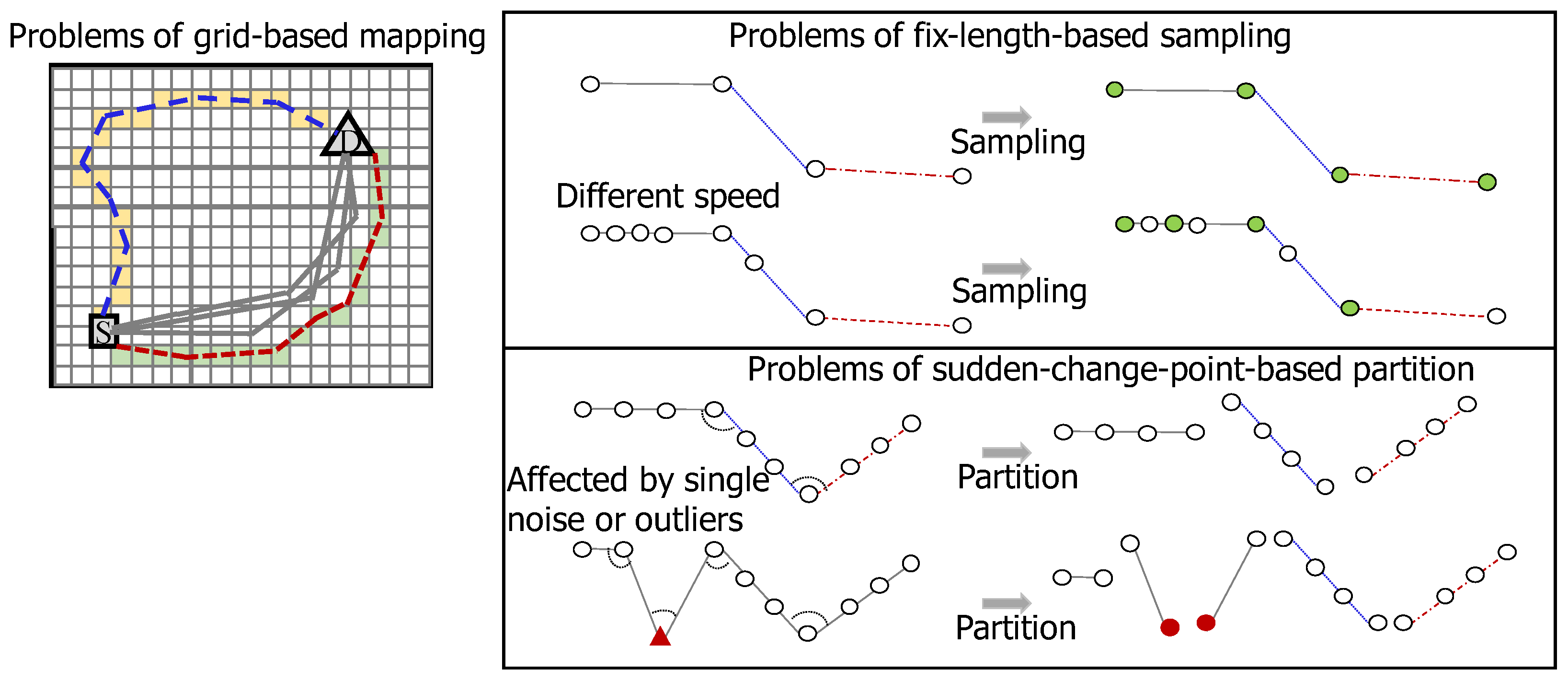
Mapping-based pre-processing methods represented a raw trajectory with a series of symbols by mapping each point in the raw trajectory into a symbol. The frequently used mapping methods were based on grid and road maps. The grid-based pre-processing method first divided the road map into grid cells of equal sizes and represented a trajectory as a sequence of traversed cell symbols in time order. It had the advantage of avoiding the effects of different sampling frequencies or traveling speeds of the moving objects. However, it had the disadvantage of being sensitive to the cell size, leading to the situation that two adjacent trajectories could be represented by two totally different sets of grid cells. For example, in Figure 3 (top left), the blue and red dash trajectories were represented by cells with a visiting frequency of one; hence, they had similar outlier scores. However, since the red dash trajectory was closer to normality, it should have a significantly different outlier score from the blue dash trajectory. The map-based pre-processing method matched the trajectory with the road map and represented a trajectory to a graph. Its disadvantages were that it was time-consuming and dependent on the road map. Hence, it could not appropriately reflect evolving road situations, such as road closures or traffic congestion.
Sampling-based pre-processing methods sample points from trajectories to obtain fixed-length sub-trajectories. The commonly used sampling methods were based on the uniform or Gaussian distribution. The disadvantage of the uniform-distribution-based sampling was that points in trajectories might not be generated evenly, which could be affected by the sampling frequency of the positioning devices or the traveling speed of the moving objects. As a result, as shown in Figure 3 (top right), two different trajectories traveling along the same road but with different numbers of points recorded in trajectories could be erroneously reflected to have different sampling results (green points). The disadvantage of the Gaussian-distribution-based sampling was that the points should follow the Gaussian distribution.
Partitioning-based pre-processing methods divided trajectory into different sub-trajectories. The typical partitioning methods were sudden-changed-point-based partition and t-partition [54]. The disadvantage of the former was the sensitivity to noise or outlier points. As shown in Figure 3 (bottom right), a noise point (red color) led to different partition results. The disadvantage of the latter was the dependency on expertise, which limited its usage in practice.
Hence, we should avoid using the pre-processing method above; however, most existing detectors still rely on these methods. Another factor was that there are few reliable trajectory outlier detectors. This might be because processing the trajectory data was very challenging and trajectory outlier detection only became a prominent area of research interest after 2000 [8].

1.6. Motivation and Contribution

To solve these two drawbacks, which are either due to the detectors themselves or the pre-processing methods utilized by the detectors, we propose a novel feature extraction technique called middle polar coordinates (MiPo). MiPo does not rely on any of the pre-processing techniques introduced above. MiPo is a feature extraction method, and each trajectory can be represented with these features in the tabular data format extracted by MiPo. Thereafter, any tabular outlier detectors, such as the detector proposed by Xu et al. [71], can be directly applied to these features to detect outliers.
The process of using MiPo and applying tabular outlier detectors is shown in Figure 2 (middle and top). Outlier detection from trajectory data and tabular data can share similar strategies in the post-processing, ensemble, and threshold components because they share similar operational units of outlier scores. For example, neighborhood averaging [72] can be used as the post-processing component to guarantee that similar objects in the feature space have similar outlier scores. Neighborhood representative [73] and regional ensemble [74] can be used as the ensemble components to combine multiple outlier scores to produce more reliable outlier scores for data objects. The two stages of median absolute deviation (MAD) [75] can be used as the threshold component [75]. However, outlier detection from the trajectory and tabular data have different strategies due to their differing inputs in the pre-processing and detector components, with the former requiring tabular data and the latter requiring trajectory data. Typical pre-processing techniques for tabular data are missing value handling, scaling, normalizing and standardizing, while typical missing pre-processing techniques for trajectory data are mapping, partitioning, and sampling. Compared with outlier detection techniques for trajectory data, outlier detection techniques for tabular data are relatively more developed, especially in the detector component, because research on tabular data commenced in the 1980s [2].
This article serves to propose a method called MiPo to extract features from trajectory data, granting tabular outlier detectors the ability to compute trajectory outliers, which was previously impossible. This article includes a comprehensive review of more than 40 trajectory outlier detection techniques published between 2000 and 2022. The source code for MiPo is provided for reproducibility, and the datasets are made available with the aim to be the first real-world public datasets with labels for trajectory outlier detection (www.OutlierNet.com).

2. Methods

This section aims to highlight the challenges faced in trajectory outlier detection before introducing MiPo, and discusses the advantages and disadvantages of MiPo.

2.1. Problem Statement

Definition 1. 
(Trajectory). A trajectory T j is defined as a series of time-ordered points: T j = { P 1 j , P 2 j , , P i j , , P m j } , where each data point P i j = ( x i j , y i j ) R 2 consists of a pair of latitude x i j and longitude y i j .
Definition 2. 
(A group of trajectories with the same source and destination ). A group of trajectories with the same source ( S = ( x s , y s ) ) and destination ( D = ( x d , y d ) ) are defined as G S , D , λ = { T 1 , T 2 , , T j , , T n } , satisfying | | P 1 j S | | λ and | | P 1 j D | | λ , where P 1 j and P 1 j are the first and last points of trajectory T j , respectively; λ R + , S, and D are given by users; | | · | | denotes the Euclidean distance.
Problem 1. 
Given a group of trajectories G S , D , λ with the same source and destination as  Figure 1(right), the objective is to find the outlier trajectories, defined as the trajectories which are few and different from other trajectories. The outlier trajectories can be sub-, entire-, or group-trajectory outliers, as illustrated in Figure 1(right). An unsupervised detector f: G S , D , λ O that outputs an outlier score O j O ( O R 1 × n ) for each input trajectory T j G S , D , λ is desired.
Challenges There are two types of challenges: data- and deployment-oriented. Data-oriented challenges include:
(1)
Processing the variable-length input;
(2)
Mitigating noise or outliers;
(3)
Addressing complicated road networks or real-time traffic.
Deployment-oriented challenges have to consider the multiple factors below:
(4)
Accuracy;
(5)
Complexity;
(6)
Robustness;
(7)
Generalizability;
(8)
Iterability;
(9)
Re-usability;
(10)
Compatibility;
(11)
Interpretability;
(12)
Scalability;
(13)
Reproducibility.
It is challenging to overcome all these challenges with a single detector. Normally, key performance indicators are application-dependent. For example, the most significant criteria will be accuracy, complexity, interpretability, and reproducibility when applying trajectory outlier detection for taxi fraud detection from large-scale data in industry. However, it will be generalizability when applying the trajectory outlier detection for mixed data, such as the mixed trajectory from humans and cars.

2.2. Middle Polar Coordinates (MiPo) for Tabular Feature Extraction from Trajectory Data

MiPo is not a coordinate but a feature extraction technique using polar coordinates. Features extracted by MiPo may be further applied in other tasks, such as clustering or outlier detection. MiPo cannot work independently for these tasks. In terms of outlier detection, existing tabular outlier detectors are employed to model the features extracted by MiPo to compute outlier scores. Therefore, our strategy for trajectory outlier detection works in two steps. In the first step, each trajectory can be represented as tabular-format features extracted from trajectory data by M i P o : T j G S , D , λ F j F . In the second step, to compute an outlier score for each represented trajectory F j F , any existing unsupervised tabular outlier detector f: F j F O j O can be employed. With this strategy, the task of detecting outliers from trajectory data using trajectory outlier detectors can be simplified to the task of detecting outliers from tabular data using tabular outlier detectors. The process of using MiPo and tabular outlier detectors is shown in Figure 2 (middle and top).
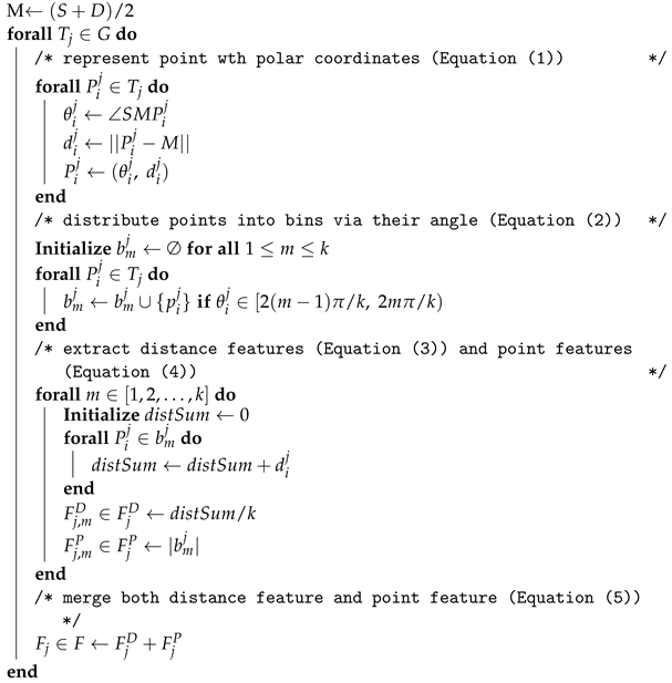
This article aims to introduce the concept of MiPo and establish the optimized configuration, which will serve as the new standard. Generally, MiPo extracts two groups of features in tabular format from trajectory data. The first group is called the distance feature and the second group is called the point feature. Given a trajectory T j G S , D , λ and for each point P i j T j , MiPo first uses polar coordinates with the reference vector M S to represent P i j = ( x i j , y i j ) as P i j = ( θ i j , d i j ) following Equation (1), where M is the middle point between S and D; the θ i j is the angle S M P i j ; and the d i j = | | P i j M | | is the Euclidean distance between the point P i j = ( x i j , y i j ) and M. MiPo then distributes points in T j into k bins with the range of 2 π / k for each according to their angles θ i j as Equation (2). For each bin b m j , the mean of d i j for all P i j b m is calculated and denoted as F j , m D F j D as shown in Equation (3). Then, the number of the points in bin b m j is counted and denoted as F j , m P F j P as shown in Equation (4). Thereby, K mean values can be obtained, which are used as the distance feature denoted as F j D . K values of point counts can also be obtained, which are used as the point feature denoted as F j P . Furthermore, these two groups of features are merged to be the final feature F j , which is used as the representation of the trajectory T j as Equation (5). Next, any tabular outlier detector can be applied to the F j to calculate the outlier score for the trajectory T j . Algorithm 1 shows the general raw idea of MiPo.
M = ( S + D ) / 2 , θ i j = S M P i j , d i j = | | P i j M | | , P i j = ( θ i j , d i j ) ,
where | | · | | denotes the Euclidean distance.
b m j = { P i j | θ i j [ 2 ( m 1 ) π / k , 2 m π / k ) ; P i j T j } , m [ 1 , k ] .
F j , m D = 1 | b m j | i = 1 | b m j | d i j , P i j b m j , F j D = [ F j , 1 D , F j , 2 D , , F j , m D , ] ,
where | · | denotes the size.
F j , m P = | b m j | F j P = [ F j , 1 P , F j , 2 P , , F j , m P , ] .
F j = [ F j , 1 D , F j , 2 D , , F j , m D , , F j , 1 P , F j , 2 P , , F j , m P , ] , F j , m D F j D , F j , m P F j P .
The general MiPo introduced above can be further optimized in different aspects. To reduce the time complexity of Algorithm 1, the first two loops in Algorithm 1 can be merged. To reduce the effect of noise or outliers caused by factors such as the GPS drifts or the positioning equipment error, the median of the distances can be used to calculate the F j , m D instead of using the mean of distances in Equation (3). It is known that the median, defined as the value separating the higher from the lower half of data, is more robust in the presence of noise or outliers than the mean [76,77,78]. Due to the different sampling frequencies or moving speeds, trajectories recorded on the same road may have different numbers of points. To reduce this effect to the point feature in Equation (3), instead of using the point counts in each bin as the point feature as shown in Equation (4), the percentage of point counts in each bin, namely F j , m D = | b m j | / | T j | , can be used for F j , m P . Since the dimensions of F j are decided by the number of the bins k and the data with a higher dimensionality may contain irrelevant or redundant information, a reduction in dimensions can be considered. To achieve this goal, feature reduction or selection techniques can be employed. However, we also propose an optimized version of MiPo, termed optimized MiPo, which incorporates the dimension reduction.
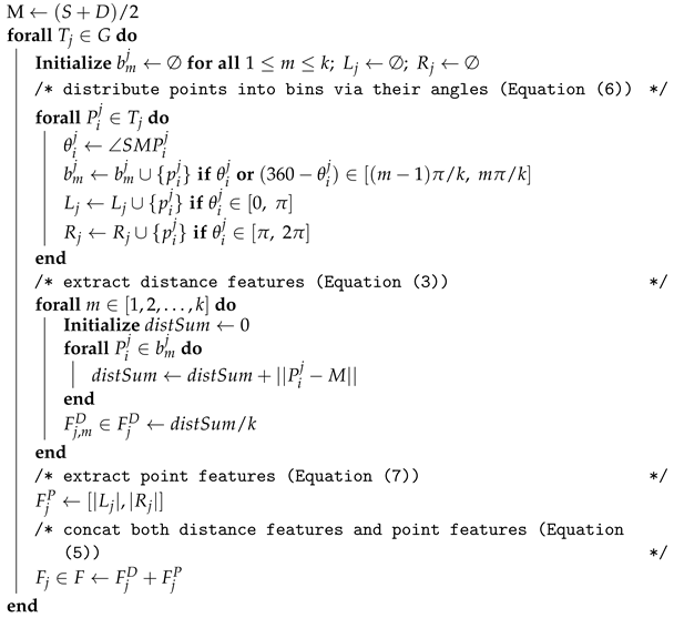
The optimized MiPo has two modifications compared with the general MiPo: the method of distributing points in Equation (2) and extracting the point feature associated with Equation (4). First, the optimized MiPo puts points which are symmetrical to the line S D into the same bin as shown in Equation (6). This optimization is based on the fact that there are rare roads in the real world that are perfectly symmetrical to the line between two places. Second, the optimized MiPo extracts the point feature considering two bins: [ 0 , π ) and [ π , 2 π ] using Equation (6). Thus, the optimized MiPo only considers the distribution of the points with respect to the line as the point feature. Considering that the distance features are more important than the point features, the weight of the point feature is lowered by reducing the dimensions of the point feature from k to 2. This optimization is helpful for the scenarios when outliers and normalities are symmetrical to the line S D . Algorithm 2 shows the optimized MiPo.    
Algorithm 1: General idea of M i P o ( G , k ) F  (Raw idea only)
Input: Trajectory dataset G with source point S and destination point D, k N +
Output: Tabular data features F
Remotesensing 14 05394 i001
Upon setting the angle range for each bin to 2 π / k , the dimension of F i obtained by the general MiPo using Algorithm 1 is 2 k , while the dimension of F i obtained by the optimized MiPo using Algorithm 2 is k / 2 + 2 . Considering the dimensions, the optimized MiPo is recommended as the standard, while the general MiPo serves to demonstrate the key idea of using polar coordinates to extract features. In the rest of the paper, the optimized MiPo will be referred to as MiPo for simplicity. Hence, Algorithm 2, instead of Algorithm 1 is the pseudocode of the proposed MiPo in this paper.
b m j = { P i j | θ i j o r ( 360 θ i j ) [ ( m 1 ) π / k , m π / k ) ; P i j T j } .
F j , 1 P = | L j | , L j = { P i j | θ i j [ 0 , π ) ; P i j T j } , F j , 2 P = | R j | , R j = { P i j | θ i j [ π , 2 π ] ; P i j T j } , F j P = [ F j , 1 P , F j , 2 P ] .
Algorithm 2:  M i P o ( G , k ) F  (Standard)
Input: Trajectory data G with source point S and destination point D, k N +
Output: Tabular data features F
Remotesensing 14 05394 i002
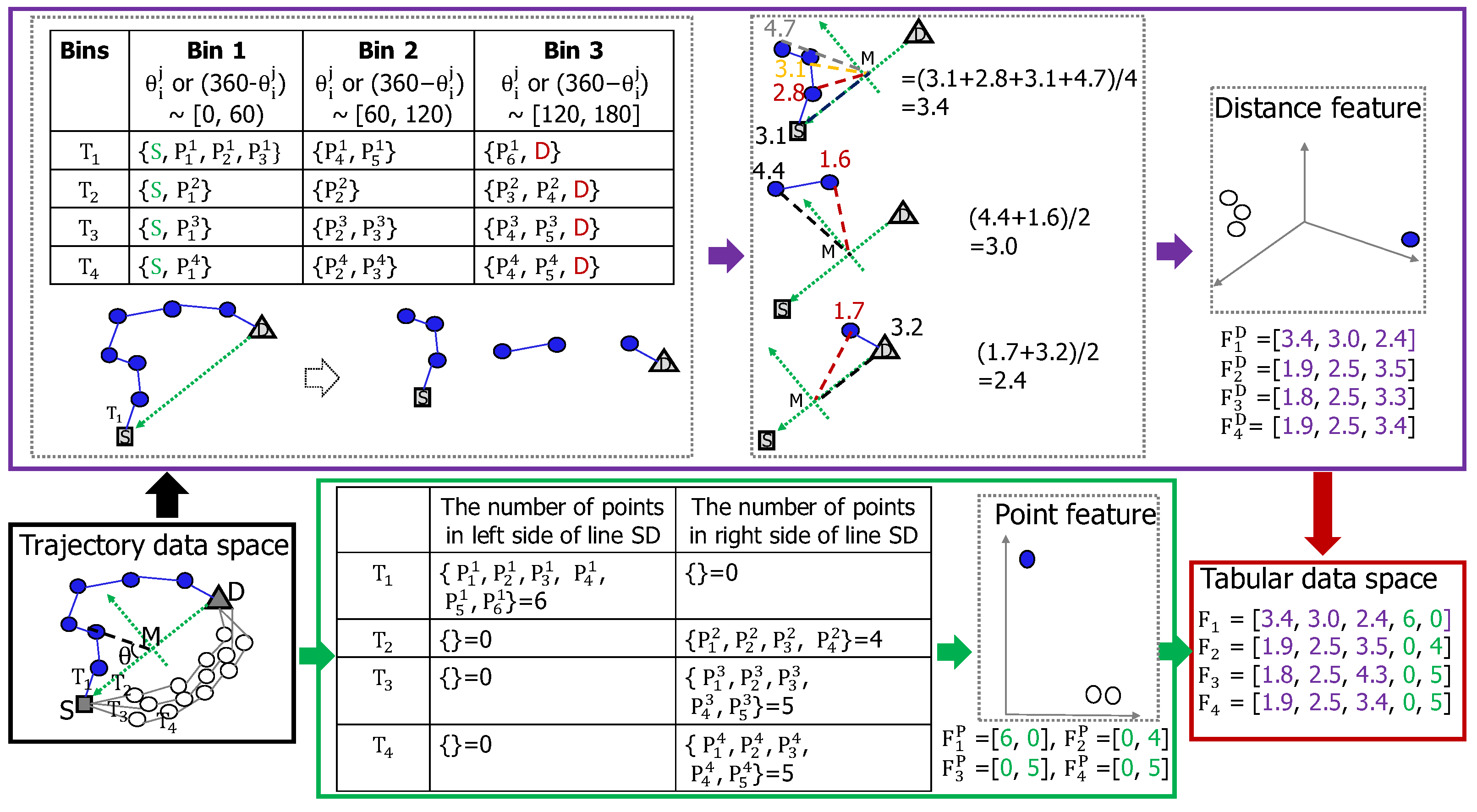
An example of applying the optimized MiPo is demonstrated in Figure 4. MiPo converts trajectory data [ T 1 , T 2 , T 3 , T 4 ] (bottom left, black rectangle box) to tabular data [ F 1 , F 2 , F 3 , F 4 ] (bottom right, red rectangle box) by extracting two groups of features from trajectory data. The first group is called the distance feature [ F 1 D , F 2 D , F 3 D , F 4 D ] (top middle, purple rectangle box) and the second group is called the point feature [ F 1 P , F 2 P , F 3 P , F 4 P ] (bottom middle, green rectangle box). To extract the distance feature, MiPo represents each point in trajectory data by using polar coordinates with the vector M S as the reference vector, where M is the middle point between the source S and destination point D. Next, the points in each trajectory are distributed into three bins as shown in the purple rectangle box. For example, the points in the trajectory T 1 are distributed into { S , P 1 1 , P 2 1 , P 3 1 } , { P 4 1 , P 5 1 } , { P 6 1 , D } . The S and D are also factored in when distributing points in each trajectory. Then, the mean of the distances between the points in Bin 1, 2, and 3 and the point M is calculated to be 3.4, 3.0, and 2.4, respectively. The distance feature of T 1 is defined as F 1 D = [ 3.4 , 3.0 , 2.4 ] . Since all six points in T 1 are located at one side of the line S D , and their angles are within the range between 0 and π , the point features of T 1 are derived to be F 1 P = [ 6 , 0 ] using Equation (7). Finally, we combine these two features to be the final features of T 1 as F 1 = [ 3.4 , 3.0 , 2.4 , 6 , 0 ] .
Once the trajectories are represented by MiPo (Algorithm 2) in tabular format, any tabular outlier detector can then be applied to compute outlier scores. This process is denoted as MiPo+, which is shown in Algorithm 3.
Algorithm 3:  M i P o + ( G , k , g ) O
Input: Trajectory data G, k N + , Tabular outlier detector g
Output: Outlier scores O
F M i P o ( G , k )
O g ( F )

2.3. MiPo-Related Discussion

Feasibility of MiPo Since all trajectories have the same source S and destination D, the significantly different places must be located between the source and destination. Therefore, the middle point M = ( S + D ) / 2 , defined as the midpoint of the source and destination, can be a potential reference point. The network of roads in the real-world space is sparse; hence, the distances between points recorded in different roads to the reference point M can make the trajectories passing different roads distinguishable. Therefore, these distances are sufficient to represent the trajectories for trajectory data mining tasks, including recognizing outliers.
Potential applications of MiPo MiPo represents trajectory data as tabular data, which can be applied to road network extraction, new roads or traffic congestion detection, road clustering, and road classification. Examples are illustrated in Section 3.8.
Related literature The concept of angle is also used by Guan et al. [64], Oehling et al. [43], Piciarelli et al. [38], and Yong et al. [17]; however, with a different definition compared with MiPo. Guan et al. [64], Oehling et al. [43], and Piciarelli et al. [38] define an angle for a point P i j T j as P i 1 j P i j P i + 1 j , while Yong et al. [17] define an angle for a point P i j T j as O P i j C , where O and C are the origin point and the centroid defined by clustering algorithms, respectively.
Disadvantage In the context of perfectly symmetrical outliers and normalities about the point M, the current MiPo (Algorithm 2) may be inadequate. However, this is a rare occurrence in the real world. To mitigate this, Equation (8) instead of Equation (7) can be used to extract the point feature.
F j , 1 P = | L T j | , L T j = { P i j | θ i j [ 0 , π / 2 ) ; P i j T j } , F j , 2 P = | R T j | , R T j = { P i j | θ i j [ π / 2 , π ) ; P i j T j } , F j , 3 P = | L B j | , L B j = { P i j | θ i j [ π , 3 π / 2 ) ; P i j T j } , F j , 4 P = | R B j | , R B j = { P i j | θ i j [ 3 π / 2 , 2 π ] ; P i j T j } , F j P = [ F j , 1 P , F j , 2 P , F j , 3 P , F j , 4 P ] .
Advantage MiPo effectively tackles most challenges listed in Section 2.1. We summarize the reasons as follows:
(1)
Processing the variable-length input: MiPo allows variable-length input;
(2)
Dealing with noise or outliers: MiPo is developed specifically for outlier detection;
(3)
Facing complicated road networks: This is verified by the experiments in Section 3;
(4)
Accuracy: This is verified by the experiments in Section 3;
(5)
Complexity: MiPo has linear time and space complexity;
(6)
Robustness: MiPo does not rely on additional parameters. MiPo is not sensitive to outliers or noise;
(7)
Generalizability: MiPo can be used for other data mining tasks as shown in Section 3.8;
(8)
Iterability: More features can be extracted from each bin defined by MiPo;
(9)
Re-usability: The feature is re-usable;
(10)
Compatibility: The feature extracted by MiPo can be jointly used with the feature extracted by other techniques;
(11)
Interpretability: The features extracted by MiPo are the distances to the point M, which is easy to understand. The outliers detected by LOF have significant density deviations from their neighbors;
(12)
Scalability: MiPo processes each trajectory without relying on other trajectories;
(13)
Reproducibility: MiPo is not a randomness-based technique.

3. Results

The experimental settings and results are detailed in this section. This section shows the datasets used, including the baselines, measurements and relevant details.

3.1. Datasets

There are no any public trajectory outlier detection datasets with labels available. Experiments were conducted based on a real-world taxi GPS trajectory dataset with the addition of labels for outliers and normalities. This dataset was downloaded from the uci.edu website (access date of 21 June 2022, with details shown in the data availability statement at the end of the paper). The dataset included 442 taxis in Porto, Portugal from 7 January 2013 to 30 June 2014, with an average GPS sampling interval of 15 s. The original dataset contains 1,710,670 trajectories.
The experiments were designed by varying different factors: the distance between the source and destination, the complexity of the road network between the source and destination, the outlier type, and the outlier ratio in the data.
  • The source and destination pair Considering the first two factors, datasets with three different source–destination pairs with the setting λ = 200 m for G S , D , λ in Definition 2 were chosen, as shown in Figure 5. The first pair was from Oporto-Francisco de Sá Carneiro Airport to Mouzinho de Albuquerque Square (Ai2Sq), with a distance of 9658 m, which was considered as a long distance. For pre-processing, trajectories with a number of GPS points between 8 and 60 were selected, which covers most trajectories. The second pair was from São Bento Train Station to Dragão Stadium (St2St), with a distance of 2878 m, which was considered as an intermediate distance. For pre-processing, trajectories with a number of the GPS points between 8 and 30 were selected, which covers most trajectories. The third pair was from University of Porto and Monument Church of St Francis (Un2Ch), with a distance of 694 m, which was considered as a short distance. For pre-processing, trajectories with a number of GPS points between 8 and 30 were selected, which covers most trajectories. To obtain these three raw datasets, trajectories from the source to destination, defined as reverse trajectories from the destination to source, were selected. Then, all trajectories were sorted to ensure that they all have the same source and destination.
  • Outlier types Three experts in outlier detection domains were employed to manually label the trajectories in these three raw datasets as either organic outliers or normalities. The final labels were decided democratically based on a voting majority of these three experts. Then, outliers are injected into these raw datasets with three different outlier generation models named d e t o u r , p e r t u r b a t i o n , and r o u t e - s w i t c h i n g , as shown in Figure 6. Similarly, these outlier generation models are also used by Zheng et al. [79], Liu et al. [25], Han et al. [24], Belhadi et al. [80], and Asma et al. [67]. The detour model created an outlier trajectory by shifting a sub-trajectory of a trajectory with a random direction and distance. The perturbation model created an outlier trajectory by moving a randomly selected point of a trajectory with a random direction and distance. The route-switching model created an outlier trajectory by connecting two sub-trajectories randomly selected from two different trajectories. Therefore, there were four types of outliers considered in the experiment: one organic outlier type and three injected outlier types.
  • Outlier ratio Two levels of outlier ratios, 5% and 10%, were considered and controlled using random sampling.
In the following, the detailed operation on the methodology of incorporating the three raw datasets to produce 12 different test datasets are described:
  • Ai2Sq Manually labeled normalities by experts were taken from the Ai2Sq raw dataset defined as the organic normalities. Six test datasets were generated as shown in Table 1 (No. 1∼6) by injecting two types of outliers:
    (1)
    Detour outlier: the shifting distance was set between 200 and 2000 m and the shifting direction was set to an angle between π / 3 and 2 π / 3 with the moving direction of the trajectory. The sub-trajectory length was between 10 % and 50 % of the entire trajectory;
    (2)
    Perturb outlier: the moving distance was set between 0 and 200 m and the moving direction was set to an angle between 0 and 2 π . A total of 60 % of points in a trajectory were moved.
  • St2St Manually labeled normalities by experts were taken from the St2St raw dataset, defined as the organic normalities. Four test datasets were generated as shown in Table 1 (No. 7∼10) by considering two types of outliers:
    (1)
    Organic outliers: manually labeled outliers by experts were taken from St2St raw dataset;
    (2)
    Route-switching outliers: A sub-trajectory starting from the source point of a trajectory and having a length ratio between 10 % and 50 % was connected to another sub-trajectory ending at the destination point of another trajectory and having a length ratio between 10 % and 50 % .
  • Un2Ch Manually labeled normalities and outliers by experts were taken from the St2St raw dataset defined as the organic normalities and outliers as shown in Table 1 (No. 11∼12).

3.2. Baselines and Evaluation

Baselines Eight trajectory outlier detectors were used as baselines: IBAT [18], IBOAT [19], RapidLOF [45], LSTM [42], ATDC [27], TPBA [67], ELSTMAE [41], and RNPAT [33]. All of them had been described in the literature review of this article. To fit the cells in the tables well in the following sections, RLOF and ELSTM were used to refer to RapidLOF and ELSTMAE, respectively.
Evaluation The area under the Receiver Operating Characteristic (ROC) curve (AUC) was employed to evaluate the performance of the detectors. The ROC curve was plotted by pairs of the true positive rate versus the false positive rate for every possible decision threshold value over outlier scores. The AUC was a value between 0 and 1, where 1 indicated a perfect detector.

3.3. AUC Comparison with Baselines

Since MiPo was not a standalone outlier detector but a feature extractor for the trajectory data, we applied the tabular outlier detector LOF [37] to the features extracted by MiPo. The LOF required a parameter n _ n e i g h b o r s , which varied from 3 to 30. The number of the bins k ranged from 3 to 60. The best AUC was reported in the first column of Table 2.
The parameters of each baseline method were also tuned, and the best AUC per baseline per dataset were reported in Table 2. RNPAT required a road map as an additional parameter to match the trajectory to the real roads. Therefore, RNPAT was applicable for the organic outlier but not applicable to injected outlier types. MiPo outperformed all baselines for all datasets, regardless of the distance or the road network between the source and destination, outlier types, or outlier ratios. MiPo had the smallest standard deviation of 0.01, showing its robustness and stability. IBAT with a 0.96 AUC was the best baseline method prior to the introduction of MiPo. Despite being the previous standard, IBAT was inferior to MiPo in some cases, such as the UnCh5M dataset with −0.13 AUC.
Hence, it was clear that MiPo consistently outperformed all baseline pre-processing methods by evaluating both accuracy and stability.

3.4. MiPo with More Tabular Outlier Detectors

MiPo was a feature extraction method that transformed the trajectory data into the tabular data; hence, the choice of the tabular detector g in Algorithm 3 could be application-dependent and not limited to the LOF [37]. In this section, we reported the results of applying various tabular detectors to the features extracted by MiPo: DOD+/ MOD+ [76], ODIN [81], NC [82], KNN [83], MCD [84], IForest [85], SVM [86], PCA [87], SOGA [88], BVAE [89], COP [90], ABOD [91], and ROD [92]. The k of MiPo was set to half of the average trajectory length, namely k= 25, 14, and 10 for the AiSq, StSt, and UnCh datasets, respectively. The parameter of n _ n e i g h b o r s was set to 15 for all k-nearest-neighbors-based detectors: DOD+/ MOD+, ODIN, NC, KNN, and ABOD. The default parameters found from the available literature were used for the remaining detectors. The experiment results were summarized in Table 3. The best average AUC performance was 0.97, which was obtained by the ABOD detector with the default parameter setting, which was still better than the best baseline trajectory outlier detector in Table 2—IBAT with the optimal parameter settings. The properties of these methods were described in Ref. [76].
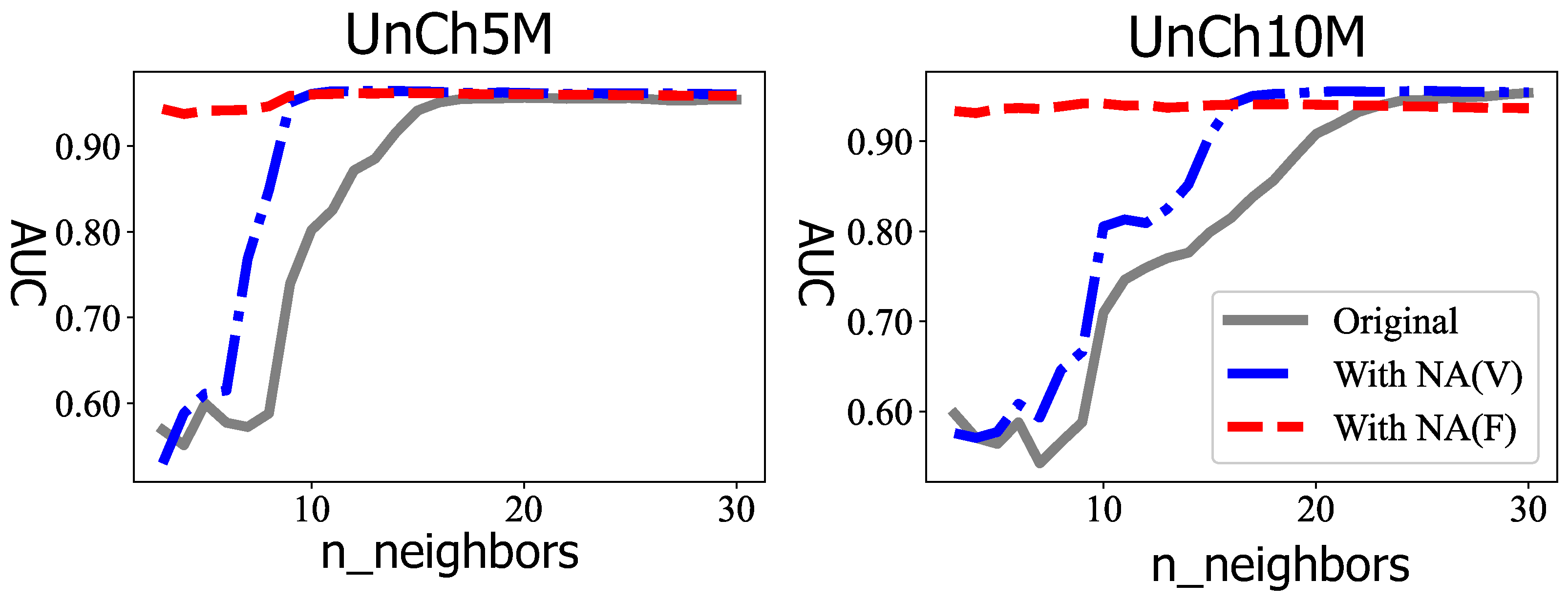
In addition, the outlier score post-processing method, such as the neighborhood average (NA) [72] or ensembles, could be applied to improve the results. NA is based on k-NN and, hence, requires a parameter n _ n e i g h b o r . When the n _ n e i g h b o r for NA was fixed to be the default value of 100 as suggested by Yang et al. [72], it was defined as NA(F). The n _ n e i g h b o r was defined as NA(V) when it was varied and set to be equal to the n _ n e i g h b o r for LOF to reduce the numbers of parameters to adjust. As shown in Figure 7, the best results were obtained by M i P o + L O F (grey solid line). However, when LOF was jointly used with NA, namely either NA(F) or NA(V), the best AUC obtained practically did not require the adjustment of parameters; yet, we obtained slightly improved results. When the original AUCs approached 0.99, NA could bring limited improvement compared with the near-perfect AUC. However, according to Yang et al. [72], NA could significantly improve a terrible detector until it attained a decent performance.
To summarize, many outlier detector techniques for tabular data became relevant once the trajectory data was represented as tabular data by MiPo due to its performance enhancements.

3.5. Effect of the Parameter k

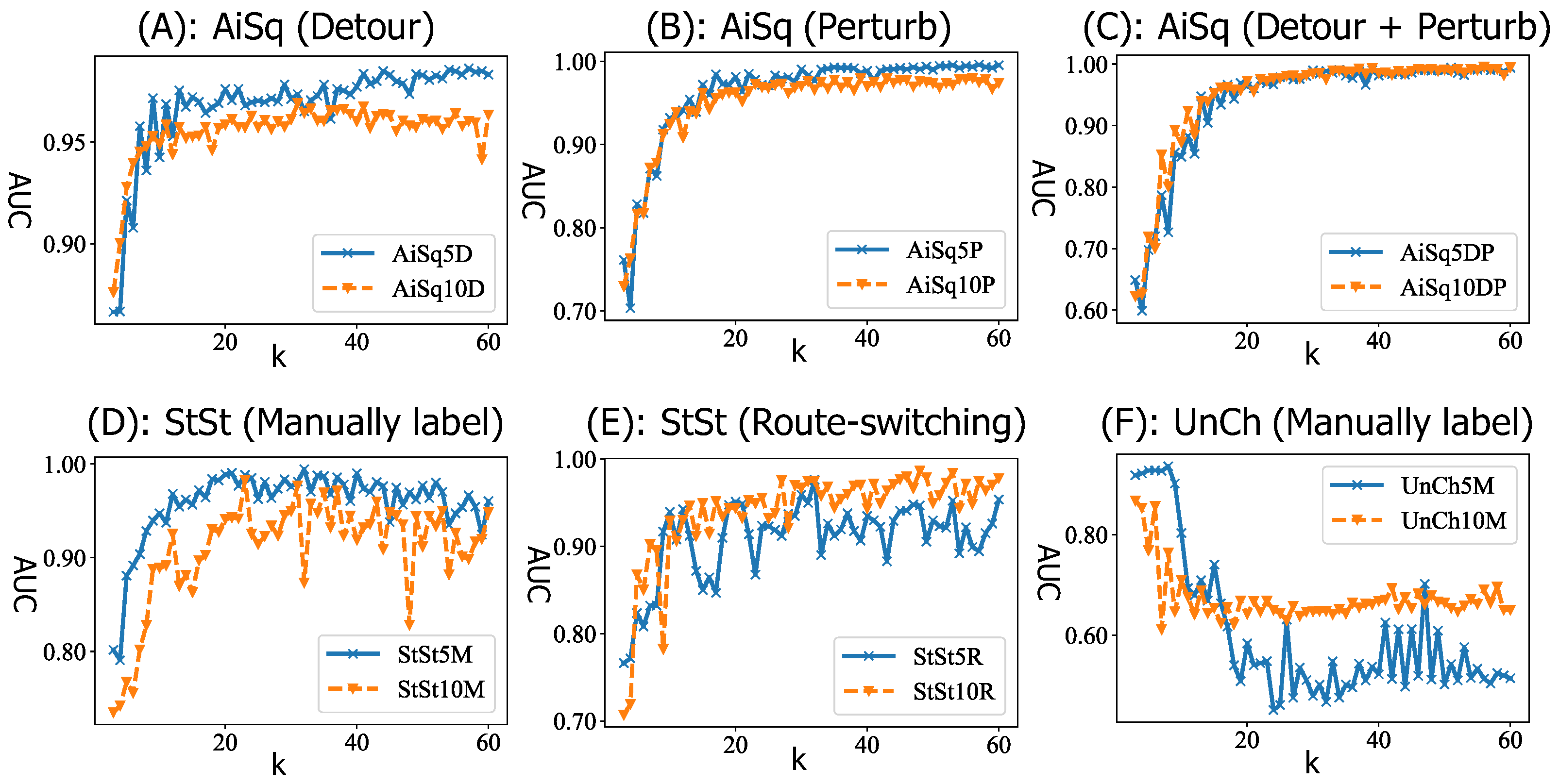
MiPo required one parameter, namely the number of the bins, which was denoted as k. M i P o + L O F was used to study the effect of k by fixing the n _ n e i g h b o r = 10 for LOF. The results were plotted in Figure 8. When the distance between the source and the destination was long, such as the AiSq and StSt datasets, a bigger k could bring better results. When the distance was short as per the UnCh dataset, a smaller k could bring better results. This indicated the optimal k was related to the distance of trajectories. It was observed that the distance between the source and the destination affects the stability of the results by visualizing the gradient of the AUC curves.
The k for MiPo was fixed to 15 to study the effect of n _ n e i g h b o r of LOF. The results are plotted in Figure 9. For the AiSq dataset, when data contained detour or perturb outliers separately, a larger n _ n e i g h b o r could bring better results. However, when data contained both outlier types concurrently, a larger n _ n e i g h b o r distorted the performance. For the StSt and UnCh datasets, with increasing n _ n e i g h b o r , the AUCs initially increased slightly, and then dropped drastically before finally steeply increasing. This might be because the LOF detector was sensitive to the distribution of the outliers with different types. Overall, this indicated that the parameters of detectors should be tuned according to the outlier types.
Another interpretation was to plot both k and n _ n e i g h b o r on the same diagram as shown in Figure 10. This led to two important deductions. First, good results (yellow color) were always obtained when both k and n _ n e i g h b o r were larger. Second, the distance between the source and the destination affected the stability of the results by visualizing the scatters of points.
In summary, MiPo relied on detectors to produce outlier scores; hence, the parameters of MiPo and the detectors should be jointly tuned at the same time. When LOF was used, larger values for both k and n _ n e i g h b o r were recommended. When the optimal k for MiPo was considered, the trajectory length was an important factor. According to Section 3.5, when setting k to be half of the average trajectory length and using the default parameters for tabular detectors, a good result with the 0.97 AUC could still be obtained (by ABOD). Therefore, this result suggested setting k to be half of the average trajectory length as the default. The experiment also showed that for a long-distance trajectory dataset, such as the AiSq, k values larger than 30 did not bring much more improvement. Thus, k was recommended to be 30 at maximum.

3.6. Time Complexity

The running times of MiPo-, MiPo, MiPo+LOF, and other trajectory outlier detection methods with varying n and m were summarized in Table 4 and illustrated in Figure 11. All methods were implemented in Python and ran on a computer with an Intel Core i7-11700 CPU. Figure 11 showed that the time complexity of MiPo was linearly related to both n and m.
MiPo- referred to the situation where all the points in trajectories were stored in the database in advance using the format of polar coordinates with the reference vector of M S , instead of the GPS point format shown in Figure 12. Thus, MiPo’s computing time could be reduced by optimizing the data format in the database. MiPo+LOF denoted the time of applying both MiPo and the LOF detector. In summary, MiPo- and MiPo outputted the same features but differed in how the GPS trajectories were stored in the database. MiPo+ outputted outlier scores computed by tabular outlier detectors, such as LOF, via modeling the features extracted by MiPo. Their differences were shown in Figure 12.
As shown in Table 4, MiPo- required approximately 0.79 s to extract features for 10,000 of trajectories with lengths of 90, averaging 1 μs for each trajectory. MiPo required an average of 2.7 ms to extract features for each trajectory. This demonstrated MiPo’s efficiency and emphasized the potential of further reductions in computational time if the data were appropriately formatted.
The advantages of the proposed method were evident upon the comparison of MiPO+LOF with other trajectory outlier detection methods. For example, compared with IBAT, which was the most competitive method in terms of accuracy, MiPo+LOF required approximately 10% of IBAT’s running time. The fastest method was RapidLOF; however, the increased speed compromised accuracy, as shown in the column of RapidLOF in Table 4. Compared with deep learning-based methods, such as LSTM and ELSTMAE, MiPo+LOF was more than 40 times faster. The slowest detector was RNPAT due to its complex map-matching pre-processing method.
To sum up, MiPo+LOF was an efficient method, optimizing speed and accuracy when compared with other baseline methods. Apart from its stellar performance, it could be further improved by optimizing data storage.

3.7. Potential Applications

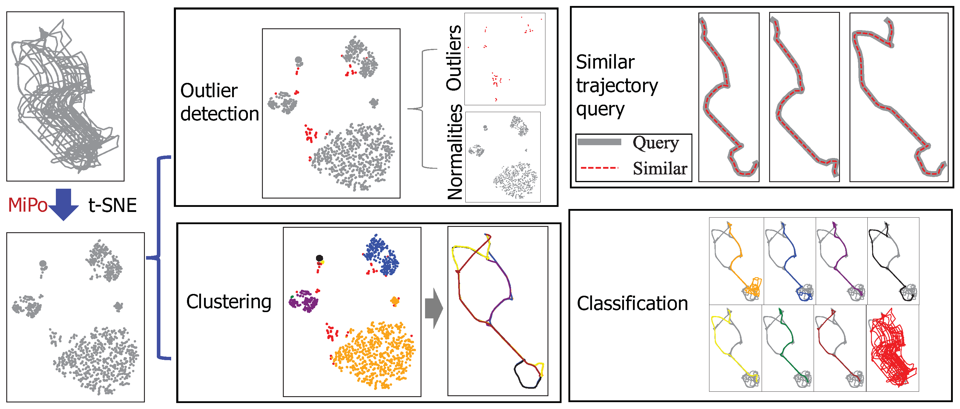
The feature extracted by MiPo could be used for other trajectory data mining applications as well such as clustering, classification, and similar trajectory searching, as shown in Figure 13 with the AiSq5D dataset. The task of clustering trajectories could be performed by clustering the features extracted from the trajectories by MiPo as shown on the bottom left in Figure 13. The task of classifying trajectories could be performed by classifying the features extracted from the trajectories by MiPo as shown in the bottom left in Figure 13. The task of searching the similar trajectories of a given trajectory could be performed by searching the similar features extracted from the trajectories by MiPo as shown in the top right of Figure 13. Since this paper focused on outlier detection, further discussion on this topic would be future work.

3.8. Limitation

Apart from the disadvantages of MiPo mentioned in Section 2.3, MiPo might be less effective as a distance-based method when the trajectories are recorded in a space with a very dense road network. However, most road networks in the real world are not dense. Moreover, MiPo relied on other detectors to produce outlier scores. The limitation of the detectors utilized might affect the performance of outlier detection when using MiPo.

4. Discussion

Although trajectory outlier detection had been developed since 2000, the literature addressing effective deployment methods in the industry is scarce. Multiple factors should be considered when developing trajectory outlier detectors for large-scale data in industry settings. The problem of trajectory outlier detection is defined with a source and destination pair (SD pair). Supposing a city contains v SD pairs, the cost for a single SD pair will require v times more, including:
  • The time for pre-processing data;
  • The storage for the pre-processed data;
  • The time for outlier detectors’ training, storing, and updating;
  • The time and memory for outlier detectors’ predictions.
Therefore, a cost-efficient solution is normally what the industry seeks. Our solution posed a question to the domain of trajectory data mining: is a complex solution needed for the trajectory data mining of large-scale data in the industry? By virtue that the road network is sparse, MiPo has significant advantages as mentioned in Section 2.3, with the tabular outlier detector LOF in the detection of trajectory outliers measuring 0.99 AUC on average, requiring approximately 10% processing time compared with the most competitive baseline IBAT. For storage, IBAT represented each trajectory using cells with a size of 200 meters. For the AiSq dataset with 9658 meters between the source and destination, IBAT required around 50 cells for each trajectory, which was the minimum number calculated by the shortest trajectory between the source and destination. However, MiPo required only 25 numbers at most, which was half of IBAT, and this can be further reduced by dimension reduction techniques, such as t-SNE. IBAT was based on the random forests; hence, its outcome was not always reliable. However, MiPo did not suffer from this limitation.

5. Conclusions

We proposed a method called MiPo for trajectory outlier detection. MiPo represented each trajectory with tabular features. The techniques for the tabular data mining tasks, such as outlier detection, clustering, classification, and similar trajectory searching, could then be applied to these features. The trajectory outlier detection experiments with the real-world dataset showed that with the tabular outlier detector LOF, MiPo outperformed all baselines with merely approximately 10% of the computing time of the previously best performing method. MiPo has many advantages, making it suitable for industrial applications and online deployment.
A future avenue of research could be to cooperate with enterprises in the transportation industry to perform online tests by combining MiPo with different applications, such as outlier detection, clustering, classification and similar trajectory searching, and report the results. In addition, future considerations include representing each trajectory without relying on local information, namely the vector M S .

Author Contributions

Conceptualization, J.Y. and X.T.; methodology, J.Y.; software, J.Y. and X.T.; validation, J.Y., X.T. and S.R.; formal analysis, J.Y., X.T. and S.R.; investigation, J.Y., X.T. and S.R.; data curation, X.T.; writing—original draft preparation, J.Y.; writing—review and editing, J.Y., X.T. and S.R.; visualization, J.Y. and X.T.. All authors have read and agreed to the published version of the manuscript.

Funding

This research received no external funding.

Informed Consent Statement

Not applicable.

Data Availability Statement

Original raw taxi data with access date of 21 June 2022: https://archive.ics.uci.edu/ml/datasets.php. Links for the codes and labeled datasets: www.OutlierNet.com.

Conflicts of Interest

The authors declare no conflict of interest.

Appendix A

Table A1. Advantages and disadvantages of trajectory outlier detectors introduced in Section 1 and the proposed MiPo.
MethodPre-ProcessingAdvantagesDisadvantages
TOP-EYE
[17], 2010
MappingReduction in false positive rates and capturing the evolving nature of abnormal moving trajectoriesToo sensitive to its own parameters
iBAT
[18], 2011
MappingLinear time complexityPoor accuracy for cluster outliers
iBOAT
[19], 2013
MappingReal-time evaluation of outliers for active trajectoriesSensitive to noise or point outliers
iBDD
[20], 2015
MappingReal-time detection of outliersLimited to detection of disoriented behaviors of cognitively-impaired elders
MT-MAD
[21], 2016
MappingProcessing trajectories with uncertainty (i.e., trajectories not restricted by road network)Being limited to the application of maritime vessels
MCAT
[22], 2021
MappingReal-time detection of outliersAdditional parameter required: Time
Ge et al.
[23], 2011
MappingReal-time detection of outliersLimited to taxi fraud detection
DeepTEA
[24], 2022
MappingScalabilityLimited to vehicles
Additional parameter required: Time
GM-VSAE
[25], 2020
MappingScalabilityToo sensitive to its own parameters
TPRO
[26], 2015
MappingDetection of time-dependent outliersAdditional parameter required: Time
Inability to detect non-time-dependent outliers
ATDC
[27], 2020
MappingAnalysis of different anomalous patternsHigh time complexity
RPat
[29], 2013
MappingEvaluation of real-time trajectoriesLimited to video surveillance applications
Additional parameter required: Traffic flow rate
Detect
[30], 2014
MappingDetection of traffic-based outliersAdditional parameter required: Time
MANTRA
[31], 2016
MappingScalabilityAdditional parameter required: Time
DB-TOD
[32], 2017
MappingDetection of outliers in an early stageLimited to vehicles
Additional parameter required: Road map
RNPAT
[33], 2022
MappingInterpretability of the judgment for outliersHigh time complexity
Additional parameter required: Road map
LoTAD
[36], 2018
MappingInterpretability of the judgment for outliersHigh time complexity
Additional parameter required: Road map
Piciarelli et al.
[38], 2008
SamplingInterpretability of the judgment for outliersHigh time complexity
Masciari
[39], 2011
SamplingInterpretability of the judgment for outliersHigh time complexity
Maleki et al.
[41], 2021
SamplingRobust performance in the presence of noise or outliersLow scability
Oehling et al.
[43], 2019
SamplingInterpretability of the judgment for outliersHigh time complexity
Limited to flight trajectories
RapidLOF
[45], 2019
SamplingLow time complexity
Interpretability of the judgment for outliers
Low generality to other outlier types
PN-Opt
[48], 2014
SamplingInterpretability of the judgment for outliersHigh time complexity
Yu et al.
[49], 2017
SamplingInterpretability of the judgment for outliersHigh time complexity
Ando et al.
[50], 2015
SamplingBeing relatively robust even in the presence of noise or outliersHigh time complexity
Maiorano et al.
[51], 2016
SamplingInterpretability of the judgment for outliersHigh time complexity
Additional parameter required: Time
STN-Outlier
[53], 2018
SamplingInterpretability of the judgment for outliersHigh time complexity
TRAOD
[54], 2008
PartitioningInterpretability of the judgment for outliersHeavy reliance on expert knowledge to tune parameters
Luan et al.
[55], 2017
PartitioningInterpretability of the judgment for outliersHeavy reliance on expert knowledge to tune parameters
Pulshashi et al.
[56], 2018
PartitioningInterpretability of the judgment for outliersHeavy reliance on expert knowledge to tune parameters
CTOD
[57], 2009
PartitioningRecognition of new clusters to aid in identification of new roadsHigh time complexity
RTOD
[59], 2012
PartitioningInterpretability of the judgment for outliersHigh time complexity
TODS
[60], 2017
PartitioningDetection of outliers regardless of distance to the clustersHigh time complexity
F-DBSCAN
[61], 2018
PartitioningInterpretability of the judgment for outliersHigh time complexity
TODCSS
[62], 2018
PartitioningInterpretability of the judgment for outliersHigh time complexity
CaD
[63], 2019
PartitioningInterpretability of the judgment for outliersBeing limited to video surveillance
TOD-SS
[64], 2011
PartitioningInterpretability of the judgment for outliersHigh time complexity
TAD-FD
[65], 2020
PartitioningInterpretability of the judgment for outliersHigh time complexity
STC
[66], 2021
PartitioningInterpretability of the judgment for outliersLimited to taxis
Additional parameter required: Time
TPBA
[67], 2020
PartitioningInterpretability of the judgment for outliersHigh time complexity
TCATD
[68], 2018
-Interpretability of the judgment for outliersBeing sensitive to noise or outliers
OFF-ATPD
[69], 2021
-Detection of traffic-based outliersLimited to bus
Additional parameter required: Time, velocity
TODDT
[70], 2020
-Interpretability of the judgment for outliersLimited to ship
Additional parameter required: Time
MiPo
proposed,2022
-See Section 2.3See Section 2.3

References

  1. Meng, F.; Yuan, G.; Lv, S.; Wang, Z.; Xia, S. An overview on trajectory outlier detection. Artif. Intell. Rev. 2019, 52, 2437–2456. [Google Scholar] [CrossRef]
  2. Hawkins, D.M. Identification of Outliers; Springer: Dordrecht, The Netherlands, 1980; Volume 11. [Google Scholar]
  3. Yang, J.; Rahardja, S.; Rahardja, S. Click fraud detection: HK-index for feature extraction from variable-length time series of user behavior. In Proceedings of the Machine Learning for Signal Processing, Xi’an, China, 22–24 August 2022. [Google Scholar]
  4. Aggarwal, C.C. An introduction to outlier analysis. In Outlier Analysis; Springer: Dordrecht, The Netherlands, 2017; pp. 1–34. [Google Scholar]
  5. Alowayr, A.D.; Alsalooli, L.A.; Alshahrani, A.M.; Akaichi, J. A Review of Trajectory Data Mining Applications. In Proceedings of the 2021 International Conference of Women in Data Science at Taif University (WiDSTaif), Riyadh, Saudi Arabia, 30–31 March 2021; pp. 1–6. [Google Scholar]
  6. Cui, H.; Wu, L.; Hu, S.; Lu, R.; Wang, S. Recognition of urban functions and mixed use based on residents’ movement and topic generation model: The case of Wuhan, China. Remote Sens. 2020, 12, 2889. [Google Scholar] [CrossRef]
  7. Qian, Z.; Liu, X.; Tao, F.; Zhou, T. Identification of urban functional areas by coupling satellite images and taxi GPS trajectories. Remote Sens. 2020, 12, 2449. [Google Scholar] [CrossRef]
  8. Knorr, E.M.; Ng, R.T.; Tucakov, V. Distance-based outliers: Algorithms and applications. Vldb J. 2000, 8, 237–253. [Google Scholar] [CrossRef]
  9. Porikli, F. Trajectory pattern detection by hmm parameter space features and eigenvector clustering. In Proceedings of the 8th European Conference on Computer Vision, Prague, Czech Republic, 11–14 May 2004. [Google Scholar]
  10. Stauffer, C.; Grimson, W.E.L. Learning patterns of activity using real-time tracking. IEEE Trans. Pattern Anal. Mach. Intell. 2000, 22, 747–757. [Google Scholar] [CrossRef] [Green Version]
  11. D’Urso, P. Fuzzy clustering for data time arrays with inlier and outlier time trajectories. IEEE Trans. Fuzzy Syst. 2005, 13, 583–604. [Google Scholar] [CrossRef]
  12. Piciarelli, C.; Foresti, G.L. On-line trajectory clustering for anomalous events detection. Pattern Recognit. Lett. 2006, 27, 1835–1842. [Google Scholar] [CrossRef]
  13. Piciarelli, C.; Foresti, G.L. Anomalous trajectory detection using support vector machines. In Proceedings of the 2007 IEEE Conference on Advanced Video and Signal Based Surveillance, London, UK, 5–7 September 2007; pp. 153–158. [Google Scholar]
  14. Bradley, P.S.; Fayyad, U.M.; Reina, C.A.; Bradley, F.R.; Bradley, P.; Fayyad, U.; Reina, C. Scaling Clustering Algorithms to Large Databases”, Microsoft Research Report 1998. Available online: http://www.it.uu.se/edu/course/homepage/infoutv2/vt13/tr-98-37.pdf (accessed on 21 June 2022).
  15. Keogh, E.; Chakrabarti, K.; Pazzani, M.; Mehrotra, S. Locally adaptive dimensionality reduction for indexing large time series databases. In Proceedings of the 2001 ACM SIGMOD International Conference on Management of Data, California, CA, USA, 21–24 May 2001; pp. 151–162. [Google Scholar]
  16. Chu, S.; Keogh, E.; Hart, D.; Pazzani, M. Iterative deepening dynamic time warping for time series. In Proceedings of the 2002 SIAM International Conference on Data Mining, Arlington, VA, USA, 11–13 April 2002; pp. 195–212. [Google Scholar]
  17. Ge, Y.; Xiong, H.; Zhou, Z.h.; Ozdemir, H.; Yu, J.; Lee, K.C. Top-eye: Top-k evolving trajectory outlier detection. In Proceedings of the 19th ACM International Conference on Information and Knowledge Management, Toronto, Canada, 26–30 October 2010; pp. 1733–1736. [Google Scholar]
  18. Zhang, D.; Li, N.; Zhou, Z.H.; Chen, C.; Sun, L.; Li, S. iBAT: Detecting anomalous taxi trajectories from GPS traces. In Proceedings of the 13th International Conference on Ubiquitous Computing, Beijing, China, 17–21 September 2011; pp. 99–108. [Google Scholar]
  19. Chen, C.; Zhang, D.; Castro, P.S.; Li, N.; Sun, L.; Li, S.; Wang, Z. iBOAT: Isolation-based online anomalous trajectory detection. IEEE Trans. Intell. Transp. Syst. 2013, 14, 806–818. [Google Scholar] [CrossRef]
  20. Lin, Q.; Zhang, D.; Connelly, K.; Ni, H.; Yu, Z.; Zhou, X. Disorientation detection by mining GPS trajectories for cognitively-impaired elders. Pervasive Mob. Comput. 2015, 19, 71–85. [Google Scholar] [CrossRef]
  21. Lei, P.R. A framework for anomaly detection in maritime trajectory behavior. Knowl. Inf. Syst. 2016, 47, 189–214. [Google Scholar] [CrossRef]
  22. Chen, D.; Du, Y.; Xu, S.; Sun, Y.E.; Huang, H.; Gao, G. Online Anomalous Taxi Trajectory Detection Based on Multidimensional Criteria. In Proceedings of the 2021 International Joint Conference on Neural Networks (IJCNN), Shenzhen, China, 18–22 July 2021; pp. 1–8. [Google Scholar]
  23. Ge, Y.; Xiong, H.; Liu, C.; Zhou, Z.H. A taxi driving fraud detection system. In Proceedings of the 2011 IEEE 11th International Conference on Data Mining, Vancouver, Canada, 11–14 December 2011; pp. 181–190. [Google Scholar]
  24. Han, X.; Cheng, R.; Ma, C.; Grubenmann, T. DeepTEA: Effective and efficient online time-dependent trajectory outlier detection. Proc. Vldb Endow. 2022, 15, 1493–1505. [Google Scholar] [CrossRef]
  25. Liu, Y.; Zhao, K.; Cong, G.; Bao, Z. Online anomalous trajectory detection with deep generative sequence modeling. In Proceedings of the 2020 IEEE 36th International Conference on Data Engineering (ICDE), Dallas, TX, USA, 20–24 April 2020; pp. 949–960. [Google Scholar]
  26. Zhu, J.; Jiang, W.; Liu, A.; Liu, G.; Zhao, L. Time-dependent popular routes based trajectory outlier detection. In Proceedings of the International Conference on Web Information Systems Engineering, Miami, FL, USA, 1–3 November 2015; pp. 16–30. [Google Scholar]
  27. Wang, J.; Yuan, Y.; Ni, T.; Ma, Y.; Liu, M.; Xu, G.; Shen, W. Anomalous trajectory detection and classification based on difference and intersection set distance. IEEE Trans. Veh. Technol. 2020, 69, 2487–2500. [Google Scholar] [CrossRef]
  28. Lou, Y.; Zhang, C.; Zheng, Y.; Xie, X.; Wang, W.; Huang, Y. Map-matching for low-sampling-rate GPS trajectories. In Proceedings of the 17th ACM SIGSPATIAL International Conference on Advances in Geographic Information Systems, Miami, FL, USA, 1–3 November 2009; pp. 352–361. [Google Scholar]
  29. Saleem, M.A.; Nawaz, W.; Lee, Y.K.; Lee, S. Road segment partitioning towards anomalous trajectory detection for surveillance applications. In Proceedings of the 2013 IEEE 14th International Conference on Information Reuse &Integration (IRI), San Francisco, CA, USA, 14–16 August 2013; pp. 610–617. [Google Scholar]
  30. Lan, J.; Long, C.; Wong, R.C.W.; Chen, Y.; Fu, Y.; Guo, D.; Liu, S.; Ge, Y.; Zhou, Y.; Li, J. A new framework for traffic anomaly detection. In Proceedings of the 2014 SIAM International Conference on DATA MINING, Philadelphia, PA, USA, 24–26 April 2014; pp. 875–883. [Google Scholar]
  31. Banerjee, P.; Yawalkar, P.; Ranu, S. Mantra: A scalable approach to mining temporally anomalous sub-trajectories. In Proceedings of the 22nd ACM SIGKDD International Conference on Knowledge Discovery and Data Mining, San Francisco, CA, USA, 13–17 August 2016; pp. 1415–1424. [Google Scholar]
  32. Wu, H.; Sun, W.; Zheng, B. A fast trajectory outlier detection approach via driving behavior modeling. In Proceedings of the 2017 ACM on Conference on Information and Knowledge Management, Singapore, 6–10 November 2017; pp. 837–846. [Google Scholar]
  33. Zhao, X.; Su, J.; Cai, J.; Yang, H.; Xi, T. Vehicle anomalous trajectory detection algorithm based on road network partition. Appl. Intell. 2022, 52, 8820–8838. [Google Scholar] [CrossRef]
  34. Dijkstra, E.W. A note on two problems in connexion with graphs. Numer. Math. 1959, 1, 269–271. [Google Scholar] [CrossRef] [Green Version]
  35. Qin, K.; Wang, Y.; Wang, B. Detecting anomalous trajectories using the Dempster-Shafer evidence theory considering trajectory features from taxi GNSS data. Information 2018, 9, 258. [Google Scholar] [CrossRef] [Green Version]
  36. Kong, X.; Song, X.; Xia, F.; Guo, H.; Wang, J.; Tolba, A. LoTAD: Long-term traffic anomaly detection based on crowdsourced bus trajectory data. World Wide Web 2018, 21, 825–847. [Google Scholar] [CrossRef]
  37. Breunig, M.M.; Kriegel, H.P.; Ng, R.T.; Sander, J. LOF: Identifying density-based local outliers. In Proceedings of the 2000 ACM SIGMOD International Conference on Management of Data, Dallas, TX, USA, 16–18 May 2000; pp. 93–104. [Google Scholar]
  38. Piciarelli, C.; Micheloni, C.; Foresti, G.L. Trajectory-based anomalous event detection. IEEE Trans. Circuits Syst. Video Technol. 2008, 18, 1544–1554. [Google Scholar] [CrossRef]
  39. Masciari, E. Trajectory outlier detection using an analytical approach. In Proceedings of the 2011 IEEE 23rd International Conference on Tools with Artificial Intelligence, Boca Raton, FL, USA, 7–9 November 2011; pp. 377–384. [Google Scholar]
  40. Secker, A.; Taubman, D. Lifting-based invertible motion adaptive transform (LIMAT) framework for highly scalable video compression. IEEE Trans. Image Process. 2003, 12, 1530–1542. [Google Scholar] [CrossRef] [Green Version]
  41. Maleki, S.; Maleki, S.; Jennings, N.R. Unsupervised anomaly detection with LSTM autoencoders using statistical data-filtering. Appl. Soft Comput. 2021, 108, 107443. [Google Scholar] [CrossRef]
  42. Hochreiter, S.; Schmidhuber, J. Long short-term memory. Neural Comput. 1997, 9, 1735–1780. [Google Scholar] [CrossRef]
  43. Oehling, J.; Barry, D.J. Using machine learning methods in airline flight data monitoring to generate new operational safety knowledge from existing data. Saf. Sci. 2019, 114, 89–104. [Google Scholar] [CrossRef]
  44. Kriegel, H.P.; Kröger, P.; Schubert, E.; Zimek, A. LoOP: Local outlier probabilities. In Proceedings of the 18th ACM conference on Information and knowledge management, Hong Kong, China, 2–6 November 2009; pp. 1649–1652. [Google Scholar]
  45. Yang, J.; Mariescu-Istodor, R.; Fränti, P. Three rapid methods for averaging GPS segments. Appl. Sci. 2019, 9, 4899. [Google Scholar] [CrossRef] [Green Version]
  46. Arasu, A.; Babu, S.; Widom, J. The CQL continuous query language: Semantic foundations and query execution. Vldb J. 2006, 15, 121–142. [Google Scholar] [CrossRef]
  47. Liu, H.; Taniguchi, T.; Tanaka, Y.; Takenaka, K.; Bando, T. Visualization of driving behavior based on hidden feature extraction by using deep learning. IEEE Trans. Intell. Transp. Syst. 2017, 18, 2477–2489. [Google Scholar] [CrossRef]
  48. Yu, Y.; Cao, L.; Rundensteiner, E.A.; Wang, Q. Detecting moving object outliers in massive-scale trajectory streams. In Proceedings of the 20th ACM SIGKDD International Conference on Knowledge Discovery and Data Mining, New York, NY, USA, 24–27 August 2014; pp. 422–431. [Google Scholar]
  49. Yu, Y.; Cao, L.; Rundensteiner, E.A.; Wang, Q. Outlier detection over massive-scale trajectory streams. ACM Trans. Database Syst. (Tods) 2017, 42, 1–33. [Google Scholar] [CrossRef]
  50. Ando, S.; Thanomphongphan, T.; Seki, Y.; Suzuki, E. Ensemble anomaly detection from multi-resolution trajectory features. Data Min. Knowl. Discov. 2015, 29, 39–83. [Google Scholar] [CrossRef]
  51. Maiorano, F.; Petrosino, A. Granular trajectory based anomaly detection for surveillance. In Proceedings of the 2016 23rd International Conference on Pattern Recognition (ICPR), Cancún, Mexico, 4–8 December 2016; pp. 2066–2072. [Google Scholar]
  52. Albanese, A.; Pal, S.K.; Petrosino, A. Rough sets, kernel set, and spatiotemporal outlier detection. IEEE Trans. Knowl. Data Eng. 2012, 26, 194–207. [Google Scholar] [CrossRef]
  53. Zhu, Z.; Yao, D.; Huang, J.; Li, H.; Bi, J. Sub-trajectory-and trajectory-neighbor-based outlier detection over trajectory streams. In Proceedings of the Pacific-Asia Conference on Knowledge Discovery and Data Mining, Melbourne, VIC, Australia, 3–6 June 2018; pp. 551–563. [Google Scholar]
  54. Lee, J.G.; Han, J.; Li, X. Trajectory outlier detection: A partition-and-detect framework. In Proceedings of the 2008 IEEE 24th International Conference on Data Engineering, Cancún, Mexico, 7–12 April 2008; pp. 140–149. [Google Scholar]
  55. Luan, F.; Zhang, Y.; Cao, K.; Li, Q. Based local density trajectory outlier detection with partition-and-detect framework. In Proceedings of the 2017 13th International Conference on Natural Computation, Fuzzy Systems and Knowledge Discovery (ICNC-FSKD), Guilin, China, 29–31 July 2017; pp. 1708–1714. [Google Scholar]
  56. Pulshashi, I.R.; Bae, H.; Choi, H.; Mun, S. Smoothing of trajectory data recorded in harsh environments and detection of outlying trajectories. In Proceedings of the 7th International Conference on Emerging Databases, Melbourne, VIC, Australia, 3–6 June 2018; pp. 89–98. [Google Scholar]
  57. Ying, X.; Xu, Z.; Yin, W.G. Cluster-based congestion outlier detection method on trajectory data. In Proceedings of the 2009 Sixth International Conference on Fuzzy Systems and Knowledge Discovery, Tianjin, China, 14–16 August 2009; Volume 5, pp. 243–247. [Google Scholar]
  58. Ester, M.; Kriegel, H.P.; Sander, J.; Xu, X. A density-based algorithm for discovering clusters in large spatial databases with noise. In Proceedings of the Second International Conference on Knowledge Discovery and Data Mining, Portland, Oregon, 2–4 August 1996; Volume 96, pp. 226–231. [Google Scholar]
  59. Liu, L.; Qiao, S.; Zhang, Y.; Hu, J. An efficient outlying trajectories mining approach based on relative distance. Int. J. Geogr. Inf. Sci. 2012, 26, 1789–1810. [Google Scholar] [CrossRef]
  60. Mao, J.; Wang, T.; Jin, C.; Zhou, A. Feature grouping-based outlier detection upon streaming trajectories. IEEE Trans. Knowl. Data Eng. 2017, 29, 2696–2709. [Google Scholar] [CrossRef]
  61. Zhang, T.; Zhao, S.; Chen, J. Ship trajectory outlier detection service system based on collaborative computing. In Proceedings of the 2018 IEEE World Congress on Services (SERVICES), San Francisco, CA, USA, 2–7 July 2018; pp. 15–16. [Google Scholar]
  62. Yu, Q.; Luo, Y.; Chen, C.; Wang, X. Trajectory outlier detection approach based on common slices sub-sequence. Appl. Intell. 2018, 48, 2661–2680. [Google Scholar] [CrossRef]
  63. San Román, I.; Martín de Diego, I.; Conde, C.; Cabello, E. Outlier trajectory detection through a context-aware distance. Pattern Anal. Appl. 2019, 22, 831–839. [Google Scholar] [CrossRef]
  64. Yuan, G.; Xia, S.; Zhang, L.; Zhou, Y.; Ji, C. Trajectory outlier detection algorithm based on structural features. J. Comput. Inf. Syst. 2011, 7, 4137–4144. [Google Scholar]
  65. Wang, Z.; Yuan, G.; Pei, H.; Zhang, Y.; Liu, X. Unsupervised learning trajectory anomaly detection algorithm based on deep representation. Int. J. Distrib. Sens. Netw. 2020, 16, 1550147720971504. [Google Scholar] [CrossRef]
  66. Kong, X.; Zhu, B.; Shen, G.; Workneh, T.C.; Ji, Z.; Chen, Y.; Liu, Z. Spatial-Temporal-Cost Combination Based Taxi Driving Fraud Detection for Collaborative Internet of Vehicles. IEEE Trans. Ind. Inform. 2021, 18, 3426–3436. [Google Scholar] [CrossRef]
  67. Belhadi, A.; Djenouri, Y.; Srivastava, G.; Djenouri, D.; Cano, A.; Lin, J.C.W. A two-phase anomaly detection model for secure intelligent transportation ride-hailing trajectories. IEEE Trans. Intell. Transp. Syst. 2020, 22, 4496–4506. [Google Scholar] [CrossRef]
  68. Wang, Y.; Qin, K.; Chen, Y.; Zhao, P. Detecting anomalous trajectories and behavior patterns using hierarchical clustering from taxi GPS data. ISPRS Int. J. Geo-Inf. 2018, 7, 25. [Google Scholar] [CrossRef] [Green Version]
  69. Zhang, X.; Zheng, Y.; Zhao, Z.; Liu, Y.; Blumenstein, M.; Li, J. Deep learning detection of anomalous patterns from bus trajectories for traffic insight analysis. Knowl.-Based Syst. 2021, 217, 106833. [Google Scholar] [CrossRef]
  70. Sun, S.; Chen, Y.; Zhang, J. Trajectory outlier detection algorithm for ship AIS data based on dynamic differential threshold. In Proceedings of the Journal of Physics: Conference Series, Xi’an, China, 18–19 October 2020; Volume 1437, pp. 12–13. [Google Scholar]
  71. Tan, X.; Yang, J.; Rahardja, S. Sparse random projection isolation forest for outlier detection. Pattern Recognit. Lett. 2022, 163, 65–73. [Google Scholar] [CrossRef]
  72. Yang, J. Outlier Detection Techniques. Ph.D. Thesis, University of Eastern Finland, Kuopio, Finland, 2020. [Google Scholar]
  73. Yang, J.; Chen, Y.; Rahardja, S. Neighborhood Representative for Improving Outlier Detectors. arXiv 2022, arXiv:2010.12061. [Google Scholar]
  74. Yang, J.; Chen, Y.; Rahardja, S. Regional Ensemble for Improving Unsupervised Outlier Detectors. SSRN 2022. preprint. [Google Scholar] [CrossRef]
  75. Yang, J.; Rahardja, S.; Fränti, P. Outlier detection: How to threshold outlier scores? In Proceedings of the International Conference on Artificial Intelligence, Information Processing and Cloud Computing, Sanya, China, 19–21 December 2019; pp. 1–6. [Google Scholar]
  76. Yang, J.; Rahardja, S.; Fränti, P. Mean-shift outlier detection and filtering. Pattern Recognit. 2021, 115, 107874. [Google Scholar] [CrossRef]
  77. Yang, J.; Rahardja, S.; Fränti, P. Mean-Shift Outlier Detection. In Proceedings of the 4th International Conference on Fuzzy Systems and Data Mining, Bangkok, Thailand, 16–19 November 2018; pp. 208–215. [Google Scholar]
  78. Fränti, P.; Yang, J. Medoid-Shift for Noise Removal to Improve Clustering. In Proceedings of the International Conference on Artificial Intelligence and Soft Computing, Busan, Korea, 27–29 June 2018; Springer: Dordrecht, The Netherlands; pp. 604–614. [Google Scholar]
  79. Zheng, G.; Brantley, S.L.; Lauvaux, T.; Li, Z. Contextual spatial outlier detection with metric learning. In Proceedings of the 23rd ACM SIGKDD International Conference on Knowledge Discovery and Data Mining, Halifax, NS, Canada, 13–17 August 2017; pp. 2161–2170. [Google Scholar]
  80. Belhadi, A.; Djenouri, Y.; Lin, J.C.W.; Cano, A. Trajectory outlier detection: Algorithms, taxonomies, evaluation, and open challenges. ACM Trans. Manag. Inf. Syst. (Tmis) 2020, 11, 1–29. [Google Scholar] [CrossRef]
  81. Hautamaki, V.; Karkkainen, I.; Franti, P. Outlier detection using k-nearest neighbour graph. In Proceedings of the 17th International Conference on Pattern Recognition (ICPR), Cambridge, UK, 26 August 2004; Volume 3, pp. 430–433. [Google Scholar]
  82. Li, X.; Lv, J.; Yi, Z. An efficient representation-based method for boundary point and outlier detection. IEEE Trans. Neural Netw. Learn. Syst. 2016, 29, 51–62. [Google Scholar] [CrossRef] [PubMed]
  83. Ramaswamy, S.; Rastogi, R.; Shim, K. Efficient algorithms for mining outliers from large data sets. In Proceedings of the 2000 ACM SIGMOD International Conference on Management of Data, Dallas, TX, USA, 16–18 May 2000; pp. 427–438. [Google Scholar]
  84. Rousseeuw, P.J. Least median of squares regression. J. Am. Stat. Assoc. 1984, 79, 871–880. [Google Scholar] [CrossRef]
  85. Liu, F.T.; Ting, K.M.; Zhou, Z.H. Isolation forest. In Proceedings of the 2008 Eighth Ieee International Conference on Data Mining, Washington, DC, USA, 15–19 December 2008; pp. 413–422. [Google Scholar]
  86. Schölkopf, B.; Platt, J.C.; Shawe-Taylor, J.; Smola, A.J.; Williamson, R.C. Estimating the support of a high-dimensional distribution. Neural Comput. 2001, 13, 1443–1471. [Google Scholar] [CrossRef]
  87. Shyu, M.L.; Chen, S.C.; Sarinnapakorn, K.; Chang, L. A Novel Anomaly Detection Scheme Based on Principal Component Classifier; Technical Report; Miami Univ Coral Gables Fl Dept of Electrical and Computer Engineering: Coral Gables, FL, USA, 2003. [Google Scholar]
  88. Liu, Y.; Li, Z.; Zhou, C.; Jiang, Y.; Sun, J.; Wang, M.; He, X. Generative adversarial active learning for unsupervised outlier detection. IEEE Trans. Knowl. Data Eng. 2019, 32, 1517–1528. [Google Scholar] [CrossRef] [Green Version]
  89. Burgess, C.P.; Higgins, I.; Pal, A.; Matthey, L.; Watters, N.; Desjardins, G.; Lerchner, A. Understanding disentangling in beta-VAE. arXiv 2018, arXiv:1804.03599. [Google Scholar]
  90. Li, Z.; Zhao, Y.; Botta, N.; Ionescu, C.; Hu, X. COPOD: Copula-based outlier detection. In Proceedings of the 2020 IEEE International Conference on Data Mining (ICDM), Sorrento, Italy, 17–20 November 2020; pp. 1118–1123. [Google Scholar]
  91. Kriegel, H.P.; Schubert, M.; Zimek, A. Angle-based outlier detection in high-dimensional data. In Proceedings of the 14th ACM SIGKDD international conference on Knowledge Discovery and Data Mining, Las Vegas, NV, USA, 24–27 August 2008; pp. 444–452. [Google Scholar]
  92. Almardeny, Y.; Boujnah, N.; Cleary, F. A novel outlier detection method for multivariate data. IEEE Trans. Knowl. Data Eng. 2020. [Google Scholar] [CrossRef]
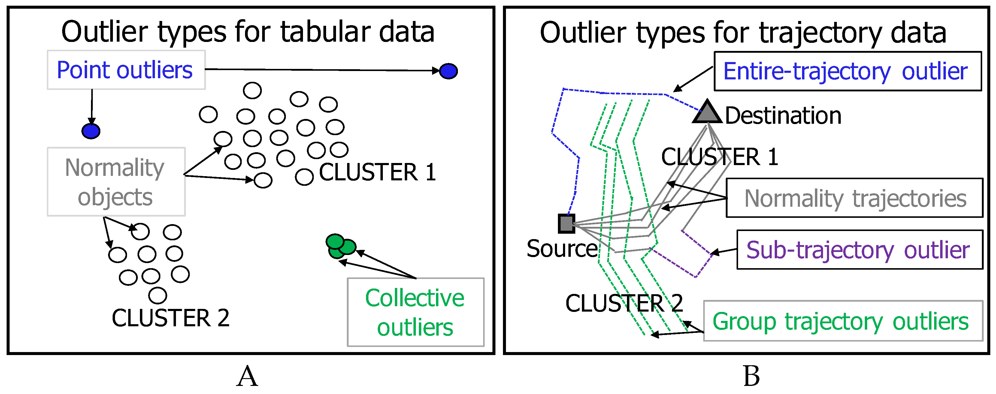
Figure 1. Outlier types. (A) tabular data: point and collective outliers; (B) trajectory data: sub-, entire-, and group-trajectory outliers.
Remotesensing 14 05394 g001
Figure 2. Typical outlier detection process for tabular (top) and trajectory data (bottom).
Remotesensing 14 05394 g002
Figure 3. Problems of different pre-processing methods. (Top left) Grid-based: both blue and red dash trajectories were represented by a series of cells which are visited for one time; hence, they were easier to be detected as outliers, while a red dash trajectory was actually a normality. (Top right) Sampling-based: two trajectories recorded on the same road but with different recording frequencies or different traveling speeds of the moving objects would lead to different sampling results shown as green points. (Bottom right) Partitioning-based: a noise or an outlier shown as the red triangle would produce different partitioning results.
Remotesensing 14 05394 g003
Figure 4. An example of how MiPo converts trajectory data (Bottom left, black rectangle box) to tabular data (Bottom right, red rectangle box). MiPo extracts two groups of features from trajectory data, namely the distance (Top, purple rectangle box) and point features (Bottom centre, green rectangle box) and merges them as the representation of the original trajectory.
Remotesensing 14 05394 g004
Figure 5. (Left) Normalities of three raw datasets with different source and destination points. (Right) Example of datasets with outliers. More information is reflected in Table 1.
Remotesensing 14 05394 g005
Figure 6. Models for different injected outlier types. (Left) Detour: a sub-trajectory was replaced with another sub-trajectory (red). (Middle) Perturbation: randomly selected points (red) were moved from their original places. (Right) Route-switching: two sub-trajectories (red) from two different trajectories were connected as an outlier trajectory.
Remotesensing 14 05394 g006
Figure 7. The outlier scores produced by M i P o + L O F (original) can be processed by NA to improve the results. NA(V) and NA(F) refer to setting NA’s parameter n _ n e i g h b o r to be varied or fixed.
Remotesensing 14 05394 g007
Figure 8. The effect of k for MiPo: distance between the source and destination matters.
Remotesensing 14 05394 g008
Figure 9. The effect of n _ n e i g h b o r for LOF: outlier types matter.
Remotesensing 14 05394 g009
Figure 10. Results when tuning both k for MiPo and n _ n e i g h b o r for LOF at the same time. Good results could be obtained by setting larger values for both k and n _ n e i g h b o r .
Remotesensing 14 05394 g010
Figure 11. Running time (s) of MiPo-, MiPo, MiPo+LOF, and baseline trajectory outlier detection methods varying the number of the trajectories n and the trajectory length m. The proposed MiPo was linear to n and m. Additionally, MiPo+LOF had much lower time complexity than accuracy-competitive baselines, such as IBAT.
Remotesensing 14 05394 g011
Figure 12. The illustration of MiPo-, MiPo, and MiPo+.
Remotesensing 14 05394 g012
Figure 13. Examples of the potential applications of MiPo with the AiSq5D dataset.
Remotesensing 14 05394 g013
Table 1. Datasets with organic outliers marked with asterisk and injected outliers.
No.DatasetSizeOutliers (%)Outlier TypeTrajectory Length
(max, avg, min)
1AiSq5D111555 (5%)Detour73, 49, 36
2AiSq10D1115112 (10%)Detour75, 50, 36
3AiSq5P111556 (5%)Perturb61, 49, 36
4AiSq10P1115109 (10%)Perturb61, 49, 36
5AiSq5DP111556 (5%)Detour + Perturb70, 49, 36
6AiSq10DP1115112 (10%)Detour + Perturb70, 49, 36
7StSt5M *19210 (5%)Manually labeled30, 27, 18
8StSt10M *20220 (10%)Manually labeled30, 27, 18
9StSt5R1919 (5%)Route-switching38, 27, 18
10StSt10R20018 (10%)Route-switching38, 27, 18
11UnCh5M *76338 (5%)Manually labeled30, 19, 8
12UnCh10M *80681 (10%)Manually labeled30, 19, 8
Table 2. AUC results of trajectory outlier detectors and proposed methods (the best per row is bolded).
DatasetMiPo+LOFIBATIBOATRLOFLSTMATDCTPBAELSTMRNPAT
Proposed[18][19][45][42][27][67][41][33]
AiSq5D1.001.000.980.850.750.900.840.76-
AiSq10D0.980.990.970.780.760.800.870.77-
AiSq5P1.000.980.990.670.700.900.870.70-
AiSq10P1.000.980.980.690.720.820.870.72-
AiSq5DP1.000.980.980.800.710.920.800.71-
AiSq10DP0.990.990.970.680.730.830.810.73-
StSt5R0.990.900.800.790.560.560.610.56-
StSt10R0.990.920.700.610.580.590.570.58-
StSt5M1.001.000.850.870.710.430.870.710.62
StSt10M0.990.990.740.820.620.240.870.620.60
UnCh5M0.970.850.690.950.850.840.920.850.77
UnCh10M0.980.920.730.850.850.670.890.850.81
AVG0.990.960.870.780.710.710.820.710.70
STD0.010.050.120.100.090.210.110.090.10
Media0.990.980.910.790.720.810.870.720.70
Table 3. AUC results of tabular outlier detectors using with MiPo (the best per row is in bold).
DatasetDOD+MOD+LOFODINNCKNNMCDIForestSVMPCASOGABVAECOPABODROD
[76][76][37][81][82][83][84][85][86][87][88][89][90][91][92]
AiSq5D0.970.980.990.810.601.000.960.950.940.960.260.970.931.000.91
AiSq10D0.960.970.980.800.550.990.920.930.860.890.300.840.890.990.88
AiSq5DP0.820.850.980.960.650.950.930.920.720.790.480.780.880.980.87
AiSq10DP0.860.890.970.900.520.950.890.890.710.800.330.770.860.980.88
AiSq5P0.760.770.970.990.670.930.940.930.630.890.350.870.900.980.90
AiSq10P0.750.770.970.970.660.920.930.920.630.860.440.830.900.980.89
StSt5R0.890.890.770.890.700.890.900.920.350.450.440.630.600.970.53
StSt10R0.870.860.850.880.520.880.870.890.290.360.360.660.430.920.46
StSt5M0.880.880.860.970.710.960.890.990.470.520.280.630.641.000.61
StSt10M0.880.880.820.870.620.930.920.970.580.620.420.720.700.960.61
UnCh5M0.950.960.940.660.490.960.950.950.950.940.120.940.950.940.93
UnCh10M0.950.950.800.640.530.960.970.970.940.960.100.930.960.960.93
AVG0.880.890.910.860.600.940.920.940.670.750.320.800.800.970.78
STD0.070.070.080.120.080.040.030.030.230.210.120.120.170.020.18
MEDIAN0.880.880.950.890.610.950.930.930.670.830.340.810.890.980.88
Table 4. Running time (s) of MiPo-, MiPo, MiPo+LOF, and baseline trajectory outlier detector.
(n, m)MiPo-MiPoMiPo+LOFIBATIBOATRapidLOFLSTMATDCTPBAELSTMAERNPAT
Proposed[18][19][45][42][27][67][41][33]
(100, 30)<0.010.150.150.790.580.013.540.061.123.02447.15
(100, 60)0.010.250.250.860.760.0211.090.091.329.66658.08
(100, 90)0.010.340.340.930.840.0418.040.151.2817.57800.2
(1000, 30)0.041.071.0916.3928.980.1340.073.57105.6137.262615.72
(1000, 60)0.071.941.9617.0434.440.2486.714.05114.9573.644062
(1000, 90)0.092.862.8817.5839.240.37158.254.91119.04127.035690.37
(10,000, 30)0.369.5210.89210.02315.432.06389.04319.3410,616.66346.1930,834.41
(10,000, 60)0.5918.1519.42220.48376.963.25720.84343.7210,576.89719.0251,515.42
(10,000, 90)0.7926.6927.97239.64423.234.581218.9377.9310,897.321326.2980,572.54
Publisher’s Note: MDPI stays neutral with regard to jurisdictional claims in published maps and institutional affiliations.