
A Novel Error Criterion of Fundamental Matrix Based on Principal Component Analysis


Abstract

1. Introduction
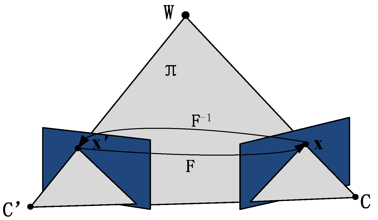
2. Computing FM
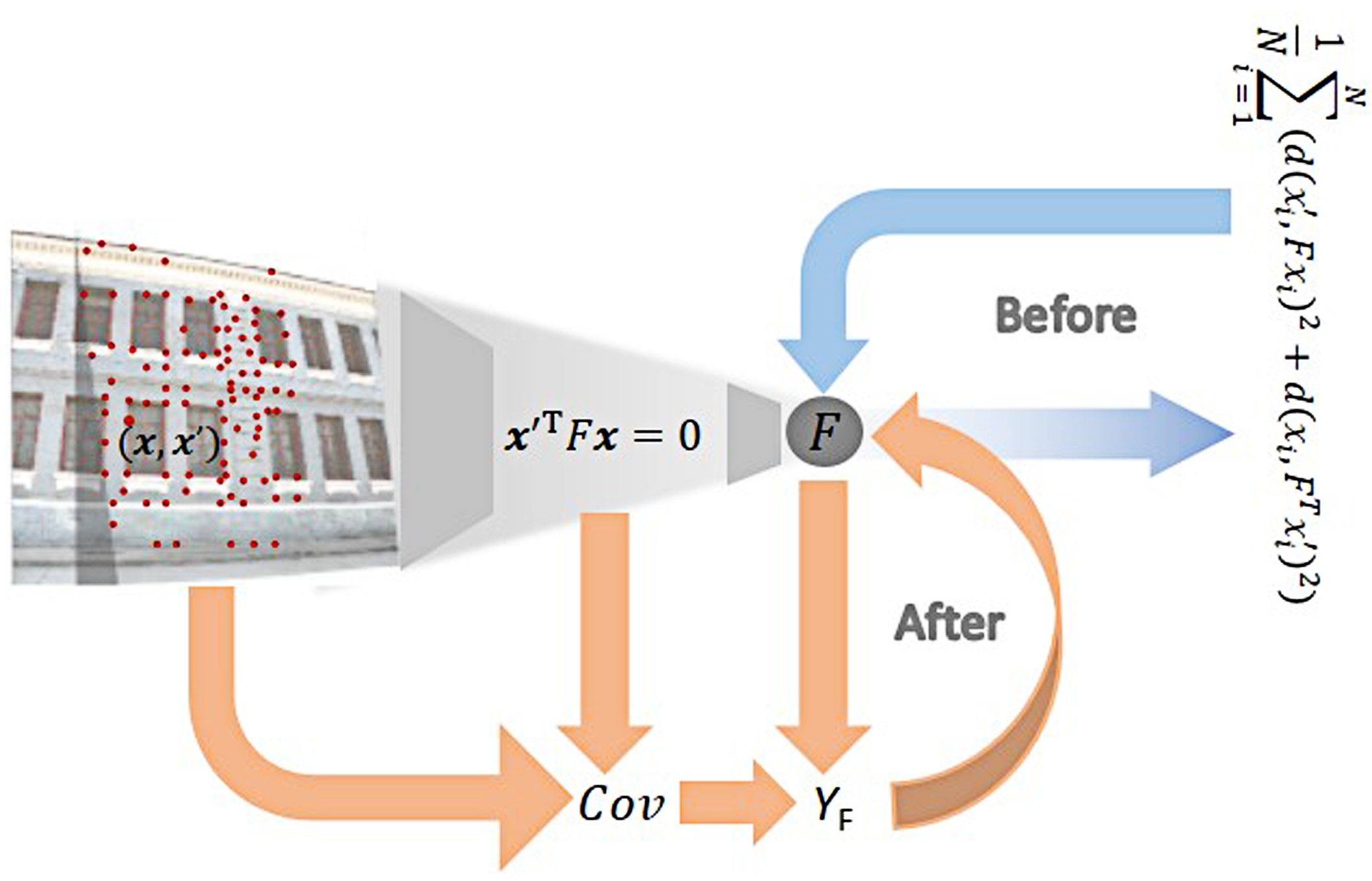
3. Quantization of FM Error
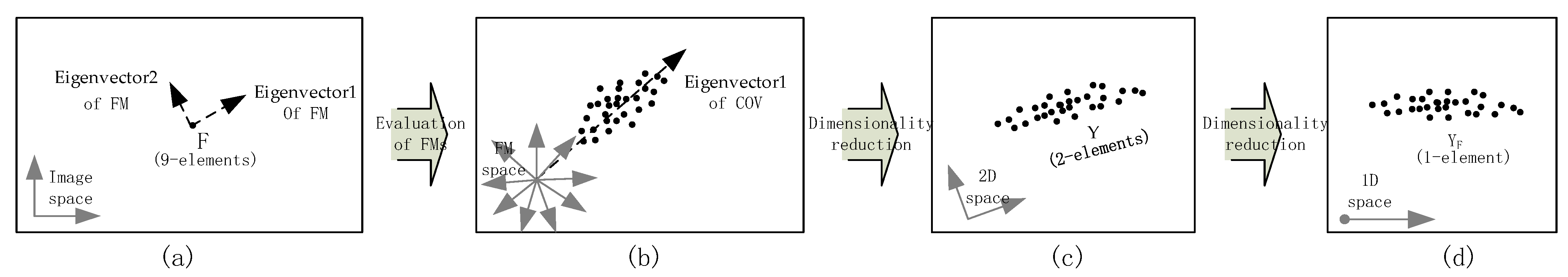
3.1. Covariance Matrix of FM
3.1.1. Matrix Differential Theory
- (1)
- The derivative of the constant matrix L is a zero matrix, i.e.,
- (2)
- The derivative of the inverse matrix is
- (3)
- The derivative of the matrix function product is
3.1.2. Covariance Matrix Derivation
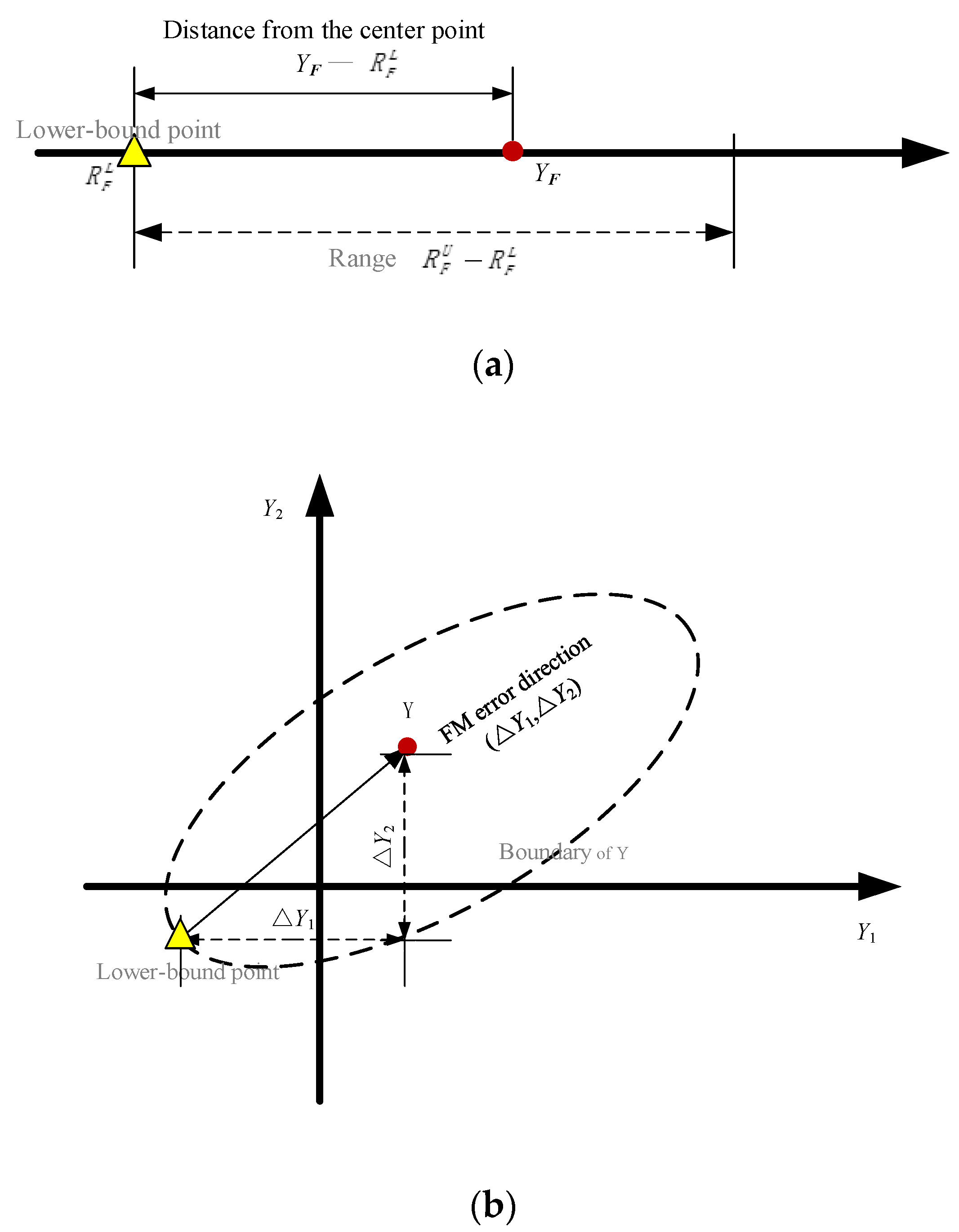
3.2. Scalar Function of FM Error
3.3. Review of the Proposed Method
| Algorithm 1. The calculated steps of FM error. |
|
4. Experiment
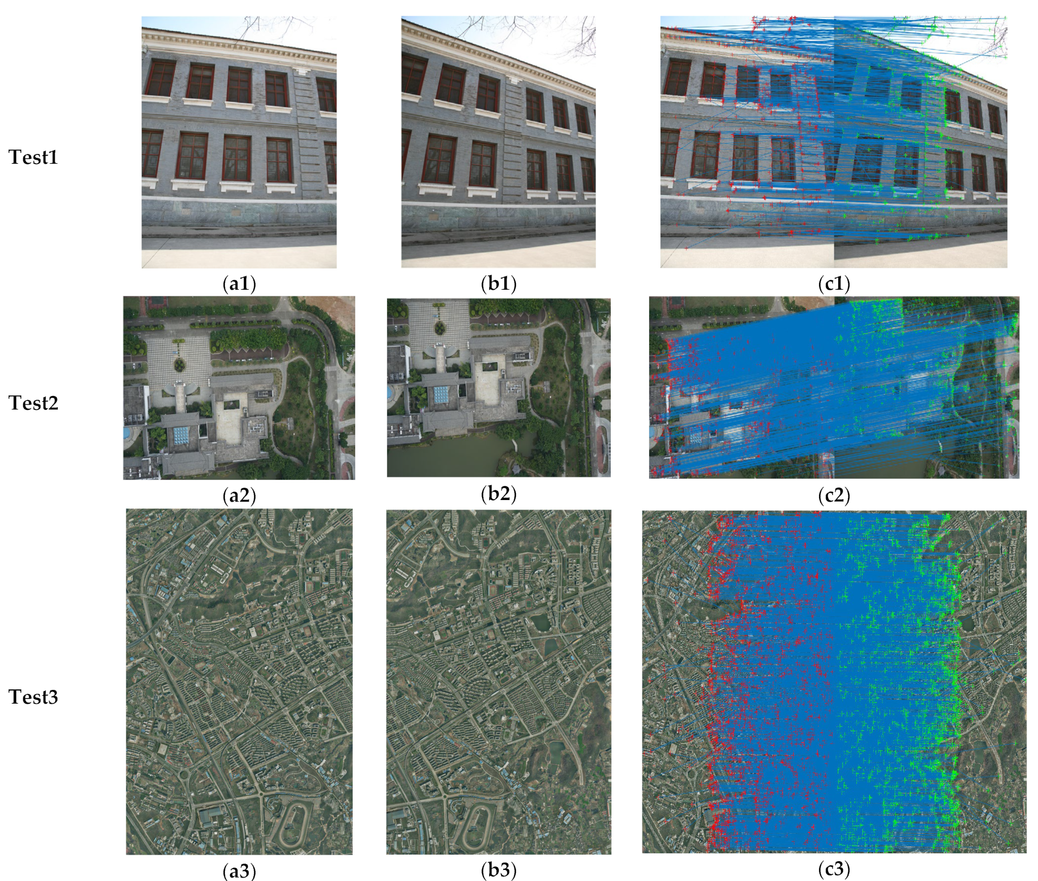
4.1. Data Source
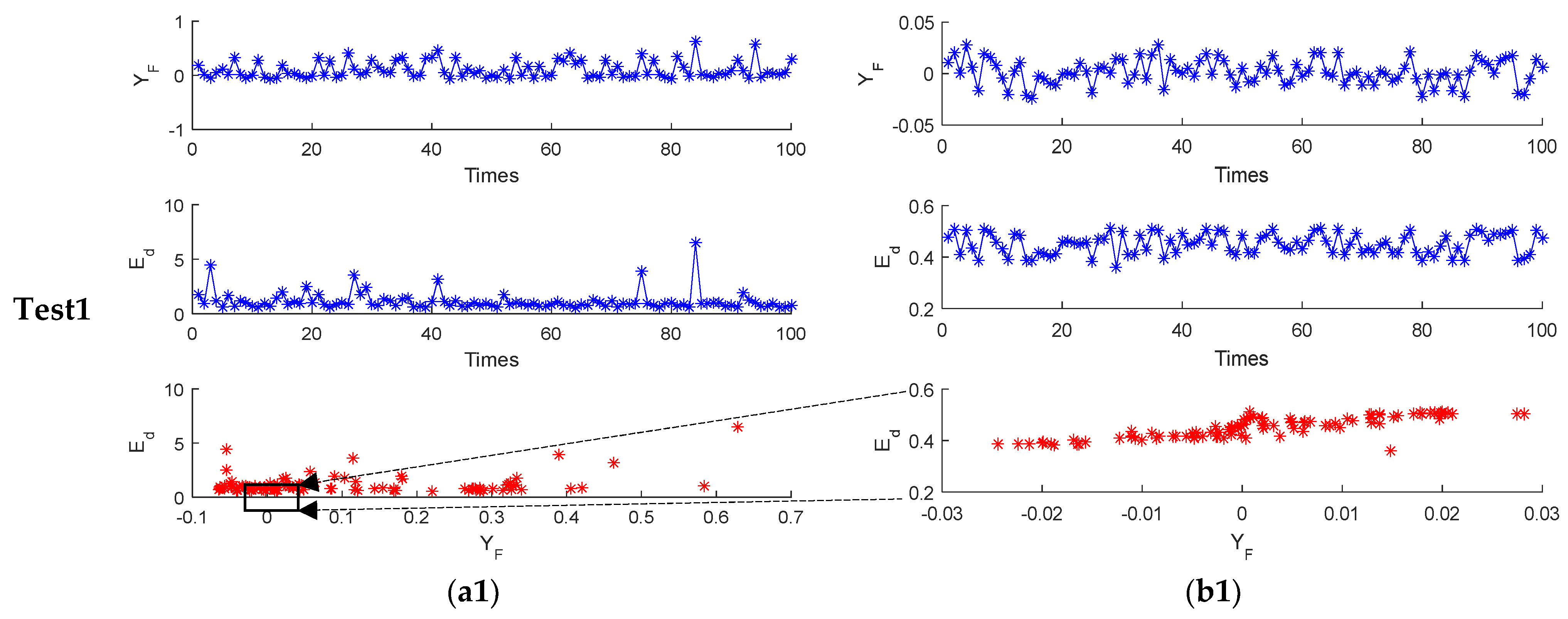
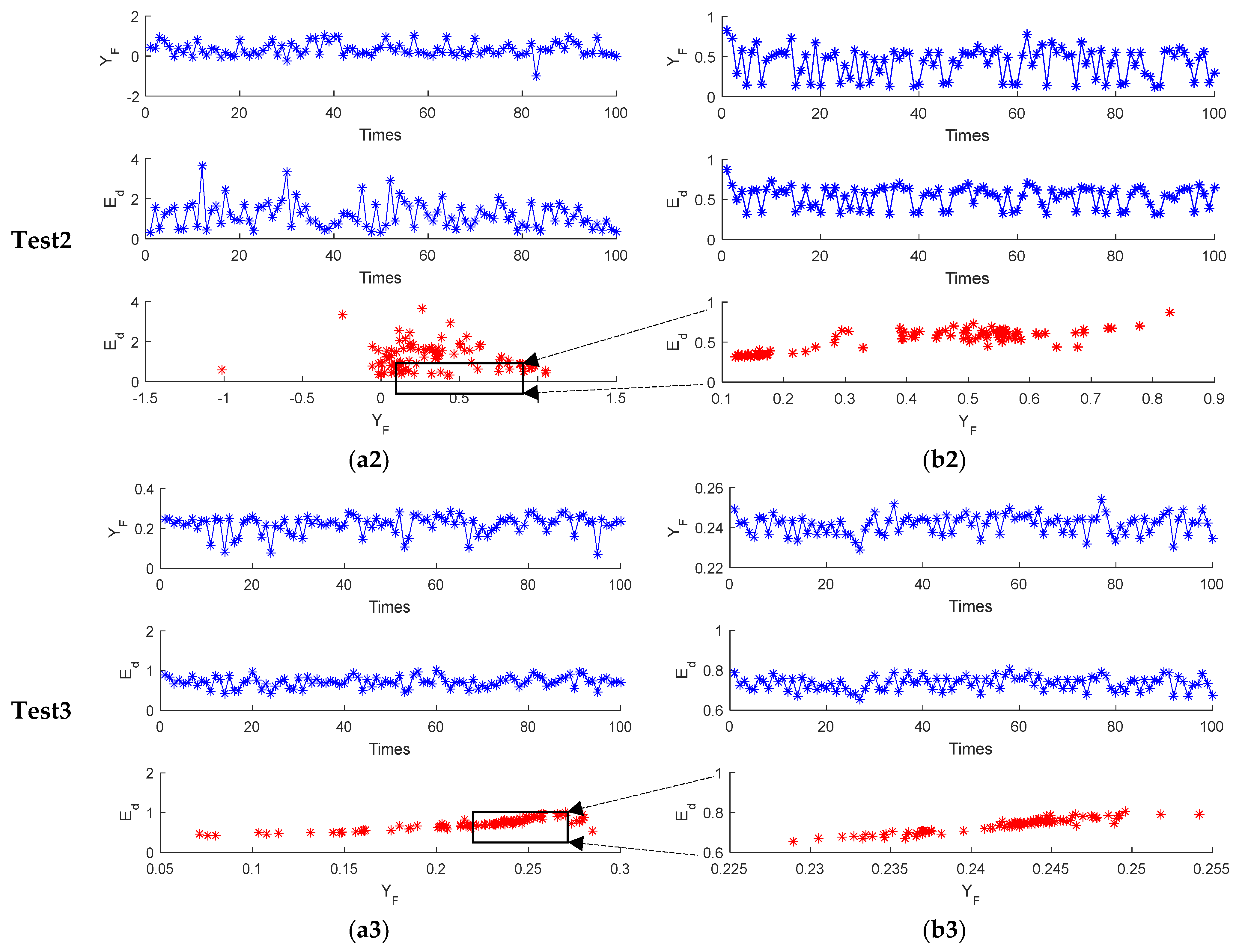
4.2. Correctness of Scalar Function
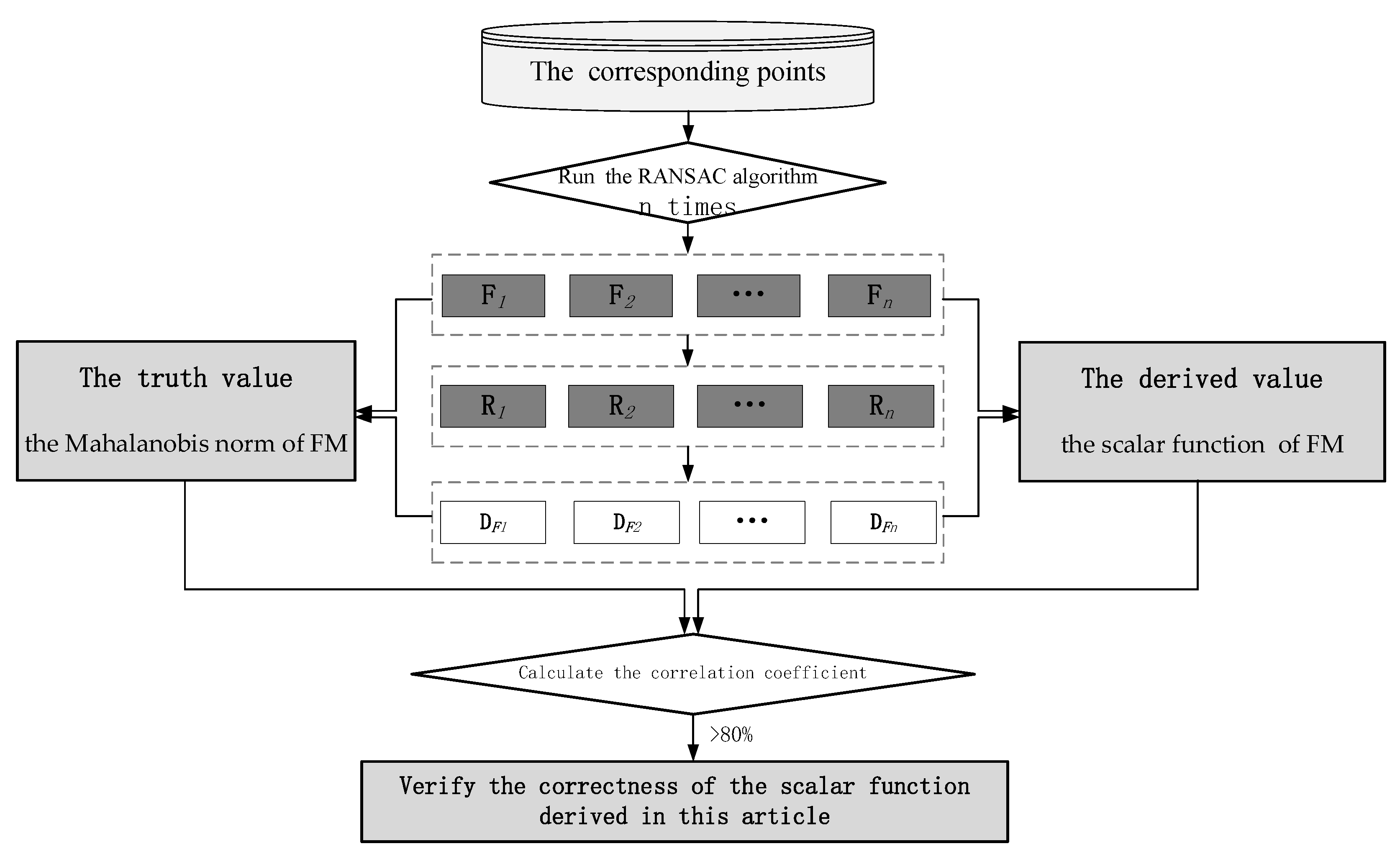
4.2.1. Experiment Process
- 1.
- The RANSAC algorithm is run n times to obtain n Ri sets of corresponding points after eliminating outliers, with which the covariance matrix DFi can then be calculated by Equation (20), where .
- 2.
- The Mahalanobis norm can be calculated following Equation (27), which is considered the truth value of FM error.
- 3.
- The scalar function YF can also be calculated using Equation (26), which is a measured value of FM error.
- 4.
- The correlation of the truth and measured errors can be calculated. When the correlation coefficient is large enough, the scalar function derived in this article is considered correct.
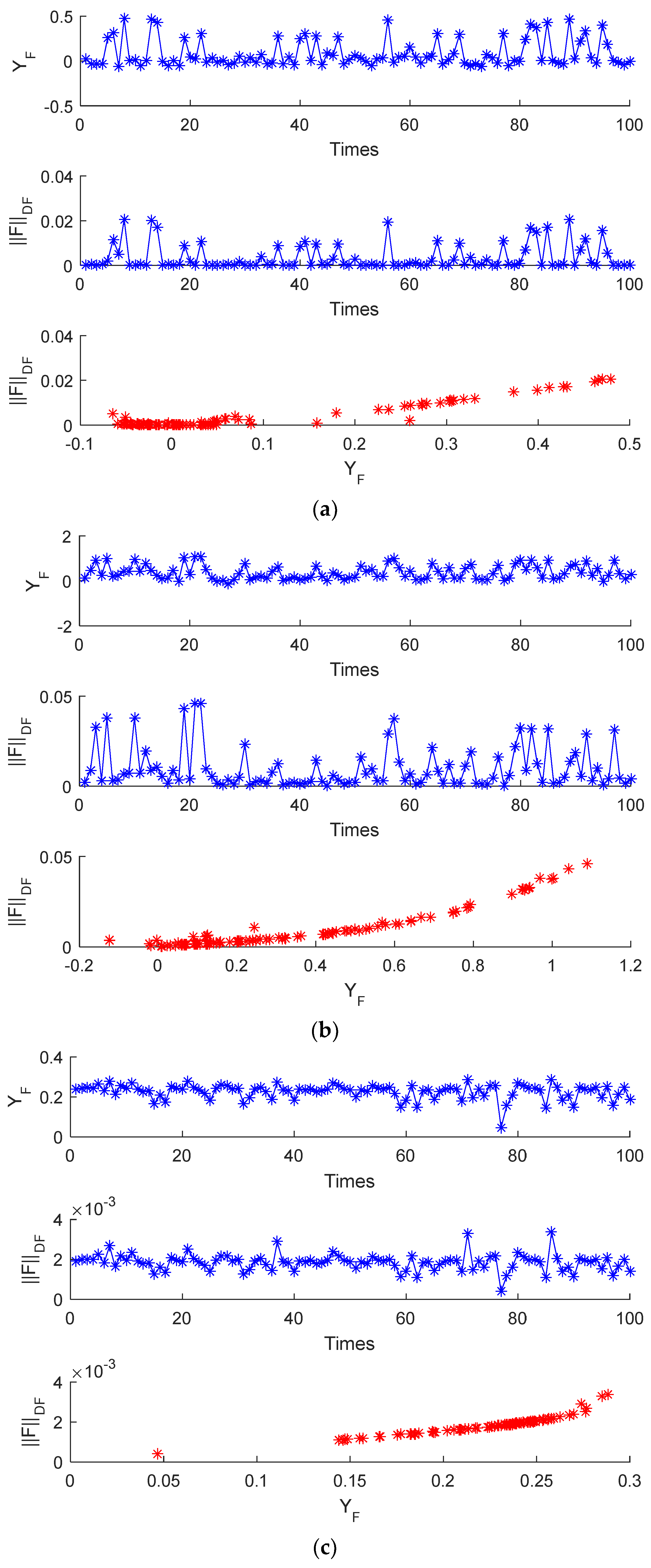
4.2.2. Experiment Result
4.3. Comparison with the Existing Method
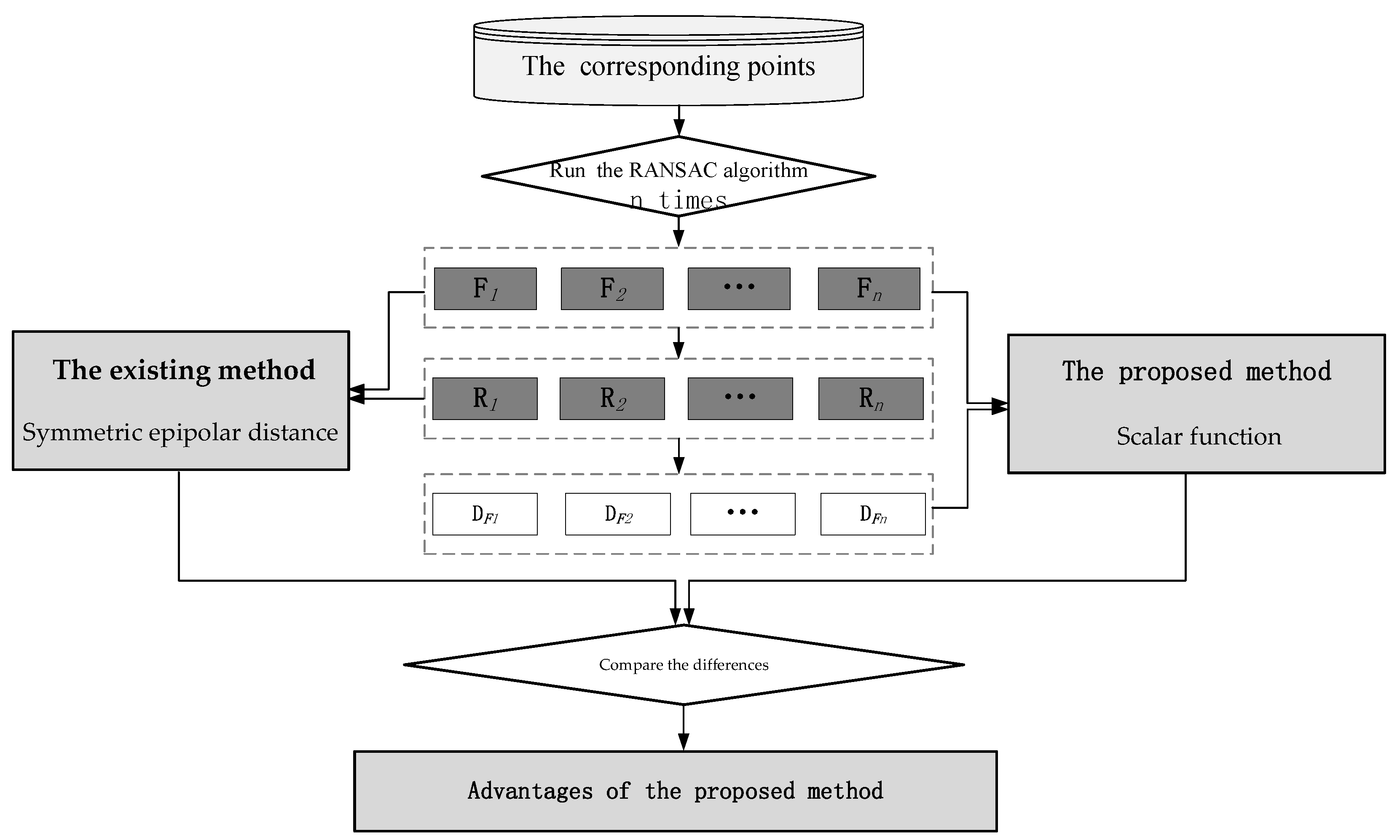
4.3.1. Experiment Process
- 1.
- The RANSAC algorithm is run n times to obtain n Ri sets of corresponding points after eliminating errors, with which the covariance matrix DFi can then be calculated by Equation (20), where .
- 2.
- The symmetric epipolar distance can be calculated following Equation (28), which is considered as the compared value of FM error.
- 3.
- The scalar function YF can be calculated using Equation (26), which is a measured value of FM error.
- 4.
- After the correlation of Steps 2 and 3 is calculated, the difference between the proposed method and the existing method can be analyzed.
4.3.2. Experiment Result
4.4. Application of This Method
5. Discussion
6. Conclusions
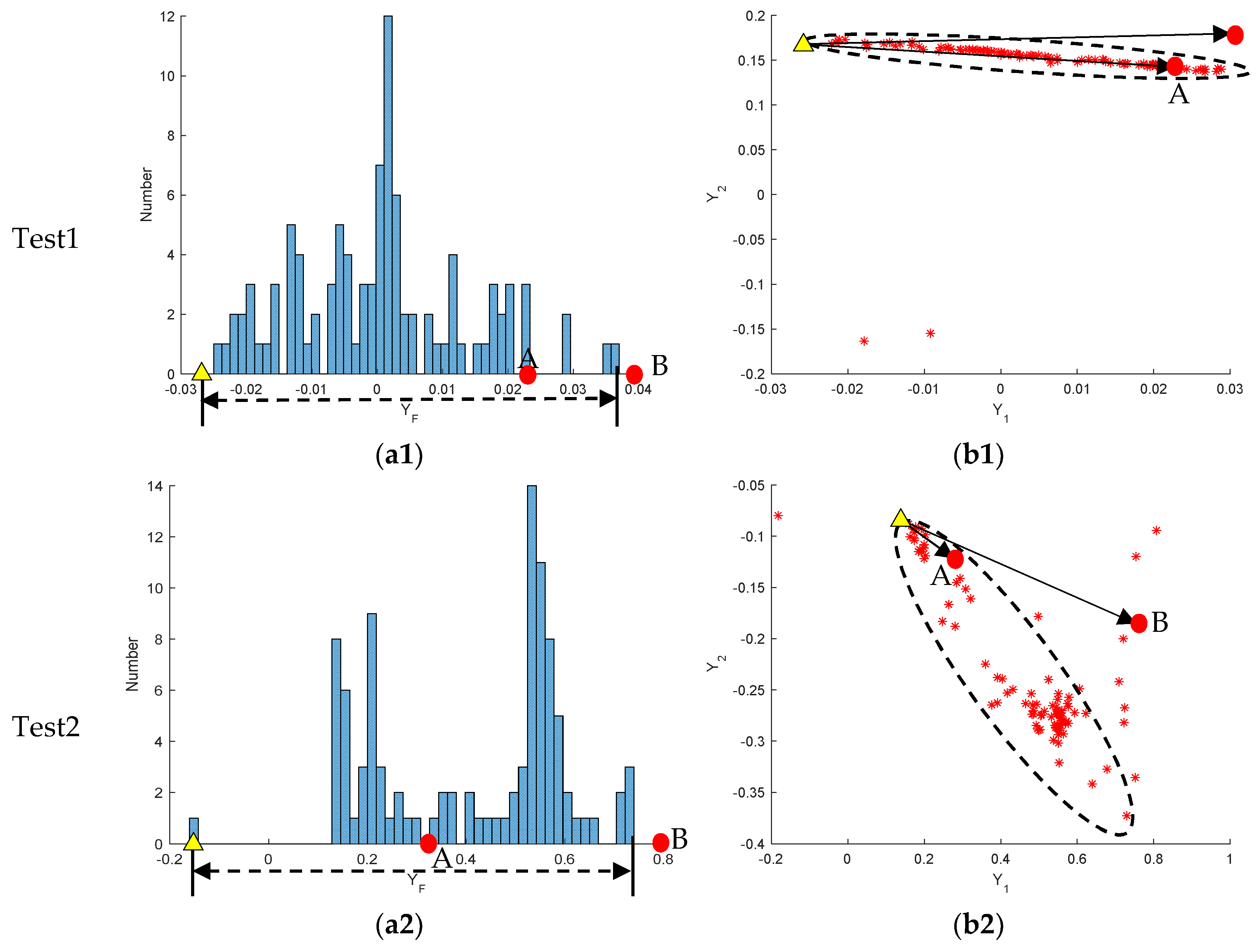
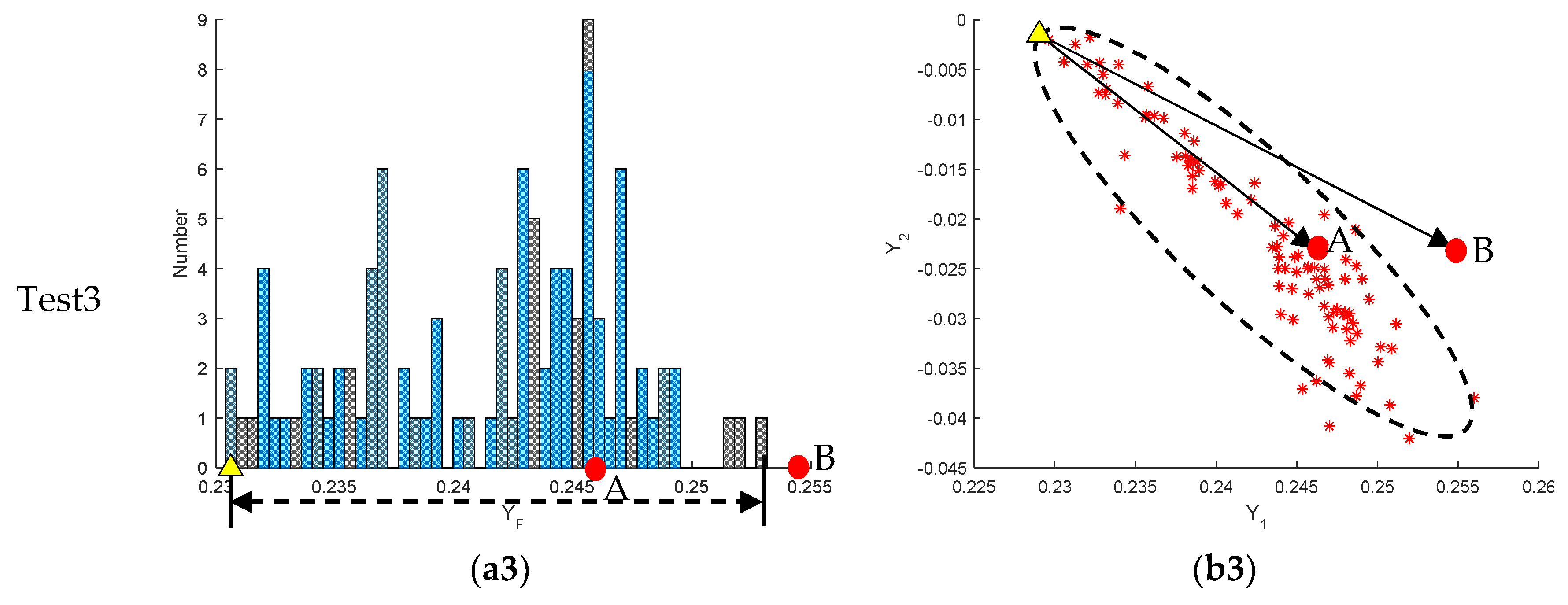
- Compute the covariance matrix using the known corresponding points extracted from two uncalibrated images.
- Following the PCA method, decompose the covariance matrix and then construct the vector Y and the scalar function YF.
- Count or calculate the boundary of Y and YF, and then calculate the ratio RF to estimate FM error. Here, the FM corresponding to is considered reasonable. When RF > 1, it is considered a low-quality FM.
Author Contributions
Funding
Data Availability Statement
Conflicts of Interest
References
- Rousseeuw, P.; Leroy, A. Robust Regression and Outlier Detection; John Wiley & Sons: New York, NY, USA, 1987; pp. 216–245. [Google Scholar]
- Fischler, M.A.; Bolles, R.C. Random sample consensus: A paradigm for model fitting with applications to image analysis and automated cartography. In Readings in Computer Vision; Morgan Kaufmann: Burlington, MA, USA, 1987; pp. 726–740. [Google Scholar] [CrossRef]
- Faugeras, O.D.; Luong, Q.T.; Maybank, S.J. Camera self-calibration: Theory and experiments. Proc. ECCV 1992, 588, 321–334. [Google Scholar] [CrossRef]
- Hartley, R.I.; Gupta, R.K.; Chang, T. Stereo from uncalibrated cameras. In Proceedings of the 1992 IEEE Computer Society Conference on Computer Vision and Pattern Recognition, Champaign, IL, USA, 15–18 July 1992. [Google Scholar] [CrossRef]
- Hartley, R.I. Estimation of relative camera positions for uncalibrated cameras. In Proceedings of the Second European Conference on Computer Vision, Santa Margherita Ligure, Italy, 19–22 May 1992; pp. 579–587. [Google Scholar] [CrossRef]
- Longuet-Higgins, H.L. A computer algorithm for reconstructing a scene from two projections. In Readings in Computer Vision; Morgan Kaufmann: San Franciso, CA, USA, 1987; pp. 61–62. [Google Scholar] [CrossRef]
- Hartley, R.I. Euclidean reconstruction from uncalibrated views. In Proceedings of the Second Joint European—US Workshop on Applications of Invariance in Computer Vision, Azores, Portugal, 9–14 October 1993; Volume 825, pp. 237–256. [Google Scholar] [CrossRef]
- Hartley, R.; Zisserman, A.; Faugeras, O. Multiple View Geometry in Computer Vision, 2nd ed.; Cambridge University Press: Cambridge, UK, 2003; pp. 90–99, 178–190, 195–202. [Google Scholar]
- Tian, Z.; Li, B.C. Optimize preview model parameters evaluation of RANSAC. Appl. Mech. Mater. 2012, 687, 3984–3987. [Google Scholar] [CrossRef]
- Torr, P.; Murray, D.W. The development and comparison of robust methods for estimating the fundamental matrix. Int. J. Comput. Vis. 1997, 24, 271–300. [Google Scholar] [CrossRef]
- Armangué, X.; Salvi, J. Overall view regarding fundamental matrix estimation. Image Vis. Comput. 2003, 21, 205–220. [Google Scholar] [CrossRef]
- Yan, K.; Liu, E.H.; Zhao, R.J. A fast and robust method for fundamental matrix estimation. Opt. Precis. Eng. 2018, 26, 1–10. [Google Scholar] [CrossRef]
- Chen, F.X.; Wang, R.S. Fast RANSAC with preview model parameters evaluation. J. Softw. 2005, 16, 1431–1437. [Google Scholar] [CrossRef]
- Wang, G.; Sun, X.L.; Shang, Y.; Wang, Z.; Shi, Z.C.; Yu, Q.F. Two-view geometry estimation using RANSAC with locality preserving constraint. IEEE Access 2020, 8, 726–7279. [Google Scholar] [CrossRef]
- Yang, M.; Liu, Y.; You, Z. Estimating the fundamental matrix based on least absolute deviation. Neurocomputing 2011, 74, 3638–3645. [Google Scholar] [CrossRef]
- Torr, P.; Zisserman, A. MLESAC: A new robust estimator with application to estimating image geometry. Comput. Vis. Image Underst. 2000, 78, 138–156. [Google Scholar] [CrossRef]
- Torr, P.H.S. Bayesian model estimation and selection for epipolar geometry and generic manifold fitting. Int. J. Comput. Vis. 2002, 50, 35–61. [Google Scholar] [CrossRef]
- Wei, R.Y.; Wang, J.F. FSASAC: Random sample consensus based on data filter and simulated annealing. IEEE Access 2021, 9, 164935–164948. [Google Scholar] [CrossRef]
- Carro, A.I.; Morros, J.R. Promeds: An adaptive robust fundamental matrix estimation approach. In Proceedings of the 2012 3DTV-Conference: The True Vision—Capture, Transmission and Display of 3D Video (3DTV-CON), Zurich, Switzerland, 15–17 October 2012. [Google Scholar] [CrossRef]
- Vinod Kumar, S.; Arnab, M. Random sample consensus in decentralized kalman filter. Eur. J. Control. 2022, 65, 100617. [Google Scholar] [CrossRef]
- Shao, C.; Zhang, C.; Fang, Z.; Yang, G. A deep learning-based semantic filter for RANSAC-based fundamental matrix calculation and the ORB-SLAM system. IEEE Access 2019, 8, 3212–3223. [Google Scholar] [CrossRef]
- Fathy, M.E.; Hussein, A.S.; Tolba, M.F. Fundamental matrix estimation: A study of error criteria. Pattern Recognit. Lett. 2011, 32, 383–391. [Google Scholar] [CrossRef]
- Li, X.; Yuan, X. Fundamental matrix computing based on 3D metrical distance. Algorithms 2021, 14, 89. [Google Scholar] [CrossRef]
- Zhou, F.; Zhong, C.; Zheng, Q. Method for fundamental matrix estimation combined with feature lines. Neurocomputing 2015, 160, 300–307. [Google Scholar] [CrossRef]
- Yan, K.; Zhao, R.J.; Liu, E.H.; Ma, Y.B. A robust fundamental matrix estimation method based on epipolar geometric error criterion. IEEE Access 2019, 7, 147523–147533. [Google Scholar] [CrossRef]
- Liang, W.; Ju, G. A Global fundamental matrix estimation method of planar motion based on inlier updating. Sensors 2022, 22, 4624. [Google Scholar] [CrossRef]
- Yang, R.; Zhang, J.; Li, B. Estimating the fundamental matrix based on the end-to-end convolutional network. Appl. Intell. 2022, 52, 15517–15528. [Google Scholar] [CrossRef]
- Zhang, Z. Determining the epipolar geometry and its uncertainty: A review. Int. J. Comput. Vis. 1998, 27, 161–198. [Google Scholar] [CrossRef]
- Faugeras, O.; Zhang, Z.Y.; Zeller, C.; Csurka, G. Characterizing the uncertainty of the fundamental matrix. Comput. Vis. Image Underst. 2006, 68, 18–36. [Google Scholar] [CrossRef]
- Sur, F.; Noury, N.; Berger, M.O. Computing the uncertainty of the 8 point algorithm for fundamental matrix estimation. In Proceedings of the 19th British Machine Vision Conference—BMVC, Leeds, UK, 1–4 September 2008. [Google Scholar] [CrossRef]
- Raguram, R.; Frahm, J.M.; Pollefeys, M. Exploiting uncertainty in random sample consensus. In Proceedings of the 2009 IEEE 12th International Conference on Computer Vision, Kyoto, Japan, 29 September–2 October 2009; pp. 2074–2081. [Google Scholar] [CrossRef]
- Bian, Y.X. Research on the Uncertainty of 3D Point Cloud Reconstruction Based on Image Sequences. Ph.D. Thesis, Nanjing Normal University, Nanjing, China, 2015. [Google Scholar]
- Jolliffe, I.T.; Cadima, J. Principal component analysis: A review and recent developments. Philos. Trans. A Math. Phys. Eng. 2016, 374, 20150202. [Google Scholar] [CrossRef] [PubMed]
- Grtler, J.; Spinner, T.; Streeb, D. Uncertainty-aware principal component analysis. IEEE Trans. Vis. Comput. Graph. 2020, 26, 822–831. [Google Scholar] [CrossRef] [PubMed]
- Shi, C.Y. Guide to the Expression of Uncertainty in Measurement; China Metrology Publishing House: Beijing, China, 2000; pp. 9–10. [Google Scholar]
- Zhang, X.D. Matrix Analysis and Applications; Qinghua University Press: Beijing, China, 2004; pp. 43–53. [Google Scholar]


Publisher’s Note: MDPI stays neutral with regard to jurisdictional claims in published maps and institutional affiliations. |
© 2022 by the authors. Licensee MDPI, Basel, Switzerland. This article is an open access article distributed under the terms and conditions of the Creative Commons Attribution (CC BY) license (https://creativecommons.org/licenses/by/4.0/).
Share and Cite
Bian, Y.; Fang, S.; Zhou, Y.; Wu, X.; Zhen, Y.; Chu, Y. A Novel Error Criterion of Fundamental Matrix Based on Principal Component Analysis. Remote Sens. 2022, 14, 5341. https://doi.org/10.3390/rs14215341
Bian Y, Fang S, Zhou Y, Wu X, Zhen Y, Chu Y. A Novel Error Criterion of Fundamental Matrix Based on Principal Component Analysis. Remote Sensing. 2022; 14(21):5341. https://doi.org/10.3390/rs14215341
Chicago/Turabian StyleBian, Yuxia, Shuhong Fang, Ye Zhou, Xiaojuan Wu, Yan Zhen, and Yongbin Chu. 2022. "A Novel Error Criterion of Fundamental Matrix Based on Principal Component Analysis" Remote Sensing 14, no. 21: 5341. https://doi.org/10.3390/rs14215341
APA StyleBian, Y., Fang, S., Zhou, Y., Wu, X., Zhen, Y., & Chu, Y. (2022). A Novel Error Criterion of Fundamental Matrix Based on Principal Component Analysis. Remote Sensing, 14(21), 5341. https://doi.org/10.3390/rs14215341