Abstract
This study applies Gravity Recovery and Climate Experiment (GRACE) data and the WaterGAP (Water Global Analysis and Prognosis) Global Hydrology Model (WGHM) to investigate the influence of the Bui reservoir operation on water storage variation within the Volta River Basin (VRB). Variation in groundwater storage anomalies (GWSA) was estimated by combining GRACE-derived terrestrial water storage anomalies (TWSA), radar altimetry records, imagery-derived reservoir (Lake Volta and Bui) surface water storage anomalies (SWSA), and Global Land Data Assimilation System (GLDAS)-simulated soil moisture storage anomalies (SMSA) from 2002 to 2016. Results showed that TWSA increased (1.30 ± 0.23 cm/year) and decreased (−0.82 ± 0.27 cm/year) during 2002–2011 and 2011–2016, respectively, within VRB, matching previous TWSA investigations in this area. It revealed that the multi-year averages of monthly GRACE-derived TWSA changes in 2011–2016 displayed an overall increasing trend, indicating storage increase in regional hydrology; while the Lake Volta water storage changes decreased. The GRACE-minus-WGHM residuals display an increasing trend in VRB water storage during the Bui reservoir impoundment during 2011–2016. The observed trend compares well with the estimated Bui reservoir SWSA, indicating that GRACE solutions can retrieve the true amplitude of large mass changes happening in a concentrated area, though Bui reservoir is much smaller than the resolution of GRACE global solutions. It also revealed that GWSA were almost stable from 2002 to 2006, before increasing and decreasing during 2006–2011 and 2012–2016 with rates of 2.67 ± 0.34 cm/year and −1.80 ± 0.32 cm/year, respectively. The observed trends in the GRACE-derived TWSA and GWSA changes are generally attributed to the hydro-meteorological conditions. This study shows that the effects of strong El-Niño Southern Oscillation events on the GWSA interannual variability within the VRB is short-term, with a lag of 6 months. This study specifically showed that the Bui reservoir operation significantly affects the TWSA changes and provides knowledge on groundwater storage changes within the VRB.
1. Introduction
The Volta River Basin (VRB), covering almost 400,000 km2, approximately 28% of Africa’s continental West Coast, is one of the main river networks in Africa. The basin stretches over six different countries: Ghana, Benin, Ivory Coast, Togo, Burkina Faso, and Mali. Water and environmental resources of the VRB have undergone extreme stress due to the complex configuration of geographical and social aspects, as well as incessant stress of climate change [1,2]. Therefore, the basin-living people are extremely sensitive to temporal and spatial precipitation and climate change. In addition, water resources scarcity will be further aggravated due to deforestation, high land degradation rate coupled with climate change, and high population growth [3,4,5]. In 2007, to mitigate the future danger for the well-being of their populations, administrations of the six aforementioned countries established some action plans under the responsibility of the Volta Basin Authority, built on fundamentals of integrated water resources management [6]. To execute these action plans, scientific investigations on the recent trends and future predictions of water availability in the basin are required to help the decision makers and advisors.
Recurrent flooding events and the increasing needs for freshwater and power supplies have led to the development of major new engineering projects (e.g., dams) across the VRB. One of world largest man-made lakes (Lake Volta) is located in the VRB. Lake Volta is presently the main lake in the VRB, and is controlled by the Akosombo dam, which has been in operation since 1965. Besides Akosombo dam, a new important dam, called Bui dam was constructed from 2009 to 2010, and its reservoir impoundment started in 2011. The Bui dam was commissioned for use in 2013. In the VRB, especially in the Afram Plains area (with a total land area of approximately 3095 km2), annual increase in domestic water needs of approximately 2.5% due to the projected annual increase in population would induce an increase in groundwater withdrawal rates from 12,800 m3/day in 2015 to approximately 30,400 m3/day by 2050 [7]. Indeed, along the tropics and in many parts of Sub-Saharan Africa, groundwater is the main source for freshwater and for irrigated agriculture [8]. Groundwater inevitably becomes the water source in dry areas far from streams and reservoirs or to alleviate water shortage during droughts. In order to achieve the Sustainable Development Goals, ensuring the development and the adjustment to climate changes throughout Africa, groundwater resources will be increasingly used [9,10]. In this case, it is imperative to investigate groundwater storage variation, examining the repercussions of human activities (e.g., construction of dams) and the impacts of climate changes.
Across West Africa, the roles of climatic change have been largely reported, whether it is at regional or basin level [11,12,13,14,15,16,17,18,19,20]. It is shown that rainfall patterns and hydro-meteorological conditions are influenced by the large-scale ocean-land-atmospheric interchanges and global climate teleconnections (e.g., El-Niño Southern Oscillation (ENSO), Atlantic Multi-decadal Oscillation (AMO)). Climate change causes severe weather episodes. The major findings of previous studies on terrestrial water storage in West Africa (including the VRB) [3,18,21,22,23,24,25,26] largely agree on the statistically significant changes in terrestrial water storage due to anthropogenic and natural causes. Terrestrial water storage is the vertical integration of surface water storage (e.g., reservoirs, lakes, rivers), soil moisture storage, groundwater storage, snow, and ice storage, as well as canopy storage. These water components might react differently to climate change, as rainfall is the main input for terrestrial water storage. Long periods of drought and flood directly affect groundwater availability and dependency. However, none of the above studies have addressed groundwater storage variation, or the impact of climate teleconnections and human activities on groundwater storage variation in the VRB.
Indeed, the most recent methods to monitor groundwater storage changes were based on a network of accurately located and designed observation wells, which monitor changes in groundwater levels over a long-term period [7,27]. However, according to Famiglietti et al. [28], remote sensing can supply large-scale data in water stock variation, which are steady across national boundaries. Nevertheless, so far in the VRB, due to the lack of basin-wide in situ data, there is no significant investigation of groundwater storage changes at basin scale. The present study aims to investigate changes in groundwater stocks, including the impact of human activities (e.g., construction of dams) and climate teleconnections influences in the VRB, using large-scale remotely sensed data from satellite gravimetry such as the Gravity Recovery and Climate Experiment (GRACE).
GRACE provides monthly, vertically integrated estimations of terrestrial water storage anomalies (TWSA) related to a specific baseline or long-term average at a spatial resolution > 100,000 km2. As indicated above, groundwater is one component of terrestrial water storage. Therefore, groundwater storage can be isolated from the GRACE terrestrial water storage estimates by removing independent estimates of all other water components (e.g., surface water storage, soil moisture storage). An increase in the application of remote sensing and global models of groundwater investigations can be observed across the world, especially in areas where ground-based data are unavailable at large scale, such as the Volta River Basin. Global land surface models (LSMs) and global hydrologic models (GHMs) are the two main global models that provide independent estimates of water budget components. The LSMs are mostly established to design the limit condition for climate standards including water and energy conservation. Most of LSMs, such as Global Land Data Assimilation System (GLDAS), do not contain information about human activities and broadly limit their contents to soil moisture and snow. Bonsor et al. [29] investigated the seasonal and decadal groundwater changes in African sedimentary aquifers (not including the VRB), by combining GRACE products and LSM outputs. Their work revealed an inconsistency between the GRACE-LSMs driven results and in situ data of groundwater recharge from different basins. Consequently, Bonsor et al. [29] highlighted the need for more in situ data from wells to further improve the LSMs outputs. The GHMs, based on water balance, were basically established to assess water shortage. While most GHMs do not introduce energy balance, all the models mostly contain surface water, soil moisture, and groundwater. In contrast to LSMs, the GHMs mostly include human activities, such as water withdraw, return flow from surface water or groundwater withdrawal, and reservoir storage. In many parts of the world (such as major U.S. aquifers, North China Plain, Tigris-Euphrates Basin, Three Gorges Reservoir, Northwest India, etc.), the GHMs have been applied to investigate human activity impacts on water storage changes [30,31,32,33].
This study, therefore, aims to (i) investigate the influences of the Bui reservoir operation and climate changes on the TWSA changes within the VRB; (ii) estimate the groundwater storage anomalies (GWSA) changes; (iii) quantify the contributions of water components into the basin’s TWSA changes and understand their temporal dynamics. The GWSA analysis was restricted to the basin’s fractured land, which contains the Lake Volta and Bui reservoir (Figure 1).
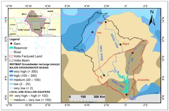
Figure 1.
Study area showing the Volta River Basin and its river system (Black Volta, White Volta, and Oti River). The shaded region in the inset map is the extent of the Volta River Basin.
2. Study Area and Data Used Materials
2.1. The Volta River Basin
The Volta River Basin is one of the largest basins in sub-Saharan Africa, extending approximately between latitudes 5°30’N–14°30’N and longitudes 5°30’W–2°00’E. It spreads out across at least four climatic regions, oriented from lowland rainforest in the south, to the semi-arid Sahel-Sudan desert in the north [34]. The VRB is characterized by sedimentary aquifers, which are classified between the fractured zone and a mélange of intergranular and fractured land. The Volta Fractured Land, which is defined by the red line (Figure 1), is the main fractured land within the VRB, and therefore, offers good conditions for groundwater storage under the influences of extreme wet events [29,35]. The basin’s climate is generally characterized by two types of rainy seasons: unimodal and bimodal, which are mainly induced by the movement of the Inter-Tropical Convergence Zone (ITCZ) [34,36]. The basin’s hydrological network is divided into three main sub-catchments, namely the Nakambé and Mouhoun, which feed the White Volta and Black Volta rivers, respectively, and the Oti River. The Volta River generally flows south across Ghana and discharges into the Gulf of Guinea. The flows of the rivers are relatively managed by dams to support power and water resources. Groundwater aquifer depths are shallow in most parts of the basin, while a significant groundwater aquifer is present in the upper Volta basin (north-western). The information about the aquifer systems and their recharge properties were obtained from the World-wide Hydrogeological Mapping and Assessment Program (https://www.whymap.org/whymap/EN/Home/whymap_node.html, accessed on 10 January 2021) website. The map ‘‘Groundwater resources and recharge’’ gives knowledges on the types and properties of the global groundwater aquifer system. It should be noted that the GWSA changes estimation in this study will focus on the Volta Fractured Land area, which contains Lake Volta and Bui reservoir.
2.2. GRACE Data
Launched in March 2002, the GRACE satellite mission has improved the applications of remotely sensed data in a wide range of hydrological investigations. The GRACE twin satellites were designed to yield data on spatiotemporal variations in the Earth’s gravity field, which mainly include storage changes in surface water, soil moisture and groundwater. Therefore, vertically integrated estimates of TWSA related to a specific baseline or long-term average can be derived from GRACE products.
Monthly GRACE and GRACE-Follow Release-06 level-2 GSM products, provided by the Center for Space Research of the University of Texas at Austin, were used to estimate TWSA changes within the VRB relative to the 2004–2009 baseline. The GRACE products, expressed as spherical harmonic coefficients and up to degree/order 60, constitute the hydrological and geophysical signals over land, as oceanic and atmospheric mass variations have been separated. In this study, GRACE Matlab Toolbox (GRAMAT) (https://github.com/fengweiigg/GRACE_Matlab_Toolbox, accessed on 10 January 2021) developed by Feng et al. [37], was used to estimate TWSA.
2.3. TWSA from WGHM
The WaterGAP (Water Global Analysis and Prognosis) Global Hydrology Model (WGHM) reproduces day-to-day water flows and storages of the hydrological cycle globally with a spatial resolution of 0.5 degree. It has been implemented in many areas (e.g., Three Gorges Reservoir, North China Plain, Tigris-Euphrates Basin) to study human activity impacts on water storage changes [30,31,32,33]. The WGHM has been updated to version 2.2d, providing monthly output of terrestrial water storage changes, as well as all water resource components, including surface water storage (e.g., rivers, wetlands, lakes, and reservoirs) and soil moisture storage [38,39]. The WGHM combines exhaustive information on attributes, extent and location of lakes, reservoirs, and wetlands to simulate surface water changes. However, the global database of lakes and wetlands used by the WGHM does not include the Bui Reservoir [40]. Therefore, monthly WGHM-derived TWSAs relative to the 2004–2009 baseline were used in this study to investigate the influence of the Bui reservoir implementation on changes in TWSA within the VRB. The TWSA from WGHM were subtracted from the GRACE-estimated TWSA, before being compared with the water storage changes of both Lake Volta and Bui reservoir. It is worth recalling that the WGHM-derived TWSA were filtered in the same way as GRACE data before subtraction from the GRACE-estimated TWSA.
2.4. SMSA from GLDAS
Soil moisture is one of the storage changes in the water cycle, and its reliable estimation is crucial for an accurate segregation of the groundwater changes. In this case, the soil moisture storage changes used in this study were obtained by averaging the soil moisture storages from three types of GLDAS outputs (version 2.1), i.e., NOAH, CLM, and VIC. By integrating relevant terrestrial and satellite observations and applying a data assimilation approach, the global land surface model, GLDAS, can simulate optimal land water and energy fluxes. The GLDAS dataset was provided by Goddard Earth Sciences Data and Information Services Center, Greenbelt, Maryland, USA (https://disc.gsfc.nasa.gov/datasets?keywords=GLDAS, accessed on 10 January 2021).
2.5. Precipitation Data, Climate Indices and Drought Index
The 0.5° × 0.5° global grids of monthly estimates of the Global Precipitation Climatology Centre (GPCC) data set from 1948 to 2016 were used to estimate annual precipitation anomalies, as well as annual standardized precipitation anomalies. The annual precipitation anomalies were obtained by subtracting the mean relative to the period 1948–2016 for each grid cell. Then, the monthly time series from 2003 to 2016 were standardized by removing the mean relative to the same period and dividing by the standard deviation at each grid cell. The GPCC data were estimated using approximately 67,200 rain gauge stations over global land areas. Previous studies have shown that the GPCC based precipitation data have a good correlation with other in situ based precipitation datasets, such as the Global Precipitation Climatology Project (GPCP) [41], and Tropical Rainfall Measuring Mission-based precipitation [20,24,42,43]. Additionally, global climate teleconnection indices, such as Atlantic Meridional Mode (AMM), Multivariate ENSO index and unsmoothed AMO were used to examine the possible links between estimated water storage changes and global teleconnections factors over the VRB. Moreover, monthly time series of the Palmer Drought Severity Index (PDSI) on a 2.5° grid from 1948 to 2016 were used to investigate wet or dry conditions in the VRB.
2.6. Satellite Imagery and Altimetry
As both Lake Volta and Bui reservoir are the main man-made freshwater sources for the VRB, they play significant roles in the basin’s water system. Therefore, particular attention to their surface water storage changes will be helpful to carefully segregate the groundwater storage changes. Studies have shown that satellite images and altimetry data can be combined to estimate the surface mass changes over lakes and reservoirs [44,45].
The height records for Lake Volta and Bui reservoir used in this study were obtained from the Hydroweb database (https://hydroweb.theia-land.fr, accessed on 1 May 2022) [46]. The dataset was compiled from observations from different radar altimetry missions, including Topex/Poseidon, Jason-2, Jason-3, Envisat, and Sentinel-3A. These satellite altimetry observations were corrected from the solid earth tide, pole tide, ionospheric delay wet and dry tropospheric delay, and altimeter biases. The surface of reference used to recover the surface water level include GGMO2C, a high-resolution global gravity model developed to degree and order 200 [47].
Furthermore, Landsat 7 ETM+ (Enhanced Thematic Mapper) and Landsat 8 images were used to quantify the Lake Volta area changes, while the Bui reservoir area changes used in this study were obtained from the Hydroweb database. Indeed, the Landsat images have eight bands with 30 m spatial resolution. Due to cloud cover and the unavailability of Landsat images, a total of 71 images were downloaded for the period 2002–2016 to estimate the changes in lake area in this study. The quality of these selected images for each month was basically < 50% cloud cover. The scanline error correction and blue band masking were applied to remove the satellite scanline error and to exclude the pixels with cloud cover. In the present study, the Modified Normalized Difference Water Index (MNDWI) was used to estimate the changes in Lake Volta area [48,49]. The MNDWI can be expressed as:
where and are the reflectance of green and shortwave-infrared bands, respectively. The MNDWI values range from −1 to 1.
2.7. Normalized Difference Vegetation Index
Associated with primary production of vegetation and photosynthetically active radiation, the Normalized Difference Vegetation Index (NDVI) is responsive to vegetation condition. Previous studies [50,51] have used the NDVI to monitor water storage and surface vegetation changes. The Moderate Resolution Imaging Spectroradiometer (MODIS) NDVI products MOD13A13 from 2003 to 2016 were used in this study to monitor the control of water storage on changes in surface vegetation. Global MOD13A3 data were provided monthly at 1 km spatial resolution as a gridded Level-3 product.
3. Methods
3.1. Recovering of Lake Surface Water Storage Changes
The water volume changes for Lake Volta and Bui reservoir were retrieved to carefully estimate the changes in GWSA within the Volta Fractured Land region. In this case, the area-height relationship method was first adopted to retrieve the geometric link (an empirical equation) between the inundated area and the water levels. This method consists of combining the changes in surface water area with altimetry radar surface water level measurements. The empirical equation accuracy is however highly related to the time delays between the day of the month that the images were taken and the day of the month when the water levels were recorded [52]. Therefore, a time delay of 5 days was adopted for the Lake Volta, while water level records and area changes of the same day were applied for the Bui reservoir. The images and the corresponding water level records that were not within this time delay were then eliminated. For Lake Volta, a recent study by [26] has highlighted that there is a linear relationship between its water height and inundated area. Therefore, the linear regression analysis was applied to recover the area-height relationships for both Lake Volta and Bui reservoir. Once these empirical equations were retrieved, the monthly changes in water area could be derived from the water height records.
Once the monthly water extent and changes in water level were obtained, the second method of [53] was used to calculate the changes in lake water volume between two months:
where represents the change in lake water volume from lake height with an area of to with . The water volume was obtained with two consecutive area and height values. The water balance can be achieved with total of all the month values between 2002 and 2016.
Once the monthly changes in water volume were obtained, the surface water storage changes for Lake Volta and Bui reservoirs were then obtained by, for each month, dividing the water mass (volume) by the average area of Lake Volta or Bui reservoir, which are ~8500 km2 and ~222 km2, respectively. After that, two sets of grids with 0.01 × 0.01 degree resolution were constructed to accurately mark the shapes and locations of both Lake Volta and Bui reservoir [21], respectively. The grid cells within the lake and Bui reservoir’s boundaries were set to 1, and 0 otherwise. These sets of grid cells were then filtered in the same way as the GRACE data to get GRACE-like observations for a 1 m water level change. To obtain the filtered time-varying Lake and Bui reservoir water storage changes, the estimated surface water storage changes were then multiplied by the reconstructed GRACE-like observations (see details in [21,25]).
3.2. Estimating GRACE-Derived TWSA and GWSA
The Earth’s surface mass changes over a specific time can be expressed in equivalence water heights based on the GRACE time-variable spherical harmonic coefficients. This approach can be illustrated as follows:
where is the monthly equivalence water heights (m); is the equatorial radius of the Earth (6378 km); is the Earth’s mean density (5515 kg/m3); is water density average (1000 kg·m−3); and are harmonic degree and order; and are longitude and colatitude (90 – latitude); is the n-degree load LOVE number [54]; is the fully normalized associated Legendre functions; and are the monthly GRACE observed Stokes coefficients after removing the 2004–2009 baseline. Degrees ranging from 0 to higher values express spatial resolutions, which can range from global to regional. The degree in Equation (3) is truncated at degree in this study. To obtain accurate TWSA across a given region, a series of processes were required to treat the GRACE data. In order to suppress the noise and error caused by GRACE satellite measurements, the present study applied various techniques as follows: the first-degree and C20 coefficients were replaced by more consistent estimations as proposed by [55,56]. The model, suggested by [57], was applied to remove the glacial isostatic adjustment induced long-term non-hydrological mass variations signal. In addition, a 300 km Gaussian smoothing filter and the Swenson destriping method were applied to reduce correlated errors and high-frequency noise in the original GRACE GSM products.
Monthly changes in GRACE-derived TWSA generally include surface water storage anomalies (SWSA) (e.g., reservoirs, lakes, rivers), soil moisture storage anomalies (SMSA), GWSA, snow and ice storage anomalies and canopy storage anomalies. However, the relative contribution of canopy and snow water storage is assumed to be very small compared to the other water components (i.e., SWSA, SMSA, and GWSA) in Africa [29,58]. Therefore, it can be assumed that the TWSA in the VRB include SWSA, SMSA and GWSA. The GWSA can, therefore, be segregated by removing the SWSA and SMSA from the GRACE-derived TWSA. The SWSA and SMSA were computed by averaging each grid point of surface water storage and soil moisture storage over the 2004–2009 baseline (the same used with the GRACE product) and subtracting them from surface water storage and soil moisture storage at each time step, respectively. Changes in the SWSA include those in the radar altimetry records and imageries-derived water storage data for both Lake Volta and Bui reservoir, which are the main reservoirs in the VRB, while the SMSA changes were derived from GLDAS outputs. For that, a GRACE-derived GWSA time series analysis in this study was focused on the Volta Fractured Land, which contains both Lake Volta and Bui reservoir (Figure 1), to avoid the probable surface water underestimation from others lake/reservoir within the basin. It is worth recalling that both SWSA and SMSA were filtered in the same way as GRACE data before subtraction of them from the GRACE-estimated TWSA.
3.3. The Cross Wavelet Transform Approach
The cross wavelet transform approach (https://github.com/grinsted/wavelet-coherence, accessed on 10 January 2021) is an effective technique for signal analysis, which merges wavelet transform and cross spectrum analysis. It can successfully capture the links between two time series, and therefore can show the correlation between two sequences in both time and frequency domains. Furthermore, cross-wavelet transform can effectively reveal the regions with significant correlation between two time series [59,60,61]. In this study, the cross wavelet transform method was applied to investigate the influences of climate teleconnection indices on the changes in GRACE TWSA. The cross wavelet transform (XWT) of two time series and can be defined as , with being their complex conjugation. The cross wavelet power can be indicated as . The local relative phase between and in both time and frequency domains can be described as a complex argument . The theoretical distribution of the cross wavelet power of the two time series, with and as their background power spectra, is given as follows:
where is the significance level associated with the probability, , of a probability distribution function (pdf) defined by the square root of the product of two distributions [62].
3.4. Decomposition of Time Series
The Seasonal and Trend decomposition using the LOcally wEighted Scatterplot Smoothing (LOESS) (https://github.com/vijuSR/STLDecompose, accessed on 10 January 2021) algorithm (STL) was applied to decompose the time series of storage components into long-term variability (trend + interannual variability), seasonality and residuals. The STL is a filtering method for decomposing time-series data into additive components (long-term variability, seasonality and the residual) based on loess smoothing models [63]. The temporal components are as follows:
where, , , and represent the time-series data, long-term variability, seasonality, residual and the time, respectively. In addition, the least square fitting approach was applied to estimate the linear trend. The de-seasonalized component was obtained by removing the linear trend and seasonality from the raw series.
The temporal component contributions in each storage component were estimated as the percent of the Mean Absolute Deviation (MAD) of each temporal component relative to the sum of the MADs of all temporal components [31].
4. Results
4.1. Terrestrial Water Storage Anomalies versus Changes in Precipitation
Figure 2 displays the temporal variation of the TWSA, and the annual mean precipitation changes within the VRB from 2002 to 2020. The TWSAVFL and TWSAVRB represent TWSA changes over the Volta Fractured Land and the VRB, respectively. It can be observed that both the TWSAVFL and TWSAVRB have almost the same characteristics; therefore, only the TWSAVRB changes are presented in this part. However, it is important to note that the TWSAVFL contribute about 83% of the TWSAVRB changes, showing that the Volta Fractured Land is important within the VRB. Indeed, the changes in the TWSAVRB presented an increasing trend (1.30 ± 0.23 cm/year) and a negative trend (−0.82 ± 0.37 cm/year) from 2002 to 2010 and 2011 to 2017, respectively, before increasing (3.52 ± 1.73 cm/year) again from 2018 to 2020. Similarly, the precipitation increased and decreased over the same periods. To analyze the changes in the TWSAVRB and precipitation, least square fit was applied to estimate the annual amplitudes and phases of the TWSAVRB and precipitation time series with their root mean square errors (RMSE). As shown in Table 1, the annual amplitude of the TWSAVRB was consistent with precipitation, about 9–10 cm. However, there was a difference between their annual phases. The annual phases of the TWSAVRB and precipitation were 9.35 and 6.37 months, respectively. These values suggest that the annual amplitudes of precipitation and TWSAVRB peaked around June and September, respectively. A delay of 3 months then occurred between their annual amplitude’s peaks. According to the observed trends in the TWSAVRB and precipitation, it can be concluded that, besides the precipitation, the TWSAVRB changes were also influenced by additional factors (e.g., human activities, evapotranspiration, runoff). The RMSE values for precipitation and the TWSAVRB annual amplitudes were 0.45 and 0.73, respectively. To appreciate the signals in the TWSAVRB and precipitation time series, the RMSE values were compared with their annual amplitudes through their relative RMSE (RMSE/amplitude). Therefore, the signals in the TWSAVRB and precipitation were reliable as their relative RMSE were 7% and 5%, respectively.
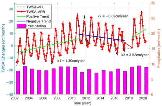
Figure 2.
Monthly changes of GRACE-derived TWSAVFL and TWSAVRB, respectively, over Volta Fractured Land and Volta River Basin, and Annual precipitation changes within the basin from 2002 to 2020. Volta Fractured Land represents the Lake Volta and Bui reservoir catchment.

Table 1.
Annual Amplitude and Phase of TWSAVRB and Precipitation.
As precipitation is the main input for water resources within the VRB, it is worth giving an overview of the influences of hydrological conditions on precipitation changes. Figure 3 is a juxtaposition of precipitation and the drought index for the study period. It shows a similarity between temporal variability in both PDSI and annual precipitation anomalies over the Volta River Basin, where negative and positive values of PDSI, respectively, describe hydrological dry and wet conditions. During the drought period from 1970 to 1991/92, which reached its peak in 1983, (as indicated by the negative values of PDSI), the annual rainfall anomalies were continually negative. The period from 1993 to 2000 was characterized by a mix of both drought and wet seasons. Because of the dominant drought episode in the period from 2001 to 2007, annual precipitation anomalies were constantly negative, while significant positive anomalies were found in 2003. Annual precipitation anomalies consistent with PDSI values, were continuously positive from 2008 to 2011, before becoming negative from 2012 to 2016.
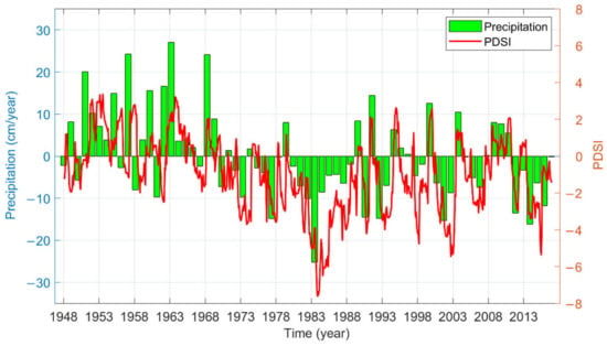
Figure 3.
Annual precipitation anomalies relative to mean precipitation of 1948−2016 and PDSI time-series.
4.2. Water Mass and Level Changes in Both Lake Volta and Bui Reservoir
Water height records of the main reservoirs within the VRB, i.e., Lake Volta and Bui Reservoir, are presented in Figure 4. Lake Volta mainly experienced a rise in lake level during 2007–2011 and 2016–2019, and a decline during 2011–2016. Indeed, a total rise of 12.56 m occurred from July 2007 to November 2011, with a mean rising rate of over 0.23 m/month. In addition, a total rise of 9.41 m was observed from June 2016 to November 2019, with a mean rising rate of over 0.22 m/month. Furthermore, a total decline of −11.75 m occurred from November 2011 to June 2016, with an average declining rate of over −0.20 m/month. Another less evident decline of −6.56 m was observed from November 2003 to July 2007, with an average decline rate of −0.14 m/month. The seasonal changes in lake water level often reached their minimum and maximum values in June and November, respectively. It is worth pointing out that changes in level for Lake Volta in 2012 showed an increase of 0.1 m between February and October, but a decrease of −0.58 m between January and December. These suggest that Lake Volta presented no significant water level changes in 2012.
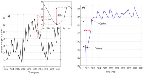
Figure 4.
Radar altimetry-derived monthly water level records above sea level (a.s.l.) for (a) Lake Volta and (b) Bui reservoir. The dotted red box displays the inset of monthly water level time-series of the Lake Volta in 2012.
Figure 4b presents the water level changes in the Bui Reservoir from October 2011 to 2021. It is worth recalling that the construction of the main Bui dam, which impounds Bui reservoir, began in December 2009, after the Black Volta River diversion was achieved in December 2008. Then, the Bui reservoir impoundment process specifically started in June 2011. In contrast to Lake Volta, Bui Reservoir presented a rapid water level increase in 2012 (Figure 4b). After impounding water continuously for eight months, there was a total increase of about 34.4 m from February to October in 2012 with a mean rising rate of about 4.3 m/month. After 2012, the water level displayed either a balanced or a declining trend and was associated with significant seasonal variations of 12 m maximum.
As Lake Volta and Bui reservoir are the main water reservoirs within the VRB (Figure 1), their changes in surface water storage were estimated by combining altimetry and imageries data to accurately segregate the changes in GWSA. It is worth recalling that level records for Lake Volta during 2002 to 2020 were derived from satellite altimetry, while the area changes were derived from Landsat 7/8 imageries for the period of 2003 to 2016. Therefore, we used the lake level changes over 2003–2016 to retrieve the geometric link (Figure 5a) between the changes in the lake level and surface area. Because geometric equation accuracy is highly related to the time delays between the day of the month in which the images and water levels were recorded, a time delay of 5 days was adopted. Therefore, the images and the corresponding water level records that are not within this time delay were then eliminated to improve the accuracy of the regression model (Figure 5a). There was a significant linear correlation (R2 = 0.934) between the lake water height and surface area changes.
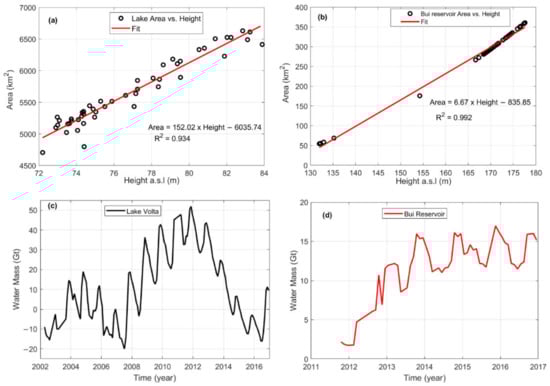
Figure 5.
Regression models between radar altimetry-derived water level and imageries-derived water area changes: (a) for Lake Volta and (b) Bui Reservoir. Estimated surface water mass changes based on water area-height relationship for (c) Lake Volta and (d) Bui reservoir from 2002 to 2016 and 2011 to 2016, respectively.
Furthermore, the Hydroweb-estimated level and area changes for Bui reservoir from October 2011 to July 2020 were applied to retrieve the geometric link between the changes in level and area in the Bui reservoir. Similarly, the reservoir’s surface areas and the corresponding water levels of the same day of the month are used to recover the area-height relationship presented in Figure 5b. There was a good linear correlation between the Bui reservoir water height and area changes, with R2 = 0.992.
Once both Lake Volta and Bui reservoir area-height relationships were derived, the monthly changes in their water area or level can be retrieved based on the radar altimetry water height observations or imageries-derived water area. The monthly changes in their respective water area and height were then combined using the Equation (2) to recover their respective monthly water mass changes. Lake Volta and Bui Reservoir’s water mass changes are presented in Figure 5c,d.
Obviously, changes in the lake water mass increased and decreased over 2002–2016. The most noticeable features in Figure 5c are the water mass rise from 2007 to 2011 and decline over 2012–2016. Indeed, a total mass rise of 71.86 Gt occurred from July 2007 to November 2011, with a mean rising rate of over 1.35 Gt/month. Conversely, a total decline of −67.95 Gt occurred from November 2011 to June 2016, with an average declining rate of over −1.21 Gt/month. Another less evident decline of −34.54 Gt was observed from November 2003 to July 2007, with an average decline rate of −0.76 Gt/month. In contrast to the Lake Volta, the Bui reservoir presented a total mass rise of 13.29 Gt from October 2011 to December 2013, with a mean rising rate of ~0.49 Gt/month (Figure 5d). In addition, the Bui reservoir water mass displayed either a balanced or a declining trend after 2013, and was associated with significant seasonal variations up to ~6 Gt.
Furthermore, surface water storage changes for Lake Volta and Bui reservoir were then obtained by dividing each month’s water mass by the standard average areas for the lake and the reservoir, which were ~8500 km2 and ~222 km2, respectively. To be consistent with GRACE data, the estimated surface water storage changes were filtered in the same way as the GRACE data. The filtered SWSA changes can then be obtained by adopting the same baseline (2004–2009) as the GRACE data.
4.3. Influences of Bui Reservoir Operation on Changes in TWSAVRB in Spatial Domain
To investigate the influences of the Bui Reservoir operation on changes in the spatial domain for TWSAVRB, the original GRACE Stokes coefficients were converted to mass changes after replacing the first-degree and C20 coefficients by more consistent estimations [55,56]. The estimated mass changes in this section were free from any decorrelation filter and smoothing that would degrade the signals of Bui Reservoir impoundment in the spatial domain. However, before using these unfiltered and unsmoothed mass changes, it is worth comparing them to those that are filtered and/or smoothed.
Figure 6 shows the spatial pattern of GRACE-observed mass variations within the VRB between February and November in 2012, when the Bui Reservoir water level rapidly increased (Figure 4b), using GRACE original Stokes coefficients and different filters (G300, DDK8 and P4M6 + G150). Obviously, all four results display an overall positive trend in the GRACE-observed mass variations over the surrounding area of Bui Reservoir. Higher amplitude of mass variations was observed in GRACE original data (Figure 6a) and DDK8 (Figure 6c), while lower amplitude of mass variations was seen in G300 (Figure 6b) and P4M6 + G150 (Figure 6d). A filter method is generally applied to suppress noise and correlated errors in GRACE original data. Therefore, the observed signals in such G300 (Figure 6b) and P4M6 + G150 (Figure 6d) could be attributed to the rapid increase in the Bui Reservoir water level. The G300 and P4M6 + G150 filters are stronger than the DDK8 filter, suggesting that signals in DDK8 could be affected by noise and correlated errors, as similar amplitude was seen in the GRACE original data (Figure 6a) and DDK8 (Figure 6c). The main conclusion from Figure 6 was that the quick water level increase in Bui reservoir in 2012 might have been captured by the GRACE satellites.
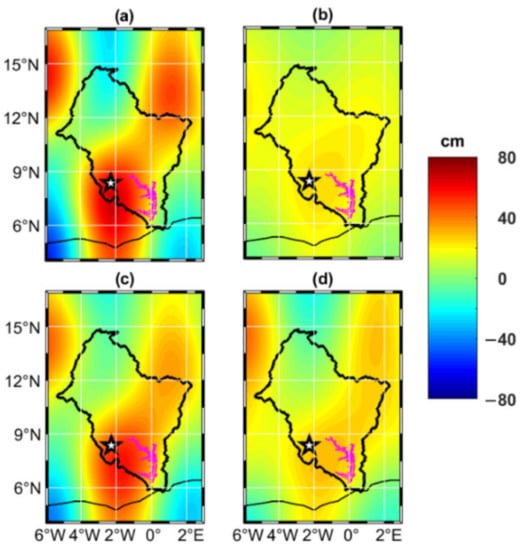
Figure 6.
GRACE-observed mass changes between February and November in 2012 (Bui Reservoir impoundment). The raw (a) GRACE estimate is compared with (b) a 300 km Gaussian filtered GRACE estimate, (c) a DDK8 filtered GRACE estimate, (d) a combination of the decorrelation filter P4M6 and a 150 km Gaussian filter. The location of the Bui Reservoir is marked with a white star. The pink area represents the Volta Lake.
Even though signals in Figure 6a were highly contaminated by noise and correlated errors, the corresponding mass changes were kept in the following analysis of this section. The mass changes from the GRACE original data were adopted to avoid the signals deterioration that could be induced by a filter method over the surrounding area of Bui Reservoir.
The monthly changes in Raw TWSAVRB (RTWSAVRB) derived from the GRACE original data with seasonal variations removed in 2012 are presented in Figure 7. ‘Raw’ means that the original GRACE Stokes coefficients were converted into mass anomalies changes after replacing the first-degree and C20 coefficients by more consistent estimations. The average mass over the first 4 months in 2012 was taken as the reference and was deducted from all the other monthly grids. According to the water level changes in Figure 4b, RTWSAVRB was expected to rapidly increase from February 2012 to November 2012 over the surrounding area of Bui Reservoir, reaching a maximum in November 2012. Obviously, the observations in March-August 2012 were largely contaminated by north-south oriented striped noise. However, positive RTWSAVRB changes were generally discernible after September 2012, except in December 2012. As seen in Figure 4b, the water level also displayed significant seasonal variations up to 12 m after 2012. The seasonal variations generally reached their trough and peak values in June and November, respectively.
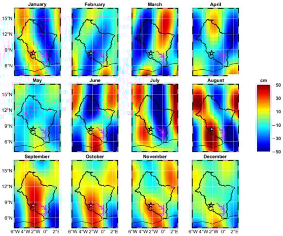
Figure 7.
The raw GRACE estimated monthly mass changes with seasonal variations removed during the period from January 2012 to December 2012. All the plots have been deduced from the mean of the first 4 months in 2012. The location of the Bui Reservoir is marked with a white star. The pink area represents the Volta Lake.
The estimated monthly changes in RTWSAVRB were further averaged over September-November (Figure 8) to deeply investigate how GRACE observes the mass changes over the surrounding area of Bui Reservoir before and after the Bui dam construction. As seen from Figure 8, no significant signals were generally apparent around the Bui Reservoir area before 2007. A significant positive RTWSAVRB grew from 2008 to 2012, before decreasing after 2012. Indeed, as the impoundment of the Bui reservoir began in December 2009 after the Black Volta River diversion was achieved in December 2008, this could be responsible for the observed positive RTWSAVRB in 2008 over the surrounding areas. Furthermore, the reservoir impoundment process specifically started in June 2011, and the dam was commissioned for use in December 2013. The observed strong positive RTWSAVRB in 2012 could certainly be induced by the rapid increase in the water level of Bui Reservoir. These consecutive observations from the GRACE original data approximately indicate that the evolutions of RTWSAVRB over the surrounding area of Bui Reservoir were mainly as a consequence of water impoundment caused by the Bui reservoir operation.
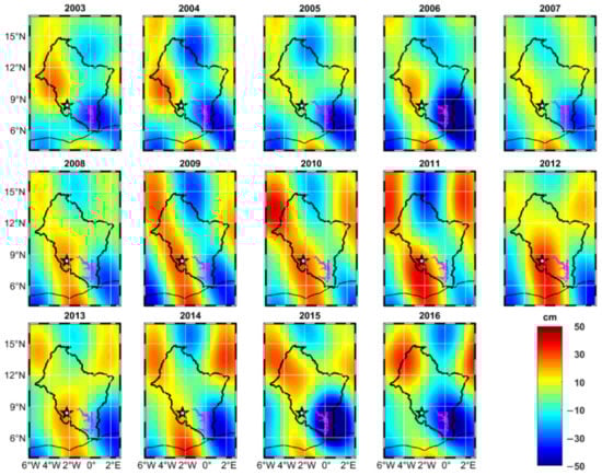
Figure 8.
Multi-year averages of raw GRACE estimated mass changes in SeptemberNovember from 2003 to 2016 with seasonal variations removed. All the plots have been deduced from the mean of the first 4 months in 2012. The location of the Bui Reservoir is marked with a white star. The pink area represents the Volta Lake.
4.4. Influences of Bui Reservoir Operation on Changes in TWSAVRB Detected by GRACE in Spectral Domain
Figure 9 displays the monthly and multi-year averages of precipitation, GRACE-observed and WGHM-derived TWSAVRB. It is worth highlighting that the WGHM predictions did not include the Bui Reservoir impoundment, as the global database of lakes and wetlands used by the WGHM does not contain the Bui Reservoir [40]. Therefore, comparing the GRACE-observed TWSAVRB with the WGHM-derived TWSAVRB could help in understanding whether the Bui Reservoir impoundment can be captured by GRACE satellites. As seen in Figure 9a,b, the precipitation in July-September accounted for more than 56% of the total annual precipitation, suggesting that precipitation in the VRB was mainly concentrated in July-September. From 2003 to 2010, monthly precipitation reached its maximum in August, with an average value of 21.33 cm (Figure 9a). Similarly, the maximum of monthly precipitation during 2011–2016 was up to 18.77 cm in August (Figure 9b), showing that the precipitation decreased during this period.
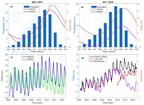
Figure 9.
Monthly mean time-series of GRACE-observed TWSAVRB, WGHM-derived TWSAVRB and precipitation derived from Global Precipitation Climatology Centre in the VRB area computed for two periods: (a) 2003–2010 and (b) 2011––2016; (c) monthly time-series of GRACE-observed and WGHM-derived TWSAVRB over 2002–2016; (d) difference between GRACE-observed TWSAVRB and WGHM-derived TWSAVRB, monthly time-series of altimetry-imageries-derived SWSA for both Lake Volta and Bui Reservoir.
Obviously, the monthly changes in GRACE and the WGHM-derived TWSAVRB had similar patterns before 2010, while the GRACE-observed TWSAVRB presented higher amplitude than the WGHM-derived TWSAVRB after 2010 (Figure 9c). Indeed, during the 2003–2010 period, when the Bui reservoir impoundment had not started, the monthly mean changes of GRACE and the WGHM-derived TWSAVRB reached their maximum in September with average values of 13.94 cm and 11.73 cm, respectively (Figure 9a). In addition, monthly WGHM-derived and GRACE-estimated TWSAVRB reached their minimum in March and April, with average values of −5.15 cm and −9.58, respectively. The annual amplitudes of GRACE-observed and WGHM-derived TWSAVRB, respectively, were ~11 cm and ~8 cm, while their annual phases for the same period were ~9 and ~7, respectively. The differences between these annual amplitudes and phases can be related to the fact that certain physical processes may be ignored in WGHM predictions [64].
Furthermore, during the 2011–2016 period, when the Bui Reservoir impoundment began, the monthly mean changes of GRACE and the WGHM-derived TWSAVRB reached again their maximum in September with average values of 16.89 cm and 5.15 cm, respectively (Figure 9b). During this period, the annual amplitudes of GRACE and the WGHM-estimated TWSAVRB were, respectively, ~9 cm and ~7 cm; whereas they reached their minimum in April with average values of −1.73 cm and −9.18 cm, respectively. Clearly, the decreased precipitation in 2011–2016 was reflected in both GRACE and the WGHM-derived TWSAVRB signals, as the latter presented lower annual amplitudes in 2011–2016 (~9 cm and ~7 cm) than in 2003–2010 (~11 cm and ~8 cm). In addition, the WGHM-estimated TWSAVRB presented lower monthly average values in 2011–2016 with respect to the precipitation patterns. The WGHM-derived TWSAVRB ranged between −9.18 and +5.15 in 2011–2016, whereas they changed between −5.15 cm and +11.73 cm in 2003–2010. The GRACE-observed TWSAVRB, in contrast, displayed higher monthly average values in 2011–2016. The changes in the GRACE-observed TWSAVRB ranged between −1.73 cm to 16.89 cm in 2011–2016, while they ranged between −9.58 cm to 13.94 cm in 2003–2010. Clearly, the multi-year averages of the monthly GRACE time series in 2011–2016, when the Bui Reservoir impoundment began, displayed an overall increasing trend; indicating storage increase in regional hydrology. In contrast, the WGHM time series did not display any trend, indicating no storage increase in regional hydrology.
To deeply understand the observed disparities between the GRACE and the WGHM-derived TWSAVRB during 2011–2016, the difference between their monthly time series was then compared to the surface water storage anomalies for Lake Volta and Bui reservoir (Figure 9d). It is worth recalling that the estimated surface water storage changes were filtered in the same way as the GRACE data. In addition, the filtered SWSA changes presented in Figure 9d were then obtained by adopting the same baseline (2004–2009) as GRACE data for the Lake Volta, while the first four months in 2012 were used as the baseline for the Bui reservoir. Obviously, the increasing trend in the residuals (GRACE-WGHM) during 2011–2016 was mainly related to the Bui reservoir impoundment (Figure 9d). Finally, it was concluded that TWSAVRB changes were affected by the Bui Reservoir operation.
4.5. Temporal Variations of Water Storages within the Volta Fractured Land
Figure 10 presents the monthly, seasonal, and de-seasonal changes in TWSAVFL, as well as in water components, including Altimetry-imageries estimated SWSA, GLDAS-derived SMSA and GRACE-derived GWSAVFL within the Volta Fractured Land from 2002 to 2016. The de-seasonalized temporal components that dominated the interannual variability were obtained by removing the linear trend and seasonal signals from the raw series. To avoid the probable surface water underestimation from other lakes/reservoirs within the basin, the GRACE-derived GWSAVFL time series analysis in this study was focused on the Volta Fractured Land, which contains the main Lake Volta and Bui reservoir (Figure 1). As the WGHM model does not include water storage in the Bui reservoir, the GRACE-derived GWSAVFL were obtained by combining SMSA from GLDAS outputs and altimetry-imageries-derived SWSA over the Volta Fractured Land. The altimetry-imageries-derived SWSA presented in Figure 10b were obtained by combining estimated changes in surface water storage for both Lake Volta and Bui reservoir. It is worth recalling that the altimetry-imageries estimated SWSA and GLDAS-derived SMSA were filtered in the same way as the GRACE data.
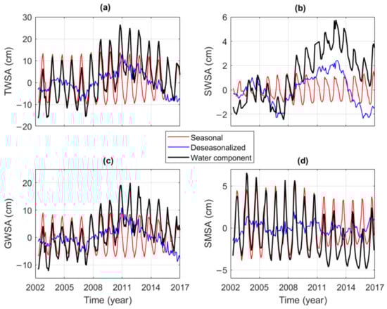
Figure 10.
Temporal component time series of (a) TWSAVFL; and water component from (b) Altimetry−imageries estimated SWSA, (c) GWSAVFL and (d) GLDASderived SMSA. The altimetryimageriesderived SWSA were obtained by combining both Lake Volta and Bui reservoir estimated surface water storage changes. Monthly time series of water storages were de-seasonalized by removing the linear trend and seasonal signals. The seasonal component in each water storage was derived by applying the seasonal and trend decomposition using the loess (STL) algorithm while the linear trend was estimated using the least square fitting approach. All the time series were averaged over Volta Fractured Land from 2002 to 2016.
It can be seen from Figure 10a that the seasonal component of the TWSAVFL presented significant constant amplitude from 2002–2010, before slightly decreasing after 2010. However, its interannual variability decreased and increased, respectively, during 2003–2007 and 2007–2010, before decreasing again from 2011–2016. The seasonal variability and long-term (interannual variability + linear trend) contributions were estimated to be ~52% and ~40%, respectively. It was concluded that the changes in the TWSAVFL depend on both seasonal and interannual variability. It is worth recalling that the TWSAVFL signals were similar to the TWSAVRB, representing about ~83% of those at basin scale, suggesting that the TWSAVRB is largely dependent on the TWSAVFL (see Section 4.1 for details).
Figure 10b shows that monthly changes in SWSA decreased and increased during 2003–2006 and 2007–2012 at rates of −0.21 ± 0.16 cm/year and 1 ± 0.07 cm/year, respectively, before decreasing again from 2013 to 2016 with a rate of −0.84 ± 0.16 cm/year. Similarly, the interannual component of SWSA decreased and increased, respectively, during 2003–2006 and 2007–2012, before decreasing again after 2012. However, its seasonal component generally presented a constant amplitude over the study period. The SWSA’s seasonal and long-term variability (interannual variability + linear trend) contributions were estimated to be ~67% and ~26%, respectively. It can be concluded that SWSA changes mainly depend on the interannual variability.
Figure 10c shows that the GWSAVFL was almost stable from 2002 to 2006, before increasing and decreasing during 2006–2011 and 2012–2016, with rates of 2.67 ± 0.34 cm/year and −1.80 ± 0.32 cm/year, respectively. A recent study by Resende et al. [35] revealed that the groundwater storage increased from 2006 to 2011 based on groundwater level records from shallow wells that were located in the proximity of Lake Volta (generally <20 km) within the Volta Fractured Land. This is consistent with the observed results in this study. In addition, Figure 10c shows that the interannual component of GWSAVFL increased and decreased, respectively, during 2007–2010 and 2011–2016. However, its seasonal component generally presents constant amplitude over the study period. The seasonal variability and long-term (interannual variability + linear trend) contributions were estimated to be ~46% and ~44%, respectively. It can be concluded that the changes in the GWSAVFL depend on both seasonal and interannual variability.
Figure 10d shows that SMSA decreased over the study period at a rate of −0.27 ± 0.03 cm/year. It seems that the SMSA presented no significant interannual changes during 2002–2016. However, significant seasonality was observed during the study period. In term of percentage, the long-term variability and seasonality contributions of SMSA were estimated to be ~30% and ~61%, respectively. It was concluded that the changes in SMSA mainly depend on the seasonal variability.
To thoroughly understand the water components influences, their contributions were also quantified. This revealed that the contributions of SWSA, GWSAVFL and SMSA were ~19%, ~57%, and ~24%, respectively, within Volta Fractured Land. In addition, the contributions of SWSA, GWSAVFL, and SMSA were ~12%, ~62%, and ~26%, respectively, within the VRB. A study by Ferreira and Asiah [65] reported that the contribution of the changes in surface water storage in Lake Volta was about 48% of the terrestrial water storage changes within the VRB. Similarly, Ndehedehe et al. [25] estimated that contribution to be about 41% of the basin’s terrestrial water storage changes. However, Ferreira et al. [21] highlighted the contribution from Lake Volta to be around 8.8% within the VRB, which is in agreement with the finding value in this study. It is worth highlighting that previous studies did not include the new Bui reservoir storage nor storage changes from soil moisture and groundwater. Ferreira et al. [21] have attributed the difference between their result and those from the previous studies to the methodology applied. According to the previous findings (41%, 48%, and 8.8%), a mean value of the Lake Volta contribution can be estimated for about ~32.6%. Therefore, the estimated contribution of both Lake Volta and Bui reservoir in this study represents about ~37% of previous findings within the VRB. In addition, it can be concluded that GWSA is the main water component in the VRB as well as in Volta Fractured Land.
5. Discussion
5.1. Water Storage Changes Influenced by Natural Causes
Decrease in precipitation and/or increase in temperatures over time results in a decline of terrestrial water storage due to decreased accumulation of water in various lakes/reservoirs and increased evaporation, and vice versa [3]. As found in Section 4.1, the changes in precipitation which govern the changes in TWSAVRB were largely influenced by the hydro-meteorological conditions (e.g., floods and droughts). This suggests that the temporal changes in freshwater could be likely impacted by severe hydro-meteorological conditions (e.g., floods and droughts), as rainfall is the main input of the TWSAVRB. Therefore, studying the relationships between the variability of TWSAVRB and climatic indices helps to reveal the periods of impacts of large-scale climate indices. This is helpful for understanding the trends in GWSAVFL as well as changes in TWSAVRB under climate influences. In this case, the cross-wavelet transform method was applied to characterize the influences of ENSO, AMO, and AMM events on the changes in TWSAVRB during 2003–2016. The cross-wavelet analyses between the monthly TWSAVRB and the monthly climate teleconnections are presented in Figure 11. The relative phase correlation (with negative phase pointing left and positive phase pointing right) is expressed by the arrows, and the contours indicate the 5% significance level against red noise. The energy density is showed by the color bar.
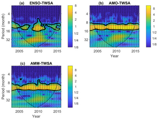
Figure 11.
Cross wavelet transforms between TWSAVRB and (a) ENSO, (b) AMO and (c) AMM from 2003 to 2016 in the Volta River Basin. The relative phase relationship is denoted as arrows (with anti-phase pointing left, in-phase pointing right). The color bar on the right denotes the wavelet energy.
It can be clearly seen in Figure 11a that ENSO had a statistically significant negative correlation with the TWSAVRB at the 5% significance level, with a 9–15 month period signal in 2008–2012. In addition, ENSO and the TWSAVRB had a positive phase correlation in 2004–2008 and 2012–2015, with 9–13 and 11–13 month period signals, respectively. These statistically significant positive and negative correlations directly indicate that ENSO events exert an influence on changes in the TWSAVRB. It is obvious from Figure 11b that AMO events had a significant positive correlation with the TWSAVRB, with a 9–13 month period signal in 2004–2008 and 2012–2015. Similarly, Figure 11c indicates a significant positive correlation between the AMM events and the TWSAVRB, with a 9–13 month signal period from 2004 to 2015. These statistically significant positive correlations directly indicate that AMO and AMM events exert an important influence on changes in the TWSAVRB.
Indeed, the results of the cross wavelet transforms application indicated that global climate teleconnection indices exert an influence on the TWSAVRB changes. This analysis revealed three main sub-periods of climate impacts, which are: 2004–2008, 2008–2012 and 2012–2016. It was observed that significant correlations of ENSO and AMO with the TWSAVRB generally fell within these periods. The observed correlation zones of ENSO agree with strong La Niña (https://ggweather.com/enso/oni.htm, accessed on 10 January 2022) episodes (e.g., 2007–2008 and 2010–2011) and a strong El Niño (https://ggweather.com/enso/oni.htm, accessed on 10 January 2022) episode in 2014–2015. Strong El Niño episodes commonly lead to extreme dry events, whereas strong La Niña episodes usually lead to severe wet conditions in this region. The positive (negative) correlation between ENSO and the TWSAVRB (see Figure 11a) corresponds with decreasing (increasing) TWSAVRB (Figure 2) and GWSAVFL (Figure 10c). For instance, positive and negative correlations were found between ENSO and the TWSAVRB in 2004–2008 and 2008–2012, respectively; when the TWSAVRB decreased and increased from 2004 to 2006 and 2006 to 2011, respectively (Figure 2). The linear trends in the TWSAVRB and GWSAVFL changes under severe climate influences were also estimated. Results revealed that the TWSAVRB and the GWSAVFL increased from 2006 to 2010 at a rate of 2.90 cm/year and 3.75 cm/year, respectively. In addition, changes in the TWSAVRB and GWSAVFL, respectively, presented negative trends of −1.25 cm/year and −1.75 cm/year from 2011 to 2016. It can be assumed that the strong episodes of La Niña in 2007–2010, and El Niño in 2014–2015 have impacted the changes in the TWSAVRB and GWSAVFL.
Furthermore, a time lag range of 0–120 months was applied to investigate the link among the interannual time series of ENSO, TWSAVRB and GWSAVFL from 2007 to 2016, to better understand how changes in the TWSAVRB and GWSAVFL were affected by severe ENSO episodes (Figure 12). The interannual time series were obtained by removing the linear trend from the long-term time series. Figure 12 indicates that the maximum correlation coefficient between the TWSAVRB and strong ENSO events was −0.71, with a lag of 3 months. The maximum correlation coefficient between the GWSAVFL and strong ENSO episodes was −0.78, with a lag of about 6 months. The interannual time series in the TWSAVRB and GWSAVFL have a maximum correlation coefficient of 0.97, with a lag of 0 month. It has been reported that precipitation patterns and hydro-meteorological conditions are largely influenced by the large-scale ocean-land-atmospheric interchanges and global climate teleconnections (e.g., ENSO), which then control the TWSA changes within the VRB [12,13,17,24,25,26]. As found in Section 4.1, precipitation and the TWSAVRB had almost the same annual amplitudes of about 9–10 cm, which peaked around June and September, respectively. That suggests a delay of 3 months between their annual amplitude’s peaks. The same time lag can be observed among the interannual changes of strong ENSO events and TWSAVRB. The strong correlation coefficients among the strong ENSO, and interannual variabilities of TWSAVRB and GWSAVFL suggests that the severe ENSO events affected the TWSAVRB and GWSAVFL interannual changes through precipitation. Ndehedehe et al. [18] investigated terrestrial water storage changes in Western Africa’s basins under the global climate teleconnections influences, and found out that GRACE-based terrestrial water storage changes seem to be more related to ENSO events over the VRB. For instance, the La Niña strong events in 2007–2008 and 2010–2011, were retrieved among the temporal evolutions of their estimated Standardized Precipitation Index with 6-month timescales, during which severe wet conditions were observed in 2010, accompanied by a significant amplitude of terrestrial water storage within the VRB. This suggests that the ENSO events affected the precipitation patterns with a lag of 6 months over the VRB. A recent study by Li and Rodell [66] showed that the groundwater drought index presented a better correlation with the 6-month timescales Standardized Precipitation Index within a shallow aquifer, suggesting that the groundwater storage changes respond to the shorter term of precipitation changes. According to these observations, it can be concluded that the effect of strong ENSO events on the GWSAVFL interannual variability within the basin is short-term, with a lag of 6 months.
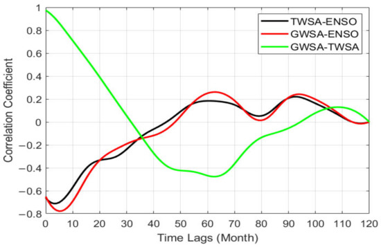
Figure 12.
Correlations among the interannual changes of ENSO, TWSAVRB and GWSAVFL from 2007 to 2016. The interannual time series were obtained by removing the linear trend from the long-term time series. The linear trends were estimated using the least square fitting approach while the long-term time series were derived by applying the seasonal and trend decomposition using loess (STL) algorithm.
5.2. Surface Vegetation Dynamics from NDVI as Proxy for Infrastructure Influences on Water Storage Changes
Ndehedehe et al. [51] investigated hydrological influences on vegetation dynamics within West Africa catchments using Global Inventory Modelling and Mapping Studies (GIMMS) based on NDVI and GRACE-derived terrestrial water storage from 2002 to 2013. Their results revealed a stronger association between temporal GIMMS-derived NDVI and GRACE-derived terrestrial water storage than that widely reported between NDVI and precipitation, suggesting that West Africa vegetation dynamics were controlled by terrestrial water storage. As found in Section 4.5, the GWSAVFL are the main water component in the GRACE-derived TWSAVRB within the VRB. Therefore, it can be suspected that surface vegetation dynamics in this area are also controlled by the GWSAVFL. A recent study by Bhanja et al. [50] revealed that NDVI might be employed as a suitable groundwater storage changes indicator in areas with shallow aquifer and natural vegetation such as the VRB (or Volta Fractured Land).
Indeed, the Lake Volta and Bui reservoir impoundments during periods of heavy and constant rain will increase shallow aquifers recharge within Volta Fractured Land. In other words, the water impoundments behind the Akosombo and Bui dams during the strong and constant rain season will increase the long-term groundwater storage, which could have long-term effects on the surface vegetation. Therefore, seasonal, and long-term (linear + interannual) variations of the TWSAVFL, GWSAVFL, precipitation and NDVI estimated using the STL method (see Section 3.4) are presented in Figure 13 and Figure 14, respectively. It is worth recalling that the NDVI and precipitation anomalies were estimated using the same baseline (2004–2009) as the GRACE data.
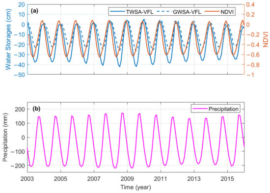
Figure 13.
Cumulative monthly seasonal variations of (a) water storage from TWSAVFL (blue curve) and GWSAVFL (dashed blue curve), and NDVI (red curve); (b) precipitation from 2003 to 2016. The seasonal components were estimated using the STL method.
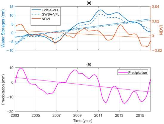
Figure 14.
Monthly long-term variations of (a) water storage from TWSAVFL (blue curve) and GWSAVFL (dashed blue curve), and NDVI (red curve); (b) precipitation from 2003 to 2016. The long-term (linear + interannual) components were obtained using the STL method. Derived linear Trends using least square fitting approach are presented as line or dashed line.
As seen in Figure 13a, cumulative seasonal changes in GWSAVFL were generally similar to those of TWSAVFL with a strong correlation coefficient of 0.99. In addition, it seems that the NDVI seasonal changes were associated with the seasonal variations of both TWSAVFL and GWSAVFL (Figure 13a) with relative correlation coefficients of 0.58 and 0.52, respectively. However, a strong correlation coefficient of 0.90 was found between cumulative seasonal changes of NDVI and precipitation, indicating that seasonal changes in NDVI were highly associated with the seasonal variations of precipitation (Figure 13a,b). It can be concluded that precipitation, TWSAVFL, and GWSAVFL control the seasonal changes in NDVI, while precipitation is the highest factor influencing the seasonal variations in NDVI.
Obviously, long-term variations in the GWSAVFL were generally like those of TWSAVFL (Figure 14a), with a strong correlation coefficient of 0.98. Figure 14a shows that changes in both the TWSAVFL and GWSAVFL increased in recent years, while the precipitation and NDVI decreased (Figure 14a,b). Indeed, the monthly long-term variations of both the TWSAVFL and GWSAVFL increased and reached their maximum, respectively, in 2011, before decreasing after 2011. Apart from its maximum value in 2003, the monthly long-term changes in NDVI reached its second highest and minimum values in 2013 and 2015, respectively. In addition, Figure 14a indicates that long-term changes in NDVI significantly increased over 2012, while the precipitation decreased in recent years. Furthermore, a slight increase was also observed in the monthly long-term variations of both the TWSAVFL and GWSAVFL over 2012. It is worth recalling that contrary to the TWSAVFL and GWSAVFL, the NDVI time series were not filtered. This suggests that filtering significantly suppressed signals in the GRACE-derived TWSAVFL and GWSAVFL. As found in Section 4.3, water storage decreased around Lake Volta, while it significantly increased around Bui reservoir in 2012. The observed signals over the surrounding area of Bui Reservoir were mainly because of water impoundment caused by the Bui reservoir operation. Obviously, the Bui reservoir water impoundment was reflected in the NDVI changes. One can assume that the increase of NDVI signals in 2012 could be related to the Bui Reservoir operation.
We note that the surface water storage could not directly affect the surface vegetation unless through recharge. Indeed, recharge of local and shallow aquifers such as in Volta Fractured Land is largely controlled by infiltration from the new reservoir water impoundment, the precipitation and surface-water/river interchange [35]. Therefore, analyzing the relationship between the long-term changes in NDVI, TWSAVFL and GWSAVFL could help to better understand how water storages affect the surface vegetations changes in this area. Obviously, there is no significant association between long-term changes in precipitation and NDVI, as the cumulative long-term variations of both NDVI and precipitation have a poor correlation coefficient of 0.33. However, cumulative long-term variations of both TWSAVFL and NDVI present a relatively strong correlation coefficient of 0.70, suggesting that NDVI long-term changes were associated with the long-term variations of the TWSAVFL. In addition, cumulative long-term variations of both the GWSAVFL and NDVI present a relative correlation coefficient of 0.67, indicating that the NDVI long-term changes were also associated with the long-term variations of GWSAVFL.
6. Conclusions
The operation of Bui reservoir and the recent climate changes have significantly influenced the water storage changes within Volta River Basin. The influence of the largest manmade lake (Lake Volta, with about 8500 km2 area) in Volta River Basin, in West Africa has largely been reported by previous studies. For instance, it is reported that Lake Volta contributed ~41% to the observed Volta River Basin’s TWSA in 2002–2014. Recent studies revealed that water storage changes in the ~400 km2 reservoir can be detected by GRACE satellites. The implementation of Bui reservoir with about 400 km2 area has occurred during the GRACE mission and therefore could be monitored from space. For the first time, this study applied GRACE and global hydrology model data to investigate the influence of the Bui reservoir operation on water storage variations within Volta River Basin. The WaterGAP model (WGHM) was selected because it does not include water storage in the Bui reservoir. In addition, variation in groundwater storage was also estimated by combining GRACE-derived TWSA, radar altimetry records and Landsat images derived Lake Volta and Bui reservoir SWSA, and GLDAS simulated SMSA data from 2002 to 2016. Results showed that TWSA increased (1.30 ± 0.23 cm/year) and decreased (−0.82 ± 0.27 cm/year), respectively, during 2002–2011 and 2011–2016 within Volta River Basin, matching previous TWSA investigations in this area. It revealed that the multi-year averages of monthly GRACE-derived TWSA changes in 2011–2016 displayed an overall increasing trend, indicating storage increase in regional hydrology, while the Lake Volta water storage changes decreased. The GRACE minus WGHM residuals display an increasing trend in Volta River Basin water storage during the Bui reservoir operation in 2011–2016. The observed trend compares well with the estimated Bui reservoir SWSA, indicating that GRACE solutions can retrieve the true amplitude of large mass changes happening in a concentrated area, e.g., the water impoundment in the Bui reservoir area, with the help of hydrologic modeling, even though such an area is much smaller than the resolution of GRACE global solutions. In the spatial domain, the GRACE observations show significant positive mass changes over the surrounding area of Bui Reservoir because of Bui reservoir water impoundment. It also revealed that the GWSA was almost stable from 2002 to 2006, before increasing and decreasing during 2006–2011 and 2012–2016 with rates of 2.67 ± 0.34 cm/year and −1.80 ± 0.32 cm/year, respectively. The observed trends in the GRACE-derived TWSA and GWSA changes were generally attributed to the hydro-meteorological conditions (e.g., floods and droughts). This study revealed that the effects of strong ENSO events on the GWSA interannual variability within the Volta River Basin are short-term, with a lag of 6 months.
Furthermore, the contributions of water components within the Volta River Basin were estimated to be ~12% (being ~37% of previous results), ~62%, and ~26%, for SWSA, GWSA and SMSA, respectively. This suggests that the GWSA is the main water component within Volta River Basin. Temporal dynamics analysis revealed that changes in the TWSA and GWSA depend on both seasonal and interannual variabilities. The water storage changes influences on the surface vegetation dynamics within Lake Volta and Bui reservoir catchments were also investigated in this study using MODIS-derived NDVI. Results revealed that the seasonal changes in NDVI were associated with the seasonal variations of both TWSA and GWSA with relative correlation coefficients of 0.58 and 0.52, respectively. A strong correlation coefficient of 0.90 was found between NDVI and precipitation cumulative seasonal changes, indicating that seasonal changes in NDVI were highly associated with the seasonal variations of precipitation. It also revealed that there was no significant association between precipitation and long-term changes in the NDVI, as the cumulative long-term variations of both NDVI and precipitation had a poor correlation coefficient of 0.33. However, cumulative long-term variations of both TWSA and NDVI had a relatively good correlation coefficient of 0.70, suggesting that long-term changes in NDVI were associated with the long-term variations of TWSA. In addition, the cumulative long-term variations of both GWSA and NDVI present a relative correlation coefficient of 0.67, indicating that the NDVI long-term changes were also associated with the long-term variations of GWSA.
Though this study used different remote sensing datasets to present the influences of Bui Reservoir operation on terrestrial water storage variation in the Volta River Basin, it was slightly limited by scarcity of consistent in situ observations. This included groundwater level and reservoir water level records. More robust techniques such as machine learning algorithms could provide more insights into the present findings, and hence, will be the focus of our future studies.
Author Contributions
Conceptualization: R.D.D., X.W. and R.F.A.; methodology: all authors; data curation: R.D.D.; funding acquisition: X.W. and S.W.; formal analysis, R.D.D.; investigation, all authors; writing—original draft preparation, R.D.D.; writing—review and editing, all authors. All authors have read and agreed to the published version of the manuscript.
Funding
This research was funded by the National Natural Science Foundation of China (No. 42074017), Open Research Fund of Qian Xuesen Laboratory of Space Technology, CAST (No.GZZKFJJ2020006), and the Fundamental Research Funds for the Central Universities (No.2-9-2022-701).
Data Availability Statement
GRACE RL06 data from Center for Space Research are available at http://icgem.gfz-potsdam.de/series (accessed on 10 January 2021). WGHM terrestrial water storage simulations can be downloaded from https://doi.pangaea.de/10.1594/PANGAEA.918447 (accessed on 10 January 2021). GLDAS outputs can be obtained from https://disc.gsfc.nasa.gov/datasets?keywords=GLDAS (accessed on 10 January 2021). AMM, ENSO and AMO time series can be downloaded from https://psl.noaa.gov/data/climateindices/list/ (accessed on 10 January 2021). PDSI data can be downloaded from https://psl.noaa.gov/data/gridded/data.pdsi.html (accessed on 10 January 2021). The Lake Volta and Bui reservoir height records can be obtained from https://hydroweb.theia-land.fr (accessed on 1 May 2022). Global MOD13A3 NDVI data and Landsat images are available at https://earthexplorer.usgs.gov/ (accessed on 5 April 2022).
Acknowledgments
We thank Hannes Mueller-Schmied for the WGHM data simulations and CSR for providing the GRACE time variable gravity field models.
Conflicts of Interest
The authors declare that the research was conducted in the absence of any commercial or financial relationships that could be construed as a potential conflict of interest.
References
- Roudier, P.; Ducharne, A.; Feyen, L. Climate Change Impacts on Runoff in West Africa: A Review. Hydrol. Earth Syst. Sci. 2014, 18, 2789–2801. [Google Scholar] [CrossRef]
- Roudier, P.; Sultan, B.; Quirion, P.; Berg, A. The Impact of Future Climate Change on West African Crop Yields: What Does the Recent Literature Say? Glob. Environ. Chang. 2011, 21, 1073–1083. [Google Scholar] [CrossRef]
- Ahmed, M.; Sultan, M.; Wahr, J.; Yan, E. The Use of GRACE Data to Monitor Natural and Anthropogenic Induced Variations in Water Availability across Africa. Earth-Sci. Rev. 2014, 136, 289–300. [Google Scholar] [CrossRef]
- Andam-Akorful, S.A.; Ferreira, V.G.; Ndehedehe, C.E.; Quaye-Ballard, J.A. An Investigation into the Freshwater Variability in West Africa during 1979–2010: Investigation of Freshwater Variability in West Africa. Int. J. Climatol. 2017, 37, 333–349. [Google Scholar] [CrossRef]
- Keenan, R.J.; Reams, G.A.; Achard, F.; de Freitas, J.V.; Grainger, A.; Lindquist, E. Dynamics of Global Forest Area: Results from the FAO Global Forest Resources Assessment 2015. For. Ecol. Manag. 2015, 352, 9–20. [Google Scholar] [CrossRef]
- Mul, M.; Obuobie, E.; Appoh, R.; Kankam-Yeboah, K.; Bekoe-Obeng, E.; Amisigo, B.; Logah, F.Y.; Ghansah, B.; McCartney, M. Water Resources Assessment of the Volta River Basin; International Water Management Institute (IWMI): Colombo, Sri Lanka, 2015. [Google Scholar]
- Yidana, S.M.; Vakpo, E.K.; Sakyi, P.A.; Chegbeleh, L.P.; Akabzaa, T.M. Groundwater–Lakewater Interactions: An Evaluation of the Impacts of Climate Change and Increased Abstractions on Groundwater Contribution to the Volta Lake, Ghana. Environ. Earth Sci. 2019, 78, 74. [Google Scholar] [CrossRef]
- Döll, P.; Hoffmann-Dobrev, H.; Portmann, F.T.; Siebert, S.; Eicker, A.; Rodell, M.; Strassberg, G.; Scanlon, B.R. Impact of Water Withdrawals from Groundwater and Surface Water on Continental Water Storage Variations. J. Geodyn. 2012, 59–60, 143–156. [Google Scholar] [CrossRef]
- Pfister, S.; Bayer, P.; Koehler, A.; Hellweg, S. Projected Water Consumption in Future Global Agriculture: Scenarios and Related Impacts. Sci. Total Environ. 2011, 409, 4206–4216. [Google Scholar] [CrossRef]
- Vörösmarty, C.J.; Douglas, E.M.; Green, P.A.; Revenga, C. Geospatial Indicators of Emerging Water Stress: An Application to Africa. Ambio 2005, 34, 230–236. [Google Scholar] [CrossRef]
- Ali, A.; Lebel, T. The Sahelian Standardized Rainfall Index Revisited. Int. J. Climatol. 2009, 29, 1705–1714. [Google Scholar] [CrossRef]
- Bader, J.; Latif, M. The 1983 Drought in the West Sahel: A Case Study. Clim. Dyn. 2011, 36, 463–472. [Google Scholar] [CrossRef]
- Diatta, S.; Fink, A.H. Statistical Relationship between Remote Climate Indices and West African Monsoon Variability. Int. J. Climatol. 2014, 34, 3348–3367. [Google Scholar] [CrossRef]
- Giannini, A.; Biasutti, M.; Held, I.M.; Sobel, A.H. A Global Perspective on African Climate. Clim. Chang. 2008, 90, 359–383. [Google Scholar] [CrossRef]
- Joly, M.; Voldoire, A. Role of the Gulf of Guinea in the Inter-Annual Variability of the West African Monsoon: What Do We Learn from CMIP3 Coupled Simulations? Int. J. Climatol. 2010, 30, 1843–1856. [Google Scholar] [CrossRef]
- Losada, T.; Rodríguez-Fonseca, B.; Janicot, S.; Gervois, S.; Chauvin, F.; Ruti, P. A Multi-Model Approach to the Atlantic Equatorial Mode: Impact on the West African Monsoon. Clim. Dyn. 2010, 35, 29–43. [Google Scholar] [CrossRef]
- Ndehedehe, C.E.; Awange, J.L.; Corner, R.J.; Kuhn, M.; Okwuashi, O. On the Potentials of Multiple Climate Variables in Assessing the Spatio-Temporal Characteristics of Hydrological Droughts over the Volta Basin. Sci. Total Environ. 2016, 557–558, 819–837. [Google Scholar] [CrossRef]
- Ndehedehe, C.E.; Awange, J.L.; Kuhn, M.; Agutu, N.O.; Fukuda, Y. Climate Teleconnections Influence on West Africa’s Terrestrial Water Storage: Climate Influence on West Africa’s Terrestrial Water Storage. Hydrol. Process. 2017, 31, 3206–3224. [Google Scholar] [CrossRef]
- Nicholson, S.E. The West African Sahel: A Review of Recent Studies on the Rainfall Regime and Its Interannual Variability. ISRN Meteorol. 2013, 2013, e453521. [Google Scholar] [CrossRef]
- Paeth, H.; Fink, A.H.; Pohle, S.; Keis, F.; Mächel, H.; Samimi, C. Meteorological Characteristics and Potential Causes of the 2007 Flood in Sub-Saharan Africa. Int. J. Climatol. 2011, 31, 1908–1926. [Google Scholar] [CrossRef]
- Ferreira, V.G.; Asiah, Z.; Xu, J.; Gong, Z.; Andam-Akorful, S.A. Land Water-Storage Variability over West Africa: Inferences from Space-Borne Sensors. Water 2018, 10, 380. [Google Scholar] [CrossRef]
- Ferreira, V.G.; Gong, Z.; Andam-Akorful, S.A. Monitoring Mass Changes in the Volta River Basin Using GRACE Satellite Gravity and TRMM Precipitation. Bol. Ciênc. Geod. 2012, 18, 549–563. [Google Scholar] [CrossRef]
- Grippa, M.; Kergoat, L.; Frappart, F.; Araud, Q.; Boone, A.; de Rosnay, P.; Lemoine, J.-M.; Gascoin, S.; Balsamo, G.; Ottlé, C.; et al. Land Water Storage Variability over West Africa Estimated by Gravity Recovery and Climate Experiment (GRACE) and Land Surface Models. Water Resour. Res. 2011, 47. [Google Scholar] [CrossRef]
- Ndehedehe, C.; Awange, J.; Agutu, N.; Kuhn, M.; Heck, B. Understanding Changes in Terrestrial Water Storage over West Africa between 2002 and 2014. Adv. Water Resour. 2016, 88, 211–230. [Google Scholar] [CrossRef]
- Ndehedehe, C.E.; Awange, J.L.; Kuhn, M.; Agutu, N.O.; Fukuda, Y. Analysis of Hydrological Variability over the Volta River Basin Using In-Situ Data and Satellite Observations. J. Hydrol. Reg. Stud. 2017, 12, 88–110. [Google Scholar] [CrossRef]
- Ni, S.; Chen, J.; Wilson, C.; Hu, X. Long-Term Water Storage Changes of Lake Volta from GRACE and Satellite Altimetry and Connections with Regional Climate. Remote Sens. 2017, 9, 842. [Google Scholar] [CrossRef]
- Kotchoni, D.O.V.; Vouillamoz, J.-M.; Lawson, F.M.A.; Adjomayi, P.; Boukari, M.; Taylor, R.G. Relationships between Rainfall and Groundwater Recharge in Seasonally Humid Benin: A Comparative Analysis of Long-Term Hydrographs in Sedimentary and Crystalline Aquifers. Hydrogeol. J. 2019, 27, 447–457. [Google Scholar] [CrossRef]
- Famiglietti, J.S.; Cazenave, A.; Eicker, A.; Reager, J.T.; Rodell, M.; Velicogna, I. Satellites Provide the Big Picture. Science 2015, 349, 684–685. [Google Scholar] [CrossRef]
- Bonsor, H.; Shamsudduha, M.; Marchant, B.; MacDonald, A.; Taylor, R. Seasonal and Decadal Groundwater Changes in African Sedimentary Aquifers Estimated Using GRACE Products and LSMs. Remote Sens. 2018, 10, 904. [Google Scholar] [CrossRef]
- Döll, P.; Douville, H.; Güntner, A.; Schmied, H.M.; Wada, Y. Modelling Freshwater Resources at the Global Scale: Challenges and Prospects. Surv. Geophys. 2016, 37, 195–221. [Google Scholar] [CrossRef]
- Rateb, A.; Scanlon, B.R.; Pool, D.R.; Sun, A.; Zhang, Z.; Chen, J.; Clark, B.; Faunt, C.C.; Haugh, C.J.; Hill, M.; et al. Comparison of Groundwater Storage Changes From GRACE Satellites With Monitoring and Modeling of Major U.S. Aquifers. Water Resour. Res. 2020, 56. [Google Scholar] [CrossRef]
- Wada, Y.; van Beek, L.P.H.; Kempen, C.M.; van Reckman, J.W.T.M.; Vasak, S.; Bierkens, M.F.P. Global Depletion of Groundwater Resources. Geophys. Res. Lett. 2010, 37. [Google Scholar] [CrossRef]
- Wang, X.; de Linage, C.; Famiglietti, J.; Zender, C.S. Gravity Recovery and Climate Experiment (GRACE) Detection of Water Storage Changes in the Three Gorges Reservoir of China and Comparison with in Situ Measurements: GRACE DETECTION OF WATER STORAGE CHANGES IN TGR. Water Resour. Res. 2011, 47. [Google Scholar] [CrossRef]
- Rodgers, C.; van de Giesen, N.; Laube, W.; Vlek, P.L.G.; Youkhana, E. The GLOWA Volta Project: A Framework for Water Resources Decision-Making and Scientific Capacity Building in a Transnational West African Basin. Water Resour. Manag. 2007, 21, 295–313. [Google Scholar] [CrossRef]
- Resende, T.C.; Longuevergne, L.; Gurdak, J.J.; Leblanc, M.; Favreau, G.; Ansems, N.; der Gun, J.V.; Gaye, C.B.; Aureli, A. Assessment of the Impacts of Climate Variability on Total Water Storage across Africa: Implications for Groundwater Resources Management. Hydrogeol. J. 2019, 27, 493–512. [Google Scholar] [CrossRef]
- Sultan, B.; Baron, C.; Dingkuhn, M.; Sarr, B.; Janicot, S. Agricultural Impacts of Large-Scale Variability of the West African Monsoon. Agric. For. Meteorol. 2005, 128, 93–110. [Google Scholar] [CrossRef]
- Feng, W. GRAMAT: A Comprehensive Matlab Toolbox for Estimating Global Mass Variations from GRACE Satellite Data. Earth Sci. Inform. 2019, 12, 389–404. [Google Scholar] [CrossRef]
- Döll, P.; Trautmann, T.; Göllner, M.; Schmied, H.M. A Global-Scale Analysis of Water Storage Dynamics of Inland Wetlands: Quantifying the Impacts of Human Water Use and Man-Made Reservoirs as Well as the Unavoidable and Avoidable Impacts of Climate Change. Ecohydrology 2020, 13, e2175. [Google Scholar] [CrossRef]
- Müller Schmied, H.; Cáceres, D.; Eisner, S.; Flörke, M.; Herbert, C.; Niemann, C.; Peiris, T.A.; Popat, E.; Portmann, F.T.; Reinecke, R.; et al. The Global Water Resources and Use Model WaterGAP v2.2d: Model Description and Evaluation. Geosci. Model Dev. 2021, 14, 1037–1079. [Google Scholar] [CrossRef]
- Lehner, B.; Döll, P. Development and Validation of a Global Database of Lakes, Reservoirs and Wetlands. J. Hydrol. 2004, 296, 1–22. [Google Scholar] [CrossRef]
- Schneider, U.; Becker, A.; Finger, P.; Meyer-Christoffer, A.; Ziese, M.; Rudolf, B. GPCC’s New Land Surface Precipitation Climatology Based on Quality-Controlled in Situ Data and Its Role in Quantifying the Global Water Cycle. Theor. Appl. Climatol. 2014, 115, 15–40. [Google Scholar] [CrossRef]
- Awange, J.L.; Ferreira, V.G.; Forootan, E.; Khandu; Andam-Akorful, S.A.; Agutu, N.O.; He, X.F. Uncertainties in Remotely Sensed Precipitation Data over Africa. Int. J. Climatol. 2016, 36, 303–323. [Google Scholar] [CrossRef]
- Nicholson, S.E.; Some, B.; McCollum, J.; Nelkin, E.; Klotter, D.; Berte, Y.; Diallo, B.M.; Gaye, I.; Kpabeba, G.; Ndiaye, O.; et al. Validation of TRMM and Other Rainfall Estimates with a High-Density Gauge Dataset for West Africa. Part I: Validation of GPCC Rainfall Product and Pre-TRMM Satellite and Blended Products. J. Appl. Meteorol. Climatol. 2003, 42, 1337–1354. [Google Scholar] [CrossRef]
- Jones, S.; Fremier, A.; Declerck, F.; Smedley, D.; Ortega-Pieck, A.; Mulligan, M. Big Data and Multiple Methods for Mapping Small Reservoirs: Comparing Accuracies for Applications in Agricultural Landscapes. Remote Sens. 2017, 9, 1307. [Google Scholar] [CrossRef]
- Zhou, H.; Luo, Z.; Tangdamrongsub, N.; Zhou, Z.; He, L.; Xu, C.; Li, Q.; Wu, Y. Identifying Flood Events over the Poyang Lake Basin Using Multiple Satellite Remote Sensing Observations, Hydrological Models and In Situ Data. Remote Sens. 2018, 10, 713. [Google Scholar] [CrossRef]
- Crétaux, J.-F.; Jelinski, W.; Calmant, S.; Kouraev, A.; Vuglinski, V.; Bergé-Nguyen, M.; Gennero, M.-C.; Nino, F.; Rio, R.A.D.; Cazenave, A.; et al. SOLS: A Lake Database to Monitor in the Near Real Time Water Level and Storage Variations from Remote Sensing Data. Adv. Space Res. 2011, 47, 1497–1507. [Google Scholar] [CrossRef]
- Tapley, B.; Ries, J.; Bettadpur, S.; Chambers, D.; Cheng, M.; Condi, F.; Gunter, B.; Kang, Z.; Nagel, P.; Pastor, R.; et al. GGM02—An Improved Earth Gravity Field Model from GRACE. J. Geodesy. 2005, 79, 467–478. [Google Scholar] [CrossRef]
- Ji, L.; Zhang, L.; Wylie, B. Analysis of Dynamic Thresholds for the Normalized Difference Water Index. Photogramm. Eng. Remote Sens. 2009, 75, 1307–1317. [Google Scholar] [CrossRef]
- Zhang, J.; Hu, Q.; Li, Y.; Li, H.; Li, J. Area, Lake-Level and Volume Variations of Typical Lakes on the Tibetan Plateau and Their Response to Climate Change, 1972–2019. Geo-Spat. Inf. Sci. 2021, 24, 458–473. [Google Scholar] [CrossRef]
- Bhanja, S.N.; Malakar, P.; Mukherjee, A.; Rodell, M.; Mitra, P.; Sarkar, S. Using Satellite-Based Vegetation Cover as Indicator of Groundwater Storage in Natural Vegetation Areas. Geophys. Res. Lett. 2019, 46, 8082–8092. [Google Scholar] [CrossRef]
- Ndehedehe, C.E.; Ferreira, V.G.; Agutu, N.O. Hydrological Controls on Surface Vegetation Dynamics over West and Central Africa. Ecol. Indic. 2019, 103, 494–508. [Google Scholar] [CrossRef]
- Yi, S.; Song, C.; Wang, Q.; Wang, L.; Heki, K.; Sun, W. The Potential of GRACE Gravimetry to Detect the Heavy Rainfall-Induced Impoundment of a Small Reservoir in the Upper Yellow River. Water Resour. Res. 2017, 53, 6562–6578. [Google Scholar] [CrossRef]
- Wills, T.C.; Zorn, T.G.; Nuhfer, A.J. Manual of Fisheries Survey Methods II: With Periodic Updates; Fisheries Division, Michigan Department of Natural Resources: Lansing, MI, USA, 2006; p. 41. [Google Scholar]
- Han, D.; Wahr, J. The Viscoelastic Relaxation of a Realistically Stratified Earth, and a Further Analysis of Postglacial Rebound. Geophys. J. Int. 1995, 120, 287–311. [Google Scholar] [CrossRef]
- Cheng, M.; Ries, J.C.; Tapley, B.D. Variations of the Earth’s Figure Axis from Satellite Laser Ranging and GRACE. J. Geophys. Res. Solid Earth 2011, 116. [Google Scholar] [CrossRef]
- Swenson, S.; Chambers, D.; Wahr, J. Estimating Geocenter Variations from a Combination of GRACE and Ocean Model Output. J. Geophys. Res. Solid Earth 2008, 113. [Google Scholar] [CrossRef]
- Geruo, A.; Wahr, J.; Zhong, S. Computations of the Viscoelastic Response of a 3-D Compressible Earth to Surface Loading: An Application to Glacial Isostatic Adjustment in Antarctica and Canada. Geophys. J. Int. 2013, 192, 557–572. [Google Scholar] [CrossRef]
- Werth, S.; White, D.; Bliss, D.W. GRACE Detected Rise of Groundwater in the Sahelian Niger River Basin: Niger River Basin Water Storage Rise. J. Geophys. Res. Solid Earth 2017, 122, 10459–10477. [Google Scholar] [CrossRef]
- Grinsted, A.; Moore, J.C.; Jevrejeva, S. Application of the Cross Wavelet Transform and Wavelet Coherence to Geophysical Time Series. Nonlinear Process. Geophys. 2004, 11, 561–566. [Google Scholar] [CrossRef]
- Huang, S.; Huang, Q.; Chang, J.; Zhu, Y.; Leng, G.; Xing, L. Drought Structure Based on a Nonparametric Multivariate Standardized Drought Index across the Yellow River Basin, China. J. Hydrol. 2015, 530, 127–136. [Google Scholar] [CrossRef]
- Wang, F.; Wang, Z.; Yang, H.; Di, D.; Zhao, Y.; Liang, Q. Utilizing GRACE-Based Groundwater Drought Index for Drought Characterization and Teleconnection Factors Analysis in the North China Plain. J. Hydrol. 2020, 585, 124849. [Google Scholar] [CrossRef]
- Torrence, C.; Compo, G.P. A Practical Guide to Wavelet Analysis. Bull. Am. Meteorol. Soc. 1998, 79, 61–78. [Google Scholar] [CrossRef]
- Cleveland, R.B.; Cleveland, W.S.; McRae, J.E.; Terpenning, I. STL: A Seasonal-Trend Decomposition Procedure Based on Loess (with Discussion). J. Off. Stat. 1990, 6, 3–73. [Google Scholar]
- Abelen, S.; Seitz, F. Relating Satellite Gravimetry Data to Global Soil Moisture Products via Data Harmonization and Correlation Analysis. Remote Sens. Environ. 2013, 136, 89–98. [Google Scholar] [CrossRef]
- Ferreira, V.G.; Asiah, Z. An Investigation on the Closure of the Water Budget Methods Over Volta Basin Using Multi-Satellite Data. In IGFS 2014; Jin, S., Barzaghi, R., Eds.; Springer International Publishing: Cham, Switzerland, 2016; pp. 171–178. [Google Scholar]
- Li, B.; Rodell, M. Evaluation of a Model-Based Groundwater Drought Indicator in the Conterminous U.S. J. Hydrol. 2015, 526, 78–88. [Google Scholar] [CrossRef]


Publisher’s Note: MDPI stays neutral with regard to jurisdictional claims in published maps and institutional affiliations. |
© 2022 by the authors. Licensee MDPI, Basel, Switzerland. This article is an open access article distributed under the terms and conditions of the Creative Commons Attribution (CC BY) license (https://creativecommons.org/licenses/by/4.0/).