Abstract
In conventional passive seismic exploration, it is often necessary to make a long-period seismic record. On the one hand, the passive seismic records with long period allowed us to screen several good passive seismic records with long period for seismic interferometry reconstruction and perform piecewise stacking on them. On the other hand, a sufficiently long recording time can help us avoid noise interference generated by nonpassive sources during the recording process, such as animal activities, construction operations, industrial electrical interference, etc. Compared with the passive seismic records with short period, the passive seismic records with long period can obtain higher signal-to-noise ratio after seismic interferometry reconstruction. However, they also cause huge consumptions of manpower, material resources, and time. Based on this, this paper proposes a seismic interferometry reconstruction method using passive signals of short-period recordings. Based on deep learning technology, the effective information is extracted and enhanced, the strong coherent noise after reconstruction is suppressed and weakened, the SNR of reconstructed recording is improved, and the effective information is mined. It can effectively reduce the time of passive seismic recording required for acquisition and improve acquisition efficiency. In addition, it also has a certain monitoring effect on real-time changes in underground structures.
1. Introduction
In seismic exploration, passive seismic signals often present a haphazard distribution characteristic and are often removed as noise, resulting in the loss of effective information. In recent years, with the in-depth research of geophysicists, it is found that even though the passive seismic signal is weak and unstable in energy, it carries rich subsurface information due to its wide distribution and low frequency, which follows the same propagation law as the active-source seismic waves, and if it can be utilized, it will make up for many shortcomings of active-source seismic exploration, such as higher cost, limited exploration depth, and concentrated frequency distribution. In some areas, such as cities, nature reserves, farmland, etc., active-source seismic exploration cannot be used, but passive-source seismic exploration can still be applied.
For the utilization of conventional passive seismic data, we generally use seismic interferometry for seismic record reconstruction [1]. Seismic data channel set reconstruction using seismic interferometry not only can obtain regular seismic records similar to those of active sources but also the application is very flexible. We can reconstruct virtual shot records with arbitrary geophone locations according to the requirements. In recent years, with the increasingly widespread application of passive seismic surveys, many seismic interferometry reconstructions based on different theories have been discovered, such as the multidimensional inverse folded product method [2], the sparse inversion method [3], receiver-pair seismic interferometry [4], and so on. Among them, the cross-correlation method reconstruction [5], proposed by Wapenaar through cross-correlation, has been widely used in the industry due to its stable effect and simple operation.
However, in passive seismic exploration, due to the uncertainty of subsurface passive sources, there is no guarantee whether they vibrate and for how long when the sources are not abundant, or for some reasons the passive seismic records are mixed with other noises that interfere with our reconstruction, which leads to the time period when the sources are abundant and widely distributed potentially being only a very short period of time. So, it is often necessary to receive longer passive seismic records, even weeks of continuous recording are selected for reconstruction by seismic interferometry and superimposed to improve the signal-to-noise ratio in order to increase the intensity of the effective waves and reduce the impact of coherent signals on imaging or inversion. Not only does it take a long time to wait for reception but it also requires labor to screen the suitable recording time periods, and in addition, the reconstruction of passive seismic records with long periods has certain requirements for computing equipment.
In recent years, with the rapid development of computer hardware and software, the use of deep learning techniques for data processing has gradually come into people’ s view, and data processing has gradually become automated. Convolutional neural networks [6] were first introduced to solve the problems of image recognition and have been tried for use with autoencoders [7] and DnCNN [8] for noise removal and signal recognition, which can achieve comparable or even better results than traditional noise removal methods. Convolutional neural networks emerged mainly to solve problems that consume a lot of time and effort of processors or problems where processing means temporarily fail to achieve better results. The input dataset and labels are processed by means of a designed deep convolutional neural network, which enables the network to go through a three-way cyclic process of forward propagation, backward propagation, and calculation of errors, and finally obtain one or more reasonable functions that constitute a mapping from the dataset to the labels. Using this method, processors can achieve the processing results we need without obsessing about the complex geological conditions and the applicability of various empirical equations.
Deep learning has also shown powerful data processing capabilities in seismic exploration. Zhu et al. used a deep neural network called Deep Denoiser for denoising and decomposing seismic signals, which still gave good results even in a high-noise background [9]. Ross et al. used deep learning to accomplish automatic identification of P-wave sources and picking of arrival time [10]. Sun Jing et al. successfully used deep learning theory for coherent noise suppression of marine seismic data [11]. Valentin et al. extracted horizon surfaces from 3D seismic data using deep learning [12]. Using the U-Net network, Song Huan et al. input seismic data containing multiple waves into a successfully trained neural network, which can directly output seismic data after multiple wave suppression [13]. Sergei et al. create a method of geologic body interpretation from seismic data based on deep learning [14]. It can be seen that data processing of seismic data using deep learning is not only widely used but also has outstanding results and high adaptability.
As a result, this paper investigates a weak signal extraction of reconstruction results of passive seismic records with short periods by using convolutional neural networks, using only a seismic record with longer period and its reconstruction results as training labels to extract the buried effective signal from the complex coherent noise, reduce the effect of coherent noise, and suppress spurious waveforms. In this way, passive seismic records with short periods are utilized to obtain the effect of reconstructed records with higher signal-to-noise ratios. There is no need to superimpose multiple reconstructed passive seismic records with long period, and only a short recording time is required to achieve the desired effect. Therefore, we do not need to receive passive-source seismic signals for a long time, which greatly improves acquisition efficiency. In addition, in the field acquisition process, the use of a shorter period of passive seismic record can also achieve real-time monitoring of the passive exploration with high quality, grasp real-time acquisition information, and determine in advance whether the acquisition area has detection value. In urban construction, before and after the earthquake can also play the role of real-time monitoring of underground structures.
2. Methods
2.1. Cross-Correlation Reconstruction
We only need to derive an approximate expression for Green’s function based on the reciprocity theorem [15] to obtain a passive seismic reconstruction record based on the reciprocity method. The reconstruction result is similar to the active-source seismic record, which can be imaged or inverted using the active-source processing method.
However, Green’s function derived in this way has some basic assumptions. These include that the medium is lossless and the waves are bisected. This requires the receiver to be illuminated isotropically from all directions. Although these conditions can only be partially satisfied in practice, the reconstructed results are reliable. However, this can also lead to some artifacts in the cross-correlation results, and the waveform amplitude is not reliable [16].
We assume that a number of reception points are laid out at the surface, and here we select only two of them, and , as examples, which continuously receive subsurface-transmitted waves for a period of time. Then, we obtain the expression of the mutual correlation method using Green’s function approximation expression according to the kinematic equation, the stress–strain relationship, and the acoustic reciprocity theorem as:
where represents the seismic reflection record of a certain course relative to another shot, i.e., the seismic record obtained by the release at and the reception at ; represents its noncausal part, which is symmetric with the causal part in the ideal state, and we can invert it to sum up with the causal part to obtain more effective signals as a way to improve the signal-to-noise ratio; represents the Dirac function; and and represent the transmitted wave responses received by the two geophones at and , respectively.
With the above equation, we keep unchanged, treat other seismic traces as for the above operation, respectively, and place the cross-correlation results in order where is located. We obtain the seismic record with as the shot point and other trace as the receiving point (the upper half is the noncausal part and the lower half is the causal part), which is the principle of the cross-correlation seismic interference method. It should be noted that in most cases, the amplitudes of the noncausal part and the causal part obtained by the cross-correlation method are hardly symmetric due to the inability of the subsurface passive-source distribution to reach a perfect uniform distribution, but their arrival time is still symmetric and accurate by then, and we can still take the flip-sum approach to obtain a better reconstructed record [16,17].
2.2. Deep Learning Algorithms
The reconstruction results obtained after the cross-correlation method are often interfered with by some coherent noise. These noises are partly from the noise interference of the transmission record itself, and partly from the process of cross-correlation operation. Generally speaking, if the signal is relatively evenly distributed in time, then the effective information contained in each of the same time intervals is approximately the same. Therefore, the reconstruction results obtained from passive seismic records with long periods have higher signal-to-noise ratio than those from passive seismic records with short periods. We can obtain several seismic records with better reconstruction effects by several passive seismic records with long periods, and then perform summation operations to further enhance the amplitude of the effective wave and reduce the interference of coherent noise, but this requires a long recording time, which directly causes an increase in time cost. In contrast, passive seismic records with short period are often more severely affected by coherent noise and have lower signal-to-noise ratio after reconstruction compared with passive seismic records with long periods, but they require shorter recording time and are more flexible in selection. Based on this, we train a convolutional neural network model in order to suppress the coherent noise it contains, enhance the effective signal, and utilize the short-period passive seismic records.
A convolutional neural network consists of a number of convolutional layers. Each convolutional layer consists of a number of neurons. As the smallest unit of operation in a neural network, the operation of each neuron can be represented by the following equation
where , , represent the input signals. , , represent the weight parameters corresponding to the input signals. ,,, represent the bias parameters of each layer, and represents the sum of bias parameters of each layer. Additionally, represents the nonlinear activation function, whose main role is to help the model learn and understand complex nonlinear functions. represents the output and the input of the neurons in the next layer.
Through the processing of several neurons, convolutional neural networks are equipped with powerful feature recognition and processing capabilities. We can use them to identify and strengthen the effective signal and weaken the coherent noise. First, we experimentally design a set of convolutional neural network structure; then, we only need to obtain a period of passive seismic records with long periods, use its reconstructed records as training labels, and put the reconstructed results of several other periods, including the passive seismic records with long period and passive seismic records with short period, as training samples into the network for training to obtain the trained neural network. As the reconstruction is more flexible, we can use each geophone as a virtual shot so as to obtain a large amount of training data and labels. Finally, a number of other reconstructed records with short periods are selected and put into the neural network for processing to check their processing effects.
3. Numerical Examples
3.1. Layered Model
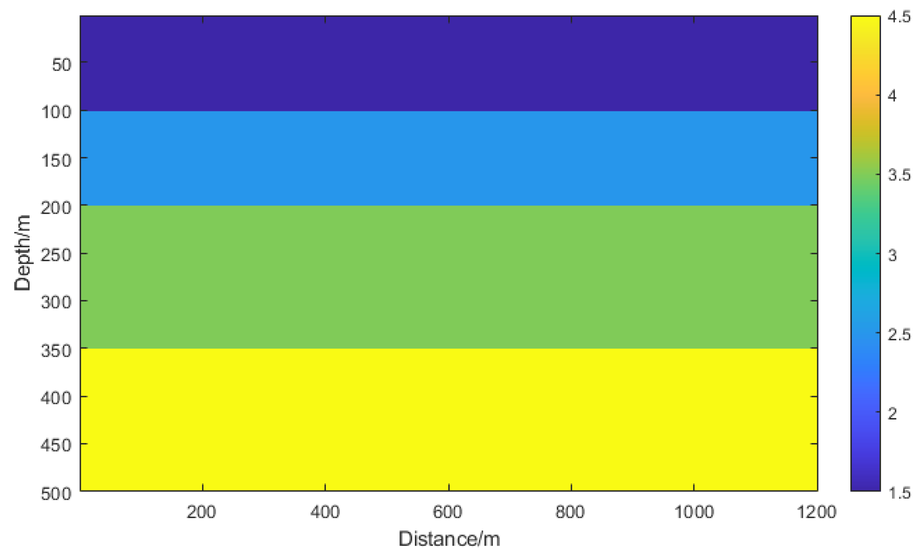
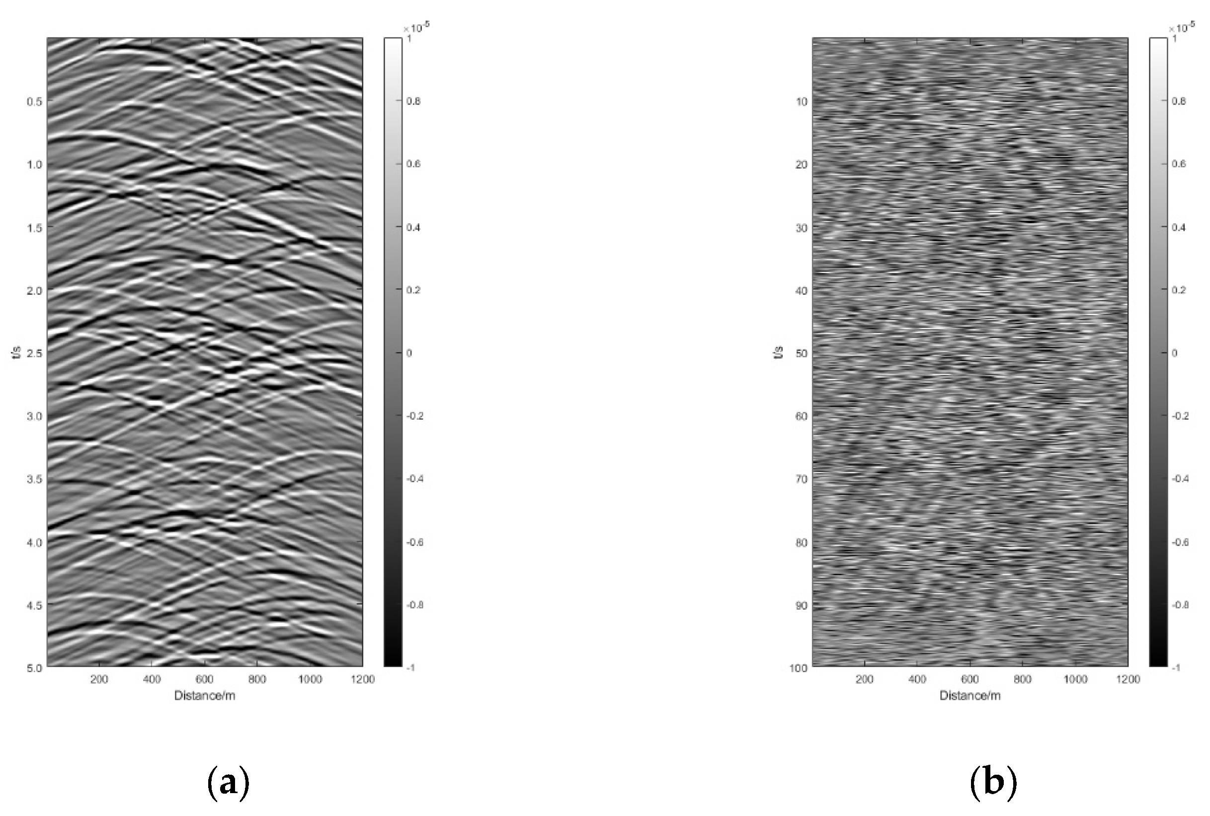
In this paper, we first use a simple and small four-layered model to verify the feasibility of this idea experimentally. The velocity model we used is shown in Figure 1. The random waveforms used are shown in Figure 2.

Figure 1.
Simple-layered model.

Figure 2.
Random passive-source waveform.
We used 2000 randomly distributed subsurface passive sources excited at random time points below 300 m. Once excited, these point sources will vibrate continuously for random periods of time, and the resulting waves are finally received by the geophone. The waveforms are formed by convolution of low-frequency Ricker wavelet with a main frequency of 12 Hz and random sequences. Twelve hertz is just a random value we chose during the experiment to meet the low-frequency range, if necessary, we can also choose a lower or higher center frequency. In general, the smaller the grid spacing and sampling interval, the higher the resolution of the seismic record, so we set a grid spacing of 1 m and a sampling interval of 0.5 ms and recorded continuously for 150 s. The resulting passive seismic records with 5 s and passive seismic records with 100 s are shown in Figure 3.
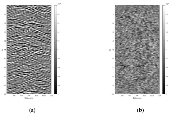
Figure 3.
Short-period passive seismic recording and long-period passive seismic record. (a) Passive seismic records with short periods; (b) passive seismic records with long periods.
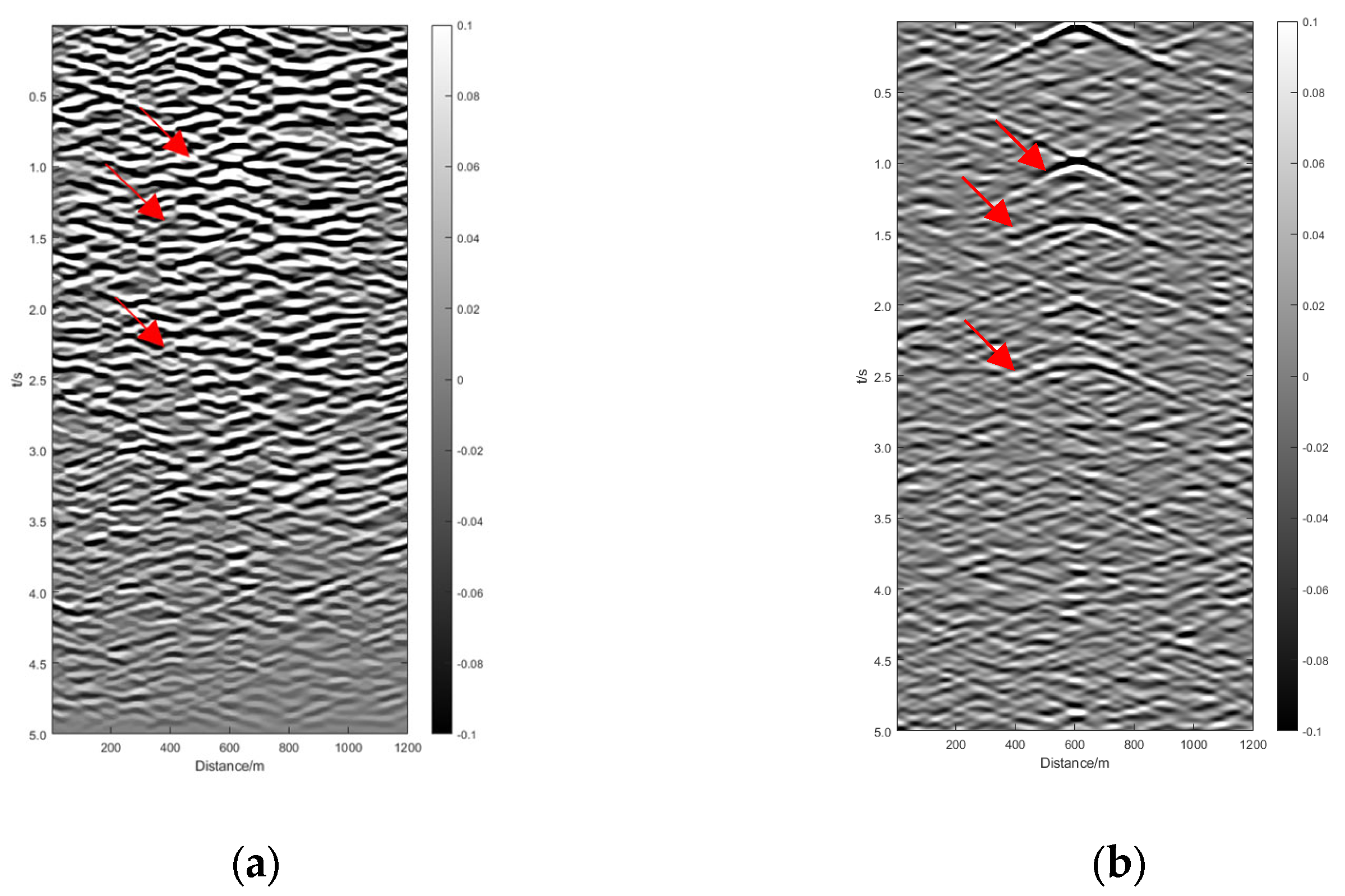
Next, we use the cross-correlation method to reconstruct them, and the resulting reconstructed seismic records are shown in Figure 4. It can be clearly seen that the waveforms of the seismic record with long period are clearer and more continuous, and the intensity of coherent noise is lower. The waveform of the reconstructed seismic record is incomplete, and the weak signal is almost buried in the coherent noise, which will affect the subsequent imaging and inversion if used directly.
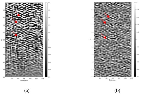
Figure 4.
Reconstruction result of cross-correlation between passive seismic records with short pe-riods and passive seismic records with long periods. (a) The reconstructed result of passive seismic records with short periods; (b) the reconstructed result of passive seismic records with long periods.
From the above results, we know that the reconstruction results of passive seismic records with short periods have lower signal-to-noise ratio, stronger coherent noise, weaker effective signal, and more spurious events compared with the reconstruction results of passive seismic records with long periods. This is due to the fact that we used a large number of noise sources, and they can all continue to vibrate for a period of time, so the quality of the noise in each small period of time is not very different. The longer the recording time is, the more effective signals are received and the better the reconstructed seismic record is.
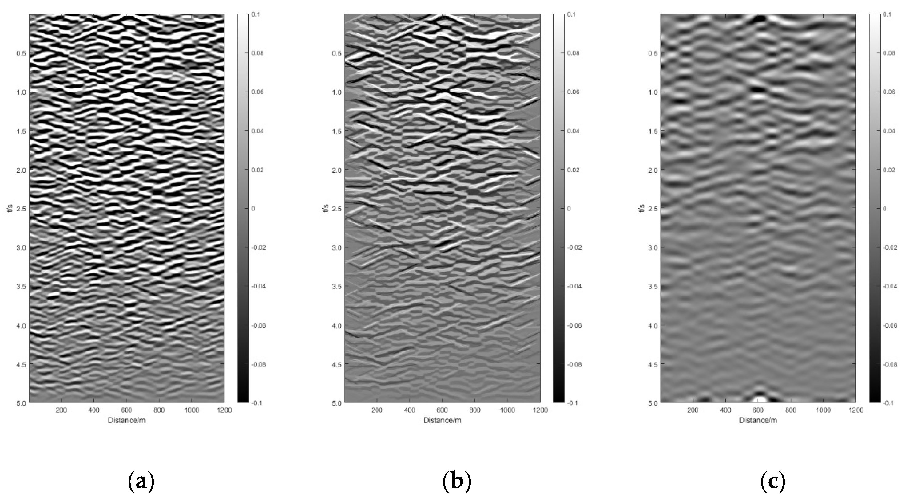
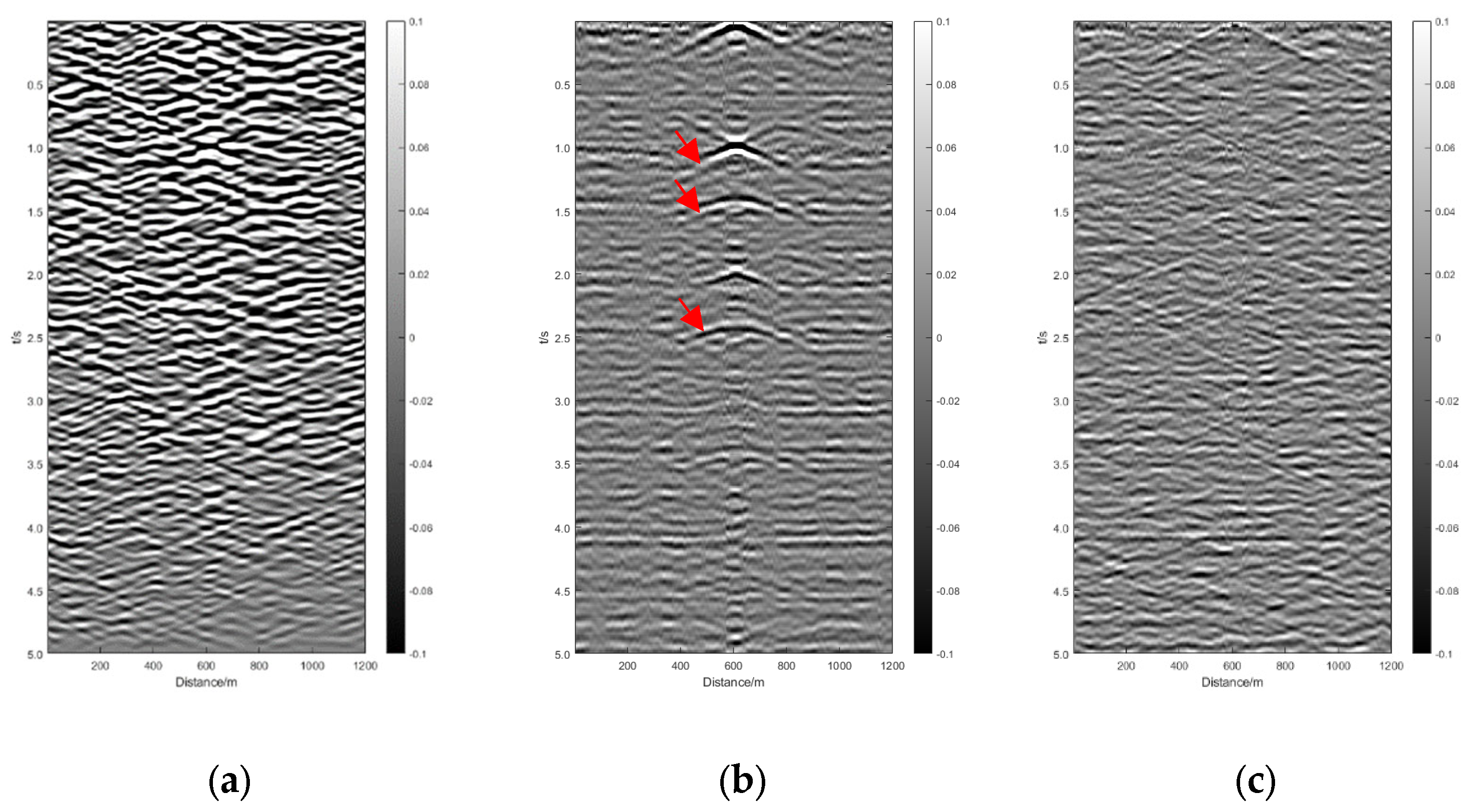
We want to suppress the coherent noise in the reconstruction results of passive seismic records with short periods, so that they have a high signal-to-noise ratio similar to that of the reconstruction results of passive seismic records with short periods. Therefore, we selected two conventional denoising methods for testing. As shown in Figure 5, when it is processed using median filtering, a small filtering window leads to little processing effect, and a large filtering window causes the effective signal to be mixed with the strong coherent signal. When it is processed using f-k filtering, only a small amount of the effective signal is enhanced, and most of the signal becomes weaker. Conventional methods cannot achieve good processing results, so we try to adopt a deep learning approach for testing.
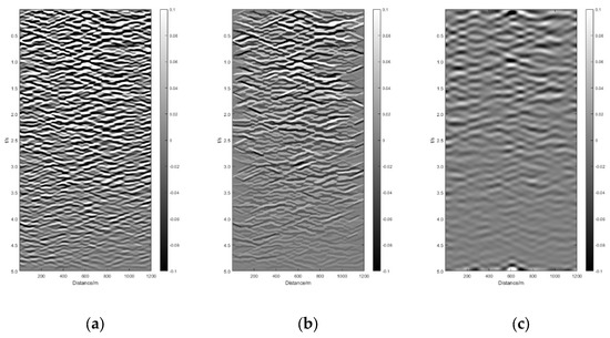
Figure 5.
Two conventional methods process the results. (a) Small filter window median filter pro-cessing result; (b) large filter window median filter processing result; (c) f-k filtering processing re-sult.
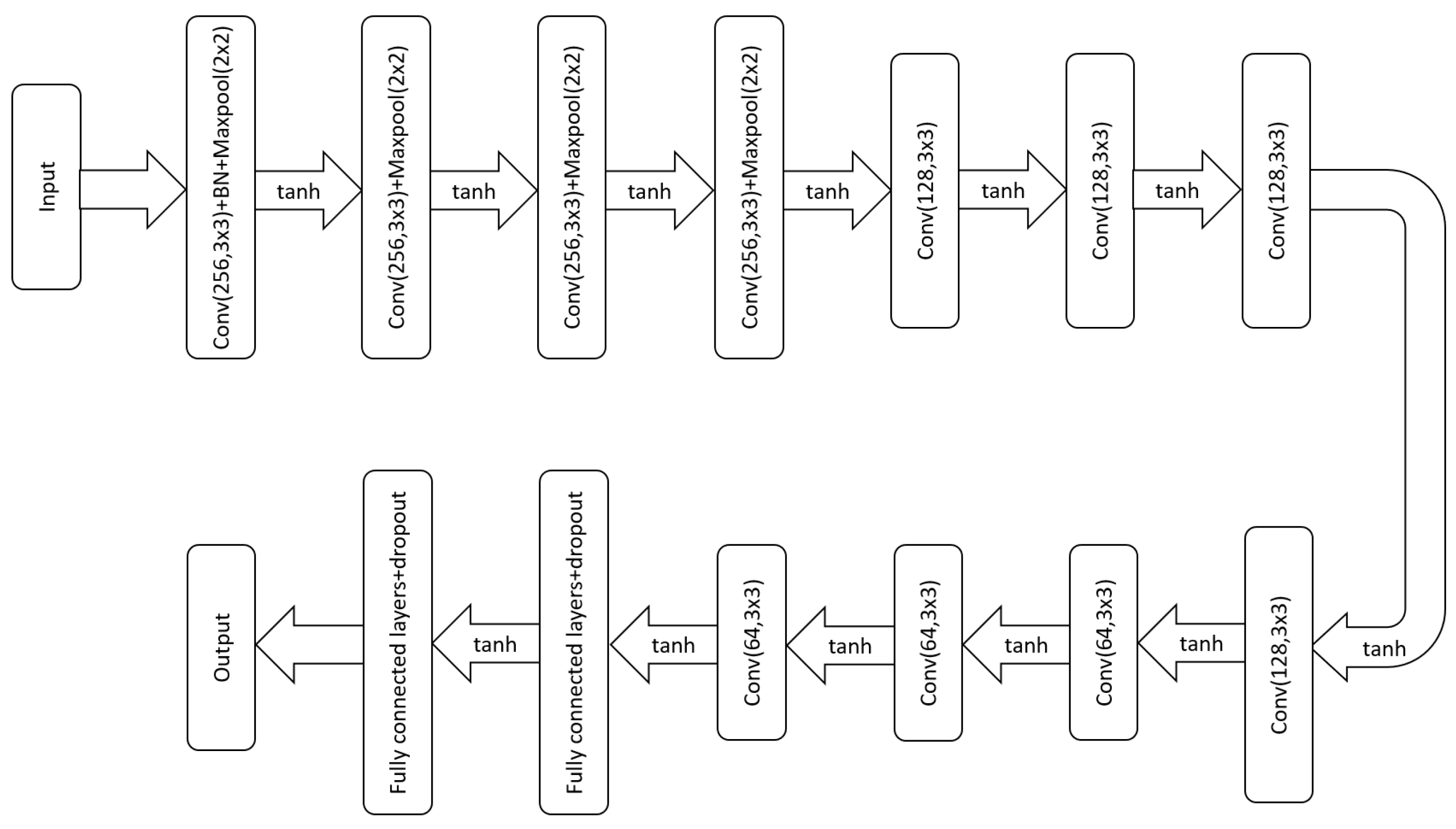
The deep learning network model we used is shown in Figure 6. Although the excitation time and duration of underground sources are random, the virtual shot seismic records of adjacent locations in similar time periods are always similar, so their contribution to the neural network is not large. Therefore, we select seven receiving point positions that are far away from each other and select virtual shot records reconstructed from four segments of noise records with a certain interval for each position as the training set. Additionally, the training labels use the reconstructed results of passive seismic records with long periods of virtual shot locations in corresponding virtual shot locations, respectively; the test set uses the reconstructed results of passive seismic records with short periods of virtual shots reconstructed in other locations different from the training set to test the performance of the completed training network.

Figure 6.
Deep learning network model.
The deep learning framework used in our experiment is tensorflow-gpu, version 1.8. The number of epochs is set to 500, the activation function is tanh, and the dropout is given as 0.6 to prevent overfitting on the one hand and to give more expectation to the potential of the neural network on the other. The optimizers use adam. Among them, the main factors that affect the training time are the size of the dataset and the number of epochs. The training took a total of 8 h, and the processing of the test data took less than 1 min. The result of the test data processed by the neural network and the difference between it and the reconstruction result of the corresponding passive seismic records with long periods are shown in Figure 7.
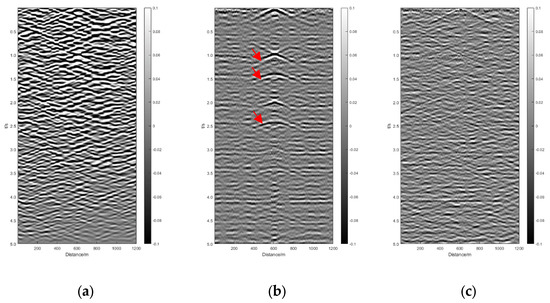
Figure 7.
The result before and after data set processing by the neural network, and the difference between the result and the reconstruction result of passive seismic records with long periods. (a) The reconstructed result of passive seismic records with short periods; (b) the result of the test data processed by the neural network; (c) difference between processing results and the reconstruction result of passive seismic records with long periods.
After comparison, we can find that in the effective signals buried in the reconstruction results, the passive seismic records with short periods are extracted, which effectively improves the signal-to-noise ratio and lays a good foundation for improving the imaging accuracy in the future. Comparing the reconstruction results of passive seismic records with long periods, we can also find that the level of coherent noise is lower in our processed reconstruction record. Observing the difference profile, we can find that the effective waves are effectively extracted, and the difference profile basically contains no information of effective waves. Only the coherent noise interference of the reconstruction record of passive seismic records with long periods and the lateral interference generated during the deep learning processing exist. Therefore, we can confirm that this means of data enhancement reconstruction results of passive seismic records with short periods is feasible and effective. The disadvantage is that some parts of the reflected wave will show weak amplitude, but its partial effect can be attenuated by gain.
3.2. Complex Model Numerical Experiment
From the processing of the simple-layered model, we can see that good results can be obtained by using convolutional neural networks to process reconstructed records of passive seismic records with short periods. Then, is it possible to achieve good results for the processing of complex models?
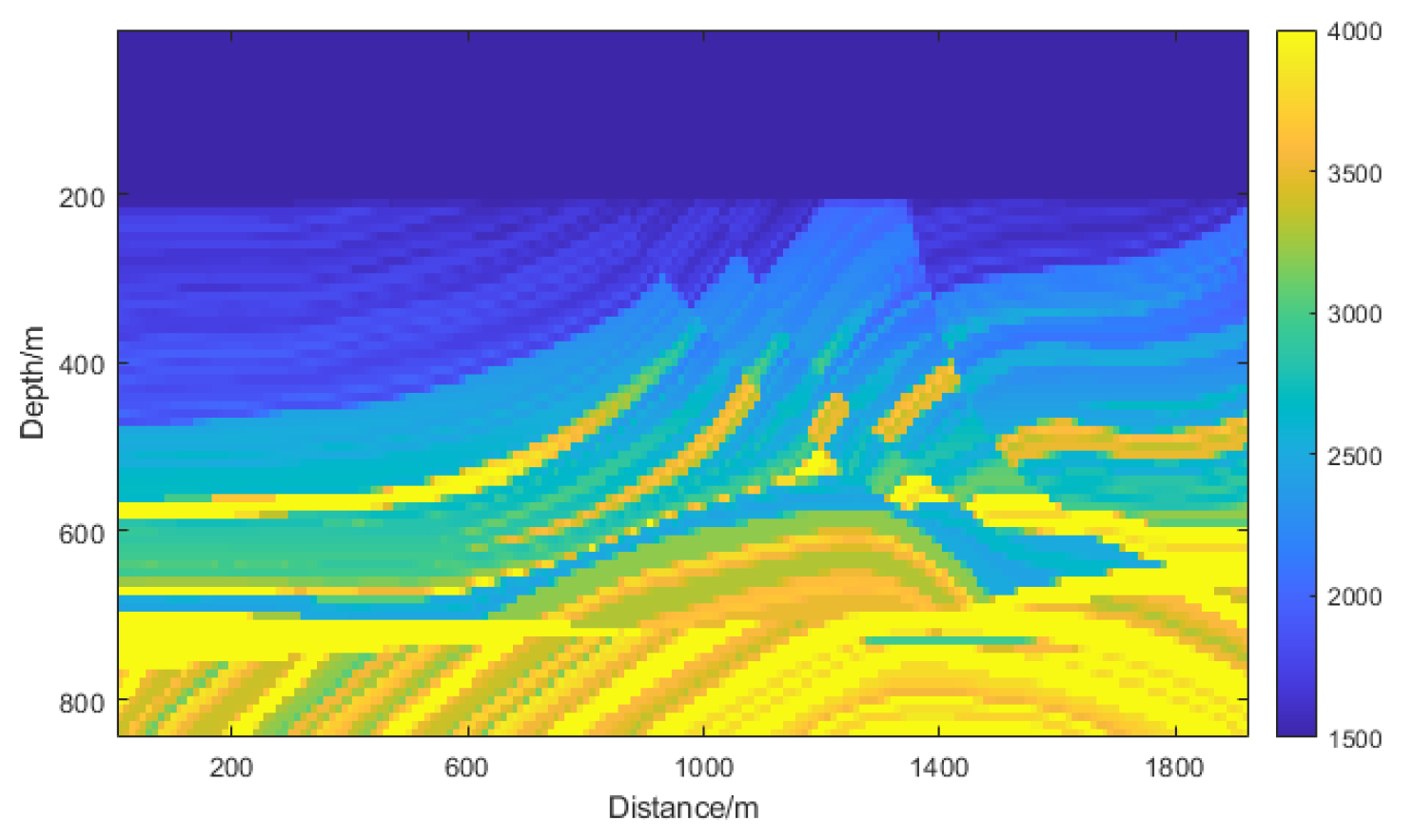
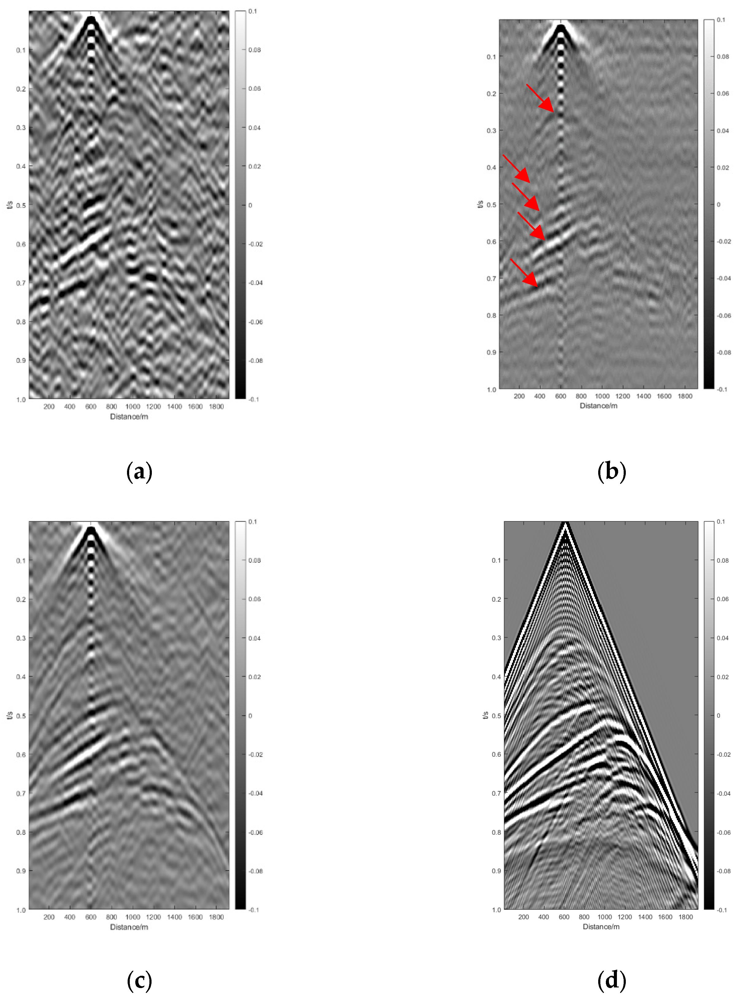
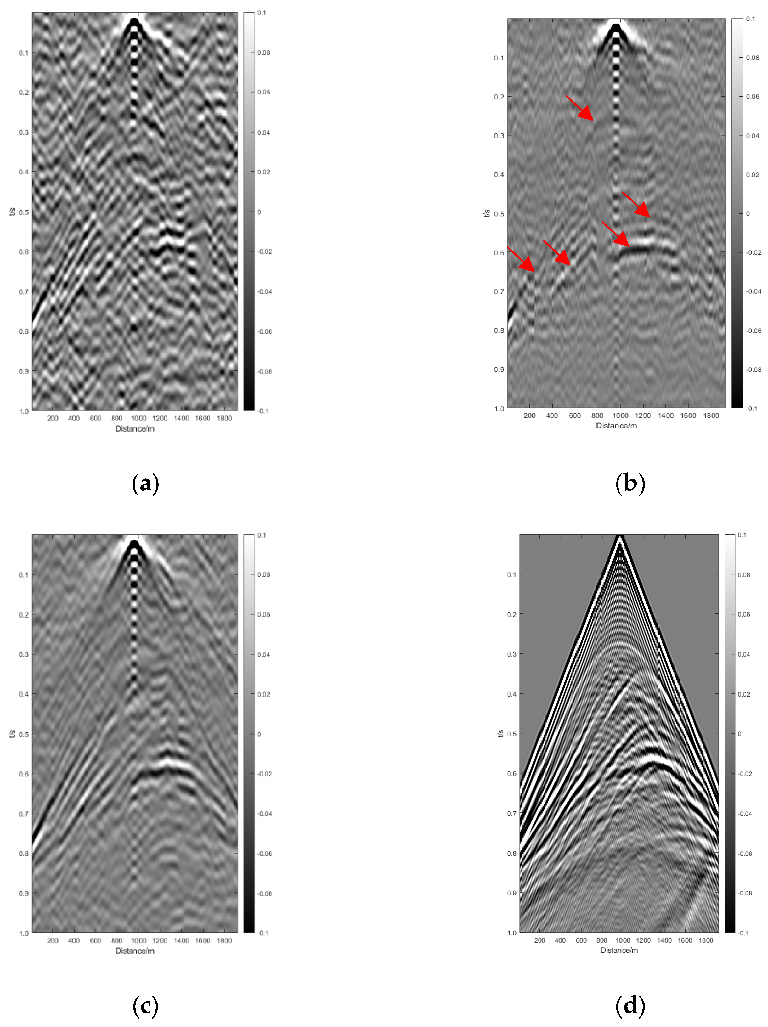
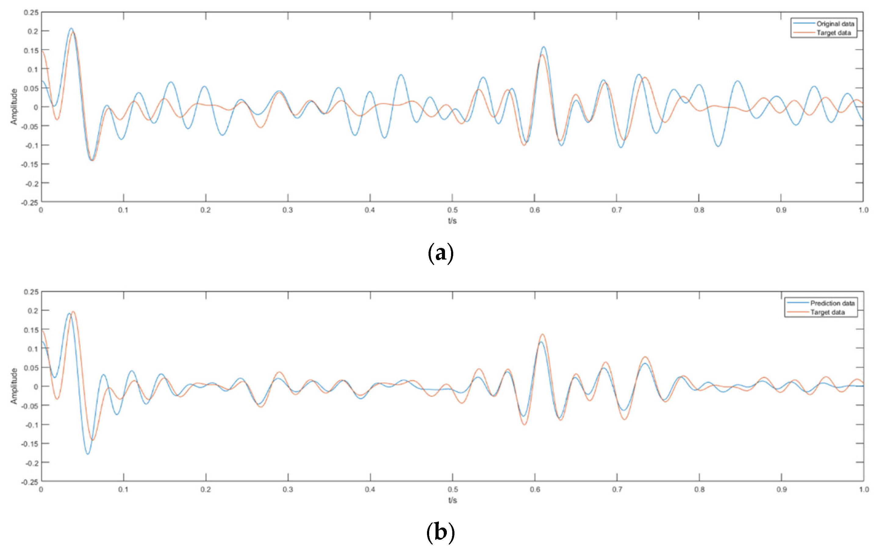
We use a complex velocity model as shown in Figure 8 for our experiments. We use 192 channels for reception, and we randomize the source excitation location and time point in order to realistically simulate the real situation of a passive seismic record in the subsurface. In order to test the effect of the model on different waveforms, a random noise source was used for this test tremor source so that it occasionally appears to be sparser or denser during the recording period. The experimental results are shown in Figure 9 and Figure 10. Here, we select the reconstruction records of passive seismic records with short periods, processing results of passive seismic records with short periods, passive seismic records with long periods, and active-source forward modeling results. The virtual shots located at channel 60 and channel 96, respectively, are for display. In order to facilitate the observation of details, we only capture the reconstruction records of the first 1.0 s, which are rich in waveforms and have a large impact on the subsequent processing for observation and comparison. Figure 11 shows a comparison of the data in one channel when the virtual shot is located in the 60th channel.

Figure 8.
Complex model we used.
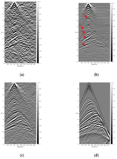
Figure 9.
The 60th trace set effect display. (a) The reconstructed result of passive seismic records with short periods; (b) the result of the test data processed by the neural network; (c) the recon-structed result of passive seismic records with long periods. (d) Active-source forward modeling result.
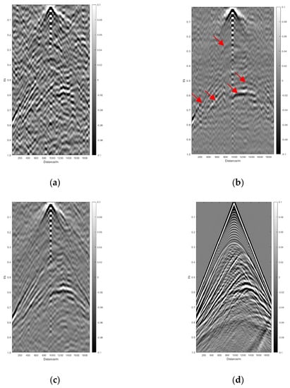
Figure 10.
The 96th trace set effect display. (a) The reconstructed result of passive seismic records with short periods; (b) the result of the test data processed by the neural network; (c) the recon-structed result of passive seismic records with long periods. (d) Active-source forward modeling result.
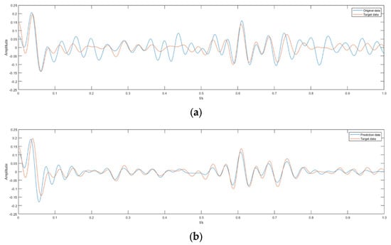
Figure 11.
Comparison of trace waveforms. (a) Single-channel comparison of passive seismic rec-ords with short periods before processing vs. passive seismic records with long periods. (b) Single-channel comparison of passive seismic records with short periods after processing vs. passive seis-mic records with long periods.
By comparison, we can find that the coherent noise, which is originally comparable with the effective signal energy, is well suppressed after processing, and the noise level is even lower than that of reconstruction of passive seismic records with long period, while the weak effective signal is well retained. The spurious events in the recordings are also suppressed effectively. Although there is still a gap between the waveforms in the processed recordings and the active-source recordings, the critical reflected waves are well displayed. Comparing the data of the channels, the processed reconstructed channel set of passive seismic records with short periods cannot only match better with the reconstructed channel set of passive seismic records with long periods in terms of phase, but also, it is closer in terms of amplitude. Generally speaking, the more far away from the surface the coherent noise interferes with the channel set, and our network can suppress it very well. In comparison with the simple laminar model, although the results of our complex model processing are not as highly restored, and the strength and continuity of the effective signals after processing are not as strong as those of the reconstruction records of passive seismic records with long periods, our model still effectively extracts the effective signal and reduces the intensity of the coherent noise, which is even weaker than that of the reconstruction records of passive seismic records with long periods. With this method, enhancement of the effective signal and reduction in the effects caused by coherent noise are guaranteed. Additionally, only a short period of recording time is required to achieve this, significantly reducing the dependence of passive seismic record exploration methods on recording time.
4. Discussion
Method selection of seismic interferometry: There are three common seismic interferometry methods. They are cross-correlation, multidimensional deconvolution, and cross-coherence. Among them, the multidimensional deconvolution method and cross- coherence method have certain effects on the suppression of multiple and surface waves, although they are clearer in waveform display. However, the cross-correlation method also has the advantages of a simple formula, small calculation, and stable effect. For this experiment, it is possible to choose which seismic interferometry method to make the dataset with. We chose the cross-correlation method just to obtain the dataset faster and more stably.
Selection of neural network framework: For the experiment of enhancing the weak signal of passive seismic records with short periods, we only used the most traditional convolutional neural network and achieved good results. Maybe there will be more suitable and effective convolutional neural networks in the future, and we will keep trying this.
Setting of hyperparameters: It is widely known that the hyperparameters of a convolutional neural network include the number of convolutional layers, the number of convolutional kernels contained in each layer, the learning rate, dropout, etc. When the number of convolutional layers is small, the model cannot learn enough features, and too many will lead to slow learning but little improvement. The number of convolutional kernels per layer depends on the computing hardware and the size of the input and output. Too small a learning rate leads to slow learning and overfitting, too large will lead to loss shock and nonconvergence. Too small a dropout leads to overfitting, and too large a dropout leads to underfitting. Epoch is the opposite of dropout, too small leads to underfitting, and too large leads to overfitting. Too small a batch size leads to wasted memory and reduced efficiency, too large leads to convergence of the model to some local extrema. After many attempts, the hyperparameters in this paper are reasonable and finally achieve good results.
In this paper, we propose a deep-learning-based method for weak signal recognition and coherent noise suppression of passive seismic records with short periods. Using reconstructed records of passive seismic records with long periods as the label and reconstructed records of short-period passive seismic records as the training set, the obtained network has a good noise reduction and signal recognition capability. After using this network for reconstruction records of passive seismic records with short periods, the processing results have a high signal-to-noise ratio. It makes the shorter records of conventional passive seismic records available, which greatly improves the utilization of passive seismic records and can effectively reduce the recording time required for acquisition and improve acquisition efficiency.
In addition, the method can be used for real-time monitoring of the quality of passive seismic exploration because it can extract effective signals for passive seismic records with short periods, and we can avoid the situation where the passive sources are collected in areas where the subsurface seismic sources are not abundant, or where the data are not available due to the short reception time of the instrument. It also has some application value for construction, earthquake monitoring, groundwater flow, dam structure monitoring, and other work that requires continuous real-time monitoring of subsurface tectonic changes.
Author Contributions
Methodology and manuscript writing B.Z.; project administration and review, L.H.; experiments design guidance and review, P.Z.; investigation and validation, Y.Y. All authors have read and agreed to the published version of the manuscript.
Funding
This research was funded by the National Natural Science Foundation of China, grant numbers 42130805, 42074151 and 42004106, the Natural Science Foundation of Jilin Province (No. YDZJ202101ZYTS020), and the Lift Project for Young Science and Technology Talents of Jilin Province (No. QT202116).
Data Availability Statement
The data presented in this study are available on request from the corresponding author.
Conflicts of Interest
The authors declare no conflict of interest.
References
- Draganov, D.; Wapenaar, K.; Mulder, W.; Singer, J.; Verdel, A. Retrieval of reflections from seismic background-noise measurements. Geophys. Res. Lett. 2007, 34, 4305-1–4305-4. [Google Scholar] [CrossRef]
- Wapenaar, K.; van der Neut, J.; Ruigrok, E. Passive seismic interferometry by multidimensional deconvolution. Geophysics 2008, 73, A51–A56. [Google Scholar] [CrossRef][Green Version]
- van Groenestijn, G.J.; Verschuur, D.J. Estimation of primaries by sparse inversion from passive seismic data. Geophysics 2010, 75, SA61–SA69. [Google Scholar] [CrossRef][Green Version]
- Ruigrok, E. Receiver-pair seismic interferometry applied to body-wave USArray data. Geophys. J. Int. 2014, 198, 895–905. [Google Scholar] [CrossRef][Green Version]
- Wapenaar, K. Retrieving the elastodynamic Green's function of an arbitrary inhomogeneous medium by cross correlation. Phys. Rev. Lett. 2004, 93, 254301. [Google Scholar] [CrossRef] [PubMed]
- LeCun, Y.; Bottou, L.; Bengio, Y.; Haffner, P. Gradient-based learning applied to document recognition. Proc. IEEE 1998, 86, 2278–2324. [Google Scholar] [CrossRef]
- Hinton, G.E.; Salakhutdinov, R.R. Reducing the Dimensionality of Data with Neural Networks. Science 2006, 313, 504–507. [Google Scholar] [CrossRef] [PubMed]
- Zhang, K.; Zuo, W.; Chen, Y.; Meng, D.; Zhang, L. Beyond a Gaussian Denoiser: Residual Learning of Deep CNN for Image Denoising. IEEE Trans. Image Process. 2017, 26, 3142–3155. [Google Scholar] [CrossRef] [PubMed]
- Zhu, W.; Beroza, G.C. PhaseNet: A deep-neural-network-based seismic arrival-time picking method. Geophys. J. Int. 2019, 216, 261–273. [Google Scholar] [CrossRef]
- Ross, Z.E.; Meier, M.A.; Hauksson, E.P. Wave arrival picking and first-motion polarity determination with deep learning. J. Geophys. Res. Solid Earth 2018, 123, 5120–5129. [Google Scholar] [CrossRef]
- Sun, J.; Slang, S.; Elboth, T.; Greiner, T.L.; McDonald, S.; Gelius, L.-J. A convolutional neural network approach to deblending seismic data. Geophysics 2020, 85, WA13–WA26. [Google Scholar] [CrossRef]
- Tschannen, V.; Delescluse, M.; Ettrich, N.; Keuper, J. Extracting horizon surfaces from 3D seismic data using deep learning. Geophysics 2020, 85, N17–N26. [Google Scholar] [CrossRef]
- Song, H.; Mao, W.; Tang, H. Application of deep neural networks for multiples atte-nuation. Chin. J. Geophys. 2021, 64, 2795–2808. [Google Scholar]
- Petrov, S.; Mukerji, T.; Zhang, X.; Yan, X. Shape Carving Methods of Geologic Body Interpretation from Seismic Data Based on Deep Learning. Remote Sens. 2022, 15, 1064. [Google Scholar] [CrossRef]
- Wapenaar, K. Green's function retrieval by cross-correlation in case of one-sided illumination. Geophys. Res. Lett. 2006, 33, 19304-1–19304-6. [Google Scholar] [CrossRef]
- Wapenaar, K.; van der Neut, J.; Ruigrok, E.; Draganov, D.; Hunziker, J.; Slob, E.; Thorbecke, J.; Snieder, R. Seismic interferometry by crosscorrelation and by multidimensional deconvolution: A systematic comparison. Geophys. J. Int. 2011, 2011 185, 1335–1364. [Google Scholar] [CrossRef]
- Thorbecke, J.W.; Draganov, D. Finite-difference modeling experiments for seismic interferometry. Geophysics 2011, 76, H1–H18. [Google Scholar] [CrossRef]
Publisher’s Note: MDPI stays neutral with regard to jurisdictional claims in published maps and institutional affiliations. |
© 2022 by the authors. Licensee MDPI, Basel, Switzerland. This article is an open access article distributed under the terms and conditions of the Creative Commons Attribution (CC BY) license (https://creativecommons.org/licenses/by/4.0/).

