Abstract
The received signal of passive radar based on mobile communication signals contains direct and multipath interference (DMI) signals from multiple co-channel base stations (CCBS). The direct signal spatial spectrum of each CCBS should be obtained first to eliminate the co-channel interference. The performance of the traditional spatial spectrum estimation algorithms based on uniform linear array (ULA) is related to the number of array elements. In the complex co-channel interference environment, the array requires an ultra-large number of array elements and the spatial spectrum estimation resolution is poor. This paper proposes a method for estimating the direct signal spatial spectrum of the CCBS by fusing coprime array and compressive sensing. Firstly, an augmented virtual array signal is constructed by using the second-order statistics of the received signals of the coprime array and then the compressive sensing algorithm is used to estimate the spatial spectrum of the direct signal of the CCBS. The proposed method can achieve higher resolution and higher-degrees-of-freedom (DOFs) performance than traditional ULA by using the same number of array elements. The effectiveness of the proposed method is verified by numerical simulation analysis and experimental data.
1. Introduction
Passive radars with no transmitter exploit existing third-party non-cooperative emitters to detect, locate and track targets [1,2]. Compared to active radar, passive radar has the advantages of better covertness, no required spectrum allocation, a simple structure and easier radar networking [3,4]. At present, the available third-party illuminators of opportunity (IoO) mainly include frequency modulation (FM) broadcast signal [5,6], digital audio/video broadcast (DAB/DVB) [6,7,8], WiFi [9] and mobile communication systems (Global System for Mobile Communication, Long-Term Evolution, 5G) [10,11,12,13,14,15], etc. Compared with traditional low-frequency-band IoO, such as FM/DVB-T, using mobile IoO communication signals has the following advantages: (1) Benefiting from the dense distribution of mobile communication base stations, it provides a foundation for radar networking and it is easy to achieve multi-station integration and improve the positioning accuracy and detection ability of the target [16,17]. (2) Mobile communication signals have a higher frequency and larger spectral bandwidth, which provides a higher range and higher speed resolution for radar use [18,19,20]. Therefore, it has become a hot research field in PBR [10,11,12,13,14,15,16,17,18,19,20,21,22].
Using mobile communication signals as an IoO brings benefits, but also increases the complexity of radar system signal processing. In traditional low-frequency-band irradiation sources for passive radar, such as FM and analog TV signals, the transmitters are sparsely distributed and the frequency division multiple-access (FDMA) transmission technology is adopted. The transmitters sharing the same frequency are far apart [17]. Therefore, the interference signals mainly come from the direct signal of the base station that is used as the illuminator opportunity (BS-IoO) [23] and the co-channel interference is usually ignored [24]. Unlike the traditional low-frequency-band irradiation sources used as the IoO, the mobile communication base stations adopt the dense cellular distribution and some of them share the same frequency band. As a result, the signals received by the radar systems cannot be filtered in the frequency domain to eliminate the DMI of the co-channel. Therefore, the signal received by the passive radar system uses the mobile communication signal, as the IoO contains both the DMI from the BS-IoO and other CCBSs [25,26]. Because the energy of the co-channel interference is much greater than that of the target echo, the target echo is masked in the co-channel interference clutter [27]. Though the energy of the target can be improved through coherent integration, the targets will still be covered up by the sidelobes of the clutter, causing miss detection. Therefore, the co-channel interference clutter in the received signal must be eliminated to effectively detect the target [28].
The signals transmitted by each mobile communication base station are different; the direct reference signal obtained from the beamforming in the direction of the BS-IoO can only be used to eliminate the DMI from the BS-IoO in the echo channel, it cannot be used to eliminate the DMI from the CCBSs [29]. Therefore, it is necessary to obtain the transmitted signals of each CCBS as a reference signal to eliminate the interference clutter.
The premise of obtaining the reference signals from each CCBS is to obtain the direct signal spatial spectrum information of CCBS. In this paper, the signal with the strongest energy reaching the receiving antenna from each CCBS is called the direct signal. In [30], the subspace method is used to obtain the direct signal direction of arriving (DOA) of the BS-IoO, which can be used when the amount of co-channel interference is small, but a large-scale array antenna is required in a complex co-channel interference environment; otherwise, it will fail. In [29], the m-Capon spectrum estimation method is used for the target signal, co-channel interference signal and direct signal. This method still maintains a high angular resolution when the number of snapshots is small and can perform spatial spectrum estimation for a certain number of strong co-channel interference signals. However, this method also has shortcomings. Due to the limitation of the number of array antennas in the actual system, only a limited number of DOAs with strong co-channel interference can be estimated and the estimation effect is not complete. In [17], the DOA estimation of direct signal is realized using a ULA array. Due to the limitation of the array size, only the DOAs of a few strong direct signals from the CCBS can be estimated each time. This method can only obtain sufficient cancellation performance with a small amount of co-channel interference, but when the amount of co-channel interference is large, it is limited by the actual number of array antennas. This will lead to a deterioration in the accuracy of the spatial spectrum estimation each time and the spatial spectrum estimation of the co-channel interference signals needs to be repeated many times, which will undoubtedly increase the complexity in the system calculation. In [31], a method similar to that of the study in [17] is used to realize the DOA estimation of direct signal from the CCBSs and the spatial spectrum estimation performance is limited by the array size in a complex co-channel interference environment. Therefore, due to the dense distribution of mobile communication base stations, the signals received by the radar system include DMI from multiple CCBSs, resulting in a large amount of interference. The spatial spectrum estimation method under the traditional uniform linear array (MUSIC, Capon, Maximum likelihood, etc.) has a poor resolution in the complex co-channel interference environment and will fail when the amount of interference is greater than the number of array elements [17]. If the traditional spatial spectrum estimation method is applied to it, larger array size is required, which leads to a great increase in the complexity of the system.
Aiming at this problem, this paper proposes a method for estimating the direct signal spatial spectrum from the CCBSs by fusing coprime array and compressive sensing algorithm. Firstly, the signal receiving model of the radar in a complex co-channel interference environment is constructed. Then, using the second-order statistics of signals received by the coprime array, the enhanced virtual array signal is constructed, which effectively breaks through the actual array size in the traditional ULA [32]. On this basis, the compressed sensing algorithm is used to achieve a high-resolution estimation of the direct signal spatial spectrum of the CCBSs. Through simulation analysis, the proposed method is better than MUSIC, Capon, maximum likelihood (MLE) and compressed sensing (CS) spatial spectrum estimation methods based on ULA in the spatial spectrum estimation performance of CCBS strong direct signals in a complex co-channel interference environment. The experimental data verify that the proposed algorithm can be applied in practical scenarios.
2. Materials and Methods
2.1. Signal Model
The layout of the mobile-communication-based PBR is shown in Figure 1, where β is the bistatic angle of the radar and α is the angle between the radar line of sight and the target. Using a coprime array antenna with L array elements as the receiving antenna of the passive radar, the received signal of each array element can be expressed as:
where represents the envelope of the -th moving target echo signal, is the complex envelope of the -th co-channel interference signal from the -th CCBS (where we assume that is the BS-IoO, the rest are the CCBSs), is the noise signal of the -th array element and is the distance from the -th array element to the reference array element.
Figure 1.
Schematic diagram of radar target detection structure for mobile communication passive radar.
is the DOA of the -th moving target echo and is the DOA of the -th co-channel interference signal from the -th CCBS. is the wavelength of the irradiation source signal.
is the total number of target echoes, is the number of CCBSs and is the -th CCBS that has co-channel interference in total.
As shown in Equation (1), the interferences in the surveillance channel of passive radar based on mobile communication include the interferences from both BS-IoO and CCBSs. This is different from the conventional low-frequency-band PBR, in which only the interference clutter from the BS-IoO is considered. To eliminate the co-channel interference, the spatial spectrum of the direct signal of the CCBSs should be known and then the reference signals from the CCBSs are obtained through beamforming. It is necessary to improve the traditional passive radar processing (as seen in Figure 2). First, the spatial spectrum of the received signal is estimated in the reference channel to obtain the DOAs of the CCBSs. Then, the reference signals of the CCBSs are obtained by beamforming and the co-channel interference in the echo channel is eliminated by the cancellation method. The improved signal processing of the passive radar based on mobile communication is shown in Figure 3.
Figure 2.
Traditional passive radar signal processing process.
Figure 3.
Signal processing process of passive radar for mobile communication.
Considering that the energy of the DMI from BS-IoO or CCBSs is higher than that of the target echo, the target echo is treated as noise in Equation (1) in the co-channel interference spatial spectrum estimation [28]. The co-channel interference is prioritized to estimate the spatial spectrum, so we assume that the interference from both the BS-IoO and CCBSs are regarded as co-channel interference, whereby the received signal can be expressed as:
where:
The received signal is expressed in vector form as:
where represents the number of co-channel interferences, the array steering vector corresponding to the -th co-channel interference is expressed as , represents dimension coprime array manifold matrix, the co-channel interference waveform vector is expressed as , is the noise vector. denotes the transpose of the vector.
2.2. Direct Signal Spatial Spectrum Estimation Algorithm Based on the Fusion of Coprime Array and Compressed Sensing
To realize co-channel interference spatial spectrum estimation and interference suppression in a complex interference environment, the coprime array is used as the receiving array. A direct signal spatial spectrum estimation method using coprime array and compressed sensing is proposed (as seen in Figure 3). The sparse array architecture of coprime array can break through the limitation of Nyquist sampling rate and realize under-sampling and sparse perception of incident signals. An augmented virtual array is formed on the virtual domain by calculating the difference coarray of the coprime array and the performance of the array in degrees of freedom and resolution is improved. Further, virtual domain signal fusion compressed sensing sparse reconstruction algorithm is used to achieve high-resolution estimation of co-channel direct signal in complex co-channel interference environment.
A typical structure of coprime array can be seen in Figure 4, which consists of two uniform linear subarrays whose number of elements is mutually prime. The number and spacing of the first ULA array elements are and , respectively. The number and spacing of the first ULA array elements are and , respectively. is set to half wavelength, denoted as . The total number of elements in the coprime array is and the positions of the physical array elements are:
Figure 4.
Extended coprime array construction.
The structure of the extended coprime array is described above. The structure of the coprime array has many styles. For example, the simple coprime array is to change the number of elements of the subarray from to and the other configurations remain unchanged. The configuration will reduce the utilization rate of the array elements. The method in this paper uses the extended coprime array and the measured data verification part adopts a simple coprime array due to hardware conditions.
The elements in the virtual array are acquired by the covariance statistic of the received signal. Each value in the covariance matrix can represent the equivalent received signal of a virtual array element. Thereby, a virtual received signal of an extended virtual array can be formed and the spatial spectrum estimation can be realized by using the virtual domain signal. The covariance statistic of the received signal can be expressed as:
where represents the -th co-channel interference power, is the steering vector of the -th co-channel interference, is the covariance matrix of co-channel interference, represents noise power and represents the dimensional unit matrix. denotes the statistical expectation operator and denotes the conjugate transpose of a matrix or vector. In practice, we use sample averaging, as in Equation (6).
The covariance matrix is composed as shown in Formula (7):
As can be seen from Formula (7), the elements of the -th row and the -th column in the covariance matrix of the coprime array are expressed as:
where , represents a conjugate operation. It can be seen from the above formula that the correlation statistic operation of the received signals of the -th and -th array elements in the array is expressed as the difference set of the physical array element positions in the exponential term. It is similar to the steering vector . The exponential function term in the second-order statistic can be regarded as the steering vector of an equivalent virtual array and the position of each array element in the virtual array as:
can be represented by the following four subsets:
where
and correspond to the autocorrelation statistics of the received signals of subarray 1 and subarray 2, respectively, and correspond to the cross-correlation statistics of the received signals of the two sub-arrays, which are mirror images of each other. It can be seen from the above expression that the virtual array element positions and corresponding to the autocorrelation statistics are subsets of and . After the redundancy is removed from , the difference coarray of the coprime array is expressed as
Correspondingly, the equivalent virtual signal corresponding to the virtual array can be obtained by vectorizing the covariance matrix of the coprime array, that is, stacking the columns in the matrix in turn to form a vector, which can be expressed as:
where denotes the vectorization operator that stacks the column vectors of a matrix one by one, so according to Equation (13)
where is an arbitrary vector, represents Kronecker product and represents a conjugate operation. The first part in Equation (12) can be simplified as:
where is the steering matrix of the virtual array, , . Therefore, Equation (12) can be expressed as:
We observe the mathematical model of , which is similar to the original received signal model in Equation (3), whereby the vector can be seen as the equivalent received signal of the virtual array with the corresponding steering matrix . Using the definition of the Kronecker product, it can be known that the process of calculating corresponds to the operation process of the actual array element position difference set . The dimension of is and the dimension of the original array manifold is ; therefore, the virtual array greatly improves the array aperture and DOF to the actual physical array.
We use the extended coprime array with in the simulation analysis in Section 3.2 as an example, as shown in the schematic diagram in Figure 5.
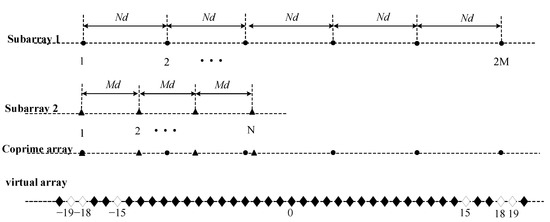
Figure 5.
Schematic diagram of the extended coprime matrix combined with
.
It can be seen from Figure 5 that the obtained virtual array is not continuous and the positions ±15, ±18 and ±19 are holes, so these positions do not have corresponding virtual array elements. Therefore, is not a signal received by a continuous virtual array and there are locations where virtual array elements are missing. However, there is a virtual uniform linear subarray composed of virtual array elements from to positions in the virtual array.
By intercepting the segment of the uniform linear subarray in the non-uniform virtual array, the equivalent virtual signal of the virtual uniform linear array can be obtained by selecting the element at the corresponding position in :
The model can be represented as:
In Equation (18), is the dimensional matrix of each steering vector corresponding to the co-channel interference signal and is like a single snapshot signal vector received by virtual linear array elements. It can be seen that continuous virtual array elements can be obtained only by actual array elements, which improves the DOF of the array.
From Equation (18), it can be considered that is a linear combination of co-channel interference signals from their respective directions. Therefore, the compressed sensing algorithm can be used to solve the DOAs of the co-channel interference and the azimuth angle of is sparsely reconstructed by the sparse reconstruction method in the literature [33] to obtain the spatial spectrum of the co-channel interference. The specific method is to solve the following -norm minimum optimization problem:
where is the energy amplitude vector in all directions of the co-channel interference to be solved, is the 1 norm of and is a constant.
is the observation matrix, which consists of steering vectors in all directions. The observation matrix can be expressed as Formula (20):
is to divide the spatial azimuth angle of into grids to construct a complete spatial grid point, so that the co-channel interference is sparsely distributed in the spatial domain of interest.
In the minimum optimization process of solving Equation (19), the greater the energy of the co-channel interference, the greater the weight it occupies in the minimum optimization process and the high-energy co-channel interference signals will be preferentially reconstructed. Therefore, Equation (19) can be used to estimate the spatial spectrum of strong co-channel interference.
The method from the study of [33] requires that the parameters are real numbers, but the vector parameters in Equation (19) are complex numbers, so they need to be converted into a real-valued domain.
where:
means taking the real part of matrix and means taking the imaginary part of matrix .
Solving for requires the introduction of a new unknown real vector , and are real and imaginary parts of the .
According to the interior point method [33], the optimization problem constrained in Equation (19) can be transformed into the following optimization problem without constraints:
where:
is a scalar. The convex optimization problem in Equation (22) can be solved by Newton’s method [33], which is the solution of Equation (21).
By solving Equation (22), we can obtain , which is a -dimensional vector, which represents the energy amplitude of the interference signal in all directions in the observation matrix . By performing energy detection in all directions, the DOAs of the interference are obtained.
3. Results and Analysis
3.1. Numerical Simulation Description
In this section, the proposed method is simulated and analyzed. The simulation parameters are set according to the mobile communication signal parameters in the actual environment. The simulation scenario is shown in Figure 1.
Mobile communication base stations are located in urban or suburban areas and their coverage radius is 0.3–1 km. In the simulation, the radar receiving antenna is set to be 1 km away from BS-IoO and the CCBSs are distributed about 5 km away from the BS-IoO (meeting the condition that the co-channel interference energy is less than 12 dB relative to the BS-IoO [34]). The radar adopts combined coprime array receiving antennas, with a total of nine omnidirectional array elements (as seen in Figure 5). As a comparison, a ULA antenna with the same number of coprime arrays is selected and the element spacing is half the wavelength.
In the following simulations, we assume that each CCBS has one direct and five multipath signals and there are six interferences in total. In each simulation, the direct signal energy is randomly selected between 20 and 25 dB. The multipath interference energy is randomly selected between 0 and 5 dB, the DOAs of all co-channel interference are randomly selected at [−90° and 90°] and the spatial grid division angle interval is 1°. The above parameters are randomly selected in each Monte Carlo simulation. In the following simulations, the number of CCBSs and specific parameters of co-channel interference clutter are set according to each simulation scenario. We assume that in the simulations, the difference between the sparsely reconstructed DOA of the co-channel interference and its real DOA is no more than 3 dB half-beam width. That is, when the difference between the real DOA and the sparsely reconstructed DOA does not exceed 3°, we think that the correct high-resolution detection and DOA estimation are achieved. Probability of discrimination success = number of successful discrimination/number of Monte Carlo experiments.
3.2. Simulation Results and Analysis
3.2.1. Performance Analysis of DOF
For the DOF simulation when there is too much co-channel interference, eight CCBSs are set, each CCBS has 1 direct signal and 5 multipath interferences and there are a total of 48 co-channel interferences. The energies of direct signal and multipath interference are randomly selected between 20 and 25 dB and 0 and 5 dB, respectively, and their DOAs are randomly selected between [−90° and 90°]. The simulation results are shown in Figure 6.
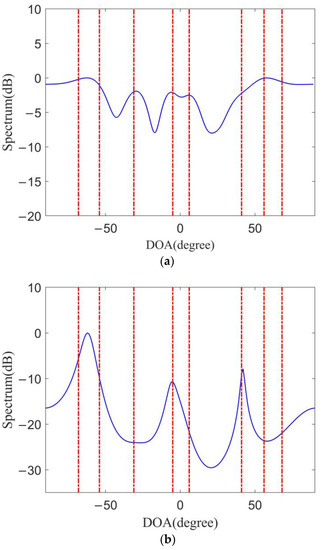
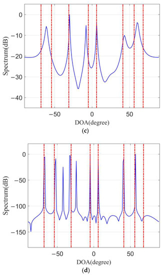
Figure 6.
Co-channel interference spatial spectrum estimation, (a) Maximum likelihood, (b) MUSIC, (c) Compressed sensing based on ULA, (d) the proposed method.
Figure 6 shows that the traditional maximum likelihood and MUSIC algorithms based on ULA almost fail in the case of complex co-channel interference in Figure 6a,b. The compressed sensing (CS) algorithm based on ULA can correctly estimate the DOA of four direct signals of the co-channel, but the peak response is not sharp, as shown in Figure 6c. Therefore, this method cannot effectively estimate the spatial spectrum of co-channel interference in such a complex co-channel interference environment. The proposed method can estimate the DOAs of the direct signal of seven CCBSs, as shown in Figure 6d. From Figure 6d, it can be seen that there is one co-channel direct signal that has not been estimated. The reason is that, in order to simulate the actual environment as much as possible, the direct signal energy of each CCBS is set to be random. The energy of the non-correctly estimated direct signal is lower than that of other signals. Therefore, in order to correctly estimate the DOA of all direct signals, we use a cascade cancellation method in the actual processing process. Firstly, the DOAs of the strongest direct signal are estimated and cancelled and then the echo signal of other sub-strong energies is estimated. For more details about the cascading cancellation algorithm, see Section 3.3 of Field Experiment Results and Analysis.
From Figure 6d, it also can be seen that there are two spurious signals. The reason for these two spurious signals is that in the simulation, the DOAs of the interfering signal are random and there is some low-energy multipath interference gathered in these two azimuths, causing energy accumulation. In the process of sparse reconstruction, they are regarded as two strong direct signals of the co-channel. In the subsequent clutter elimination process, the two spurious signals can be eliminated without affecting target detection. Therefore, in the complex co-channel interference environment, the spatial spectrum estimation performance of the coprime array is obviously better than that of the ULA.
3.2.2. Performance Analysis of Direct-Signal High-Resolution DOA Estimation
In the suburban application environment, when the direct signal of two CCBSs have similar DOAs, it is used to verify the high-resolution performance of the proposed method. For set 2 CCBSs, the direct signal energy of the CCBS is 23 dB and 25 dB, respectively. The first direct-signal DOA is kept at 20° and the second DOA is between 20.5° and 40°, varying from 20.5° to 40° in 0.5° steps. For every 0.5° increase in the DOA of the second co-channel direct signal, we conducted 200 Monte Carlo experiments. For each experiment, the energy and DOA of 10 multipath interferences were randomly selected between 0 and 5 dB and [−90° and 90°], respectively. Here, we set that the target DOA can be correctly estimated after reconstruction means that the two targets can be effectively distinguished and the difference between the positions of the two largest peaks and the real DOA of the target is less than 3°. The simulation result is shown in Figure 7.
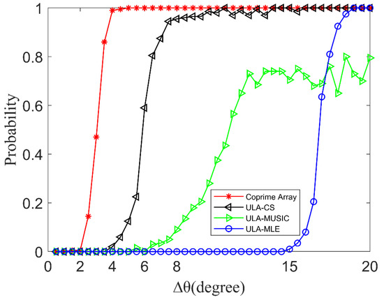
Figure 7.
The relationship between the probability that can be correctly estimated and the direct-signal DOA difference between two CCBSs.
Figure 7 shows that the three spatial spectrum estimation algorithms of the traditional ULA have poor performance. With the proposed method, when the difference between the direct-signal DOA of the two CCBSs is greater than 4°, the probability of correctly estimating the two targets after sparse reconstruction is greater than 0.99. The proposed method has better high-resolution performance, so it can have better anti-mainlobe interference capability in practical applications.
3.2.3. Performance Analysis of Direct-Signal High-Resolution DOA Estimation in Complex Environment
In the urban environment, when there are four CCBSs, the high-resolution performance of the proposed method is verified in this complex co-channel interference environment. Based on the simulation (3.2.2), two more CCBSs are added and the DOAs of the two added CCBSs are set to −30° and −66°, respectively. Further, 200 Monte Carlo simulations were performed at each DOA and the simulation result is shown in Figure 8.
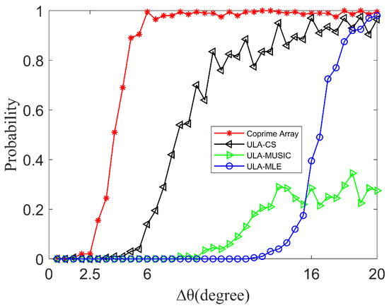
Figure 8.
The relationship between the probability that can be correctly estimated and the direct-signal DOA difference between two CCBSs when there are 4 co-frequency base stations.
Figure 8 shows that in the complex co-channel interference environment, the proposed method can correctly distinguish the two direct signals when the DOA difference between the two direct signals is greater than 6°. However, when the DOA difference between the two direct signals is greater than 16°, the probability that the compressed sensing algorithm based on ULA can correctly distinguish the two direct signals reaches 0.9 and the estimation accuracy fluctuates greatly. The other two spatial spectrum estimation algorithms based on the ULA almost fail. Compared with the traditional method, the proposed method can still obtain better high-resolution performance in the complex co-channel interference environment.
3.2.4. Performance Analysis of the Accuracy of Enumerating All CCBSs
In actual application scenarios, the number of CCBSs is not fixed and will change. The number of CCBSs is increased from one to six and the enumeration accuracy of the proposed method is verified when the number of CCBSs is different. In each case of the number of CCBSs, we performed 200 Monte Carlo experiments. Each CCBS has one co-channel direct signal and five multipaths. Each additional CCBS will increase six co-channel interferences accordingly. In each experiment, the energies of the co-channel direct signal and multipath are randomly selected between 20 and 25 dB and 0 and 5 dB, respectively, and their DOAs are randomly selected at [−90°,90°]. Therefore, the DOA difference between any two CCBSs is random. The simulation result is shown in Figure 9.
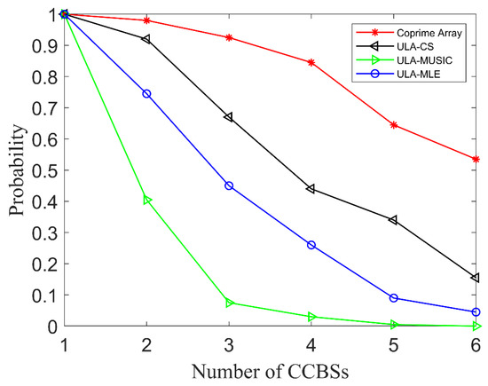
Figure 9.
All CCBSs estimate the correct probability.
In Figure 9, the horizontal axis represents the number of CCBSs and the vertical axis represents the probability that the DOA of the corresponding number of co-channel direct signal can be correctly estimated in 200 Monte Carlo experiments. As can be seen from Figure 9, when the number of CCBSs is one; that is, when there is only co-channel interference from the BS-IoO, all methods can be correctly estimated in 200 Monte Carlo experiments. This is similar to the scenario with traditional low-band radiation sources. In this case, a uniform array can be used to estimate the spatial spectrum of the CCBS. When the number of CCBSs is four, the probability that the proposed method can estimate all four co-channel direct signals in one estimation is 0.85, while the probability that the CS algorithm based on the ULA can correctly estimate is only 0.44. With the increase in the number of CCBSs, the performance of the spatial spectrum estimation algorithm based on the ULA decreases faster. When there are 6 CCBSs, a total of 36 co-channel interferences, in this complex co-channel interference environment, the probability that the proposed method can estimate all the 6 co-channel direct signals in one estimation is 0.54 and the spatial spectrum algorithms based on the ULA are almost invalid. It can be seen that the enumeration accuracy of the coprime array in the complex co-channel interference environment is better than that of the ULA with the same number of elements.
3.2.5. Performance Analysis of the Accuracy of Enumerating Some CCBSs
We hope to estimate all the co-channel direct signals in one spatial spectrum estimation, but when the number of CCBSs is large, the DOAs of all co-channel direct signals cannot be estimated in one spatial spectrum estimation. The more the number of co-channel direct signals is estimated in one simulation, the better the target detection. For this, six CCBSs were set and 200 Monte Carlo experiments were performed. In each experiment, the energies of the co-channel direct signal and multipath are randomly selected between 20 and 25 dB and 0 and 5 dB, respectively, and their DOAs are randomly selected at [−90°,90°]. The simulation result is shown in Figure 10.
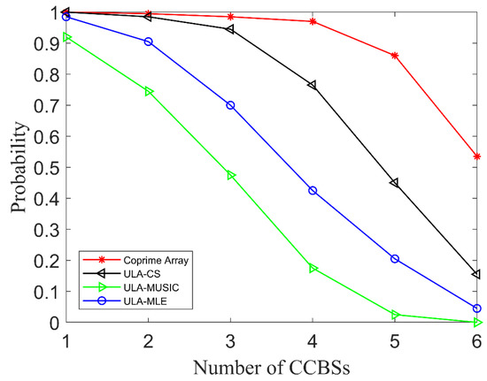
Figure 10.
The relationship between the number of CCBSs and the probability of correct estimation.
As can be seen from Figure 10, the probability that the proposed method can estimate the DOA of at least four co-channel direct signals in one estimation is 0.97 and the probability of estimating at least five co-channel direct-signal DOAs is 0.86 and the probability of estimating all six co-channel direct signals is only 0.54. The probability that the CS algorithm based on the ULA can estimate the DOA of at least five direct signals in one estimation is 0.45 and the probability of estimating all six co-channel direct signals is only 0.16. Obviously, in the complex co-channel interference environment, the enumeration accuracy of the proposed method is higher than that of the traditional method. It can be seen that in the complex co-channel interference environment, using the proposed method to estimate the spatial spectrum of the CCBS, a larger number of co-channel direct signals can be estimated each time, which will be very beneficial to the subsequent clutter elimination.
3.3. Field Experiment Results and Analysis
In this section, we analyze and verify the performance of the proposed method through experiments. The vertical polarized dipole plate-type antenna was used as the receiving antenna to receive the moving target echo and DMI from both BS-IoO and CCBS. The antenna has eight elements and the element spacing is 0.16 m. A photograph of the antenna is shown in Figure 11. The signals received undergo digital signal processing for data analysis. The 1st, 3rd, 4th and 5th elements are extracted from the ULA to form a simple coprime array with . The 6th, 7th and 8th elements of the ULA fill the right hole of the virtual array extended by the coprime array (as shown in Figure 12). The experiment location is near Xi’an Xianyang International Airport. The GSM signal was selected as the IoO for this experiment. The carrier frequency of the IoO is 957 MHz. A collection target is an aircraft that is landing or taking off. During the collection process, the normal direction of the antenna is aligned with the airport runway and the target direction is also set to about 0°. The sketch of the radar setup is shown in Figure 13, where is the bistatic angle of the radar and is the angle between the radar line of sight and the target movement path. From Figure 13, we can see that when the aircraft is taking off, the DOA of the target is gradually getting closer to the normal direction of the radar. The signal processing flow of the measured data is shown in Figure 14.
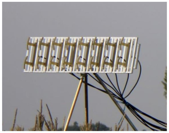
Figure 11.
Photograph of radar receiving antenna.
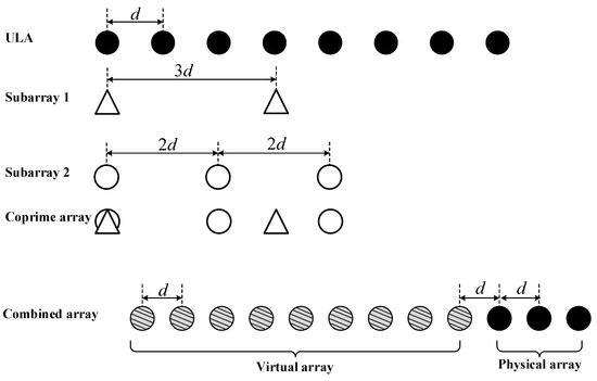
Figure 12.
Equivalent antenna schematic.
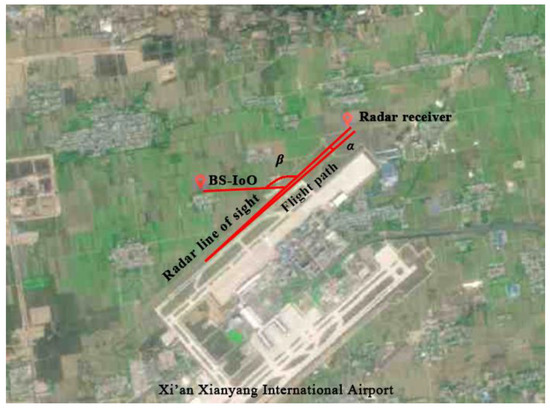
Figure 13.
Sketch of radar setup.
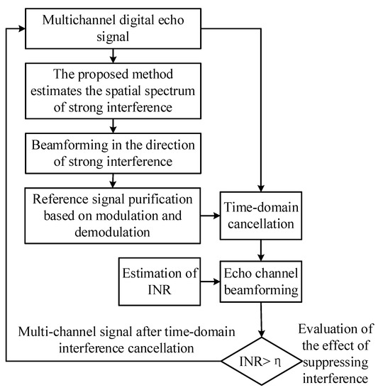
Figure 14.
The measured data processing process.
The range-Doppler cross-correlation (RDCC) is performed directly on the original echo signal and Figure 15 shows the result of RDCC.
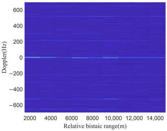
Figure 15.
The RDCC result of the original signal.
In Figure 15, the target echo cannot be seen, but we see strong interference in 0 Doppler. Because the received signal contains both the DMI from the BS-IoO and other CCBSs, at the energy level, the target echo is much smaller than the co-channel interference, causing the target echo to be submerged in it and it cannot be detected. The co-channel interference is strongest near 0 range-Doppler, which is the interference from the BS-IoO. Then, the proposed method is used to estimate the spatial spectrum of the strong co-channel interference. The spatial spectrum is shown in Figure 16.
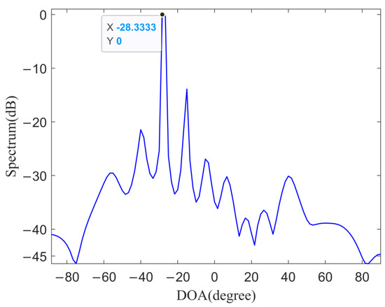
Figure 16.
The first strong co-channel interference spatial spectrum.
As can be seen from Figure 16, one peak is significantly higher than other peaks, which is the direct signal from the BS-IoO. After obtaining the DOA of the direct signal from the BS-IoO, the non-adaptive beamformer is performed to obtain the reference signal from the BS-IoO and then the ECA-B cancellation method in [35] is performed to eliminate the interference from the BS-IoO. The RDCC is performed after eliminating the interference from the BS-IoO and Figure 17 shows the result of RDCC.
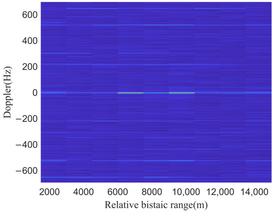
Figure 17.
RDCC after eliminating BS-IoO interference.
In Figure 17, we can see that the interference at 0 range-Doppler that appeared in Figure 15 has disappeared, indicating that the interference from the BS-IoO has been effectively suppressed, but there are still two obvious peaks in the zero-Doppler and no target is detected, because the signal received by the antenna includes a large amount of co-channel interference from other CCBSs; the energy of co-channel interference is stronger than the target echo, causing the target echo to be masked under the co-channel interference. Therefore, it is necessary to continue to eliminate strong co-channel interference. To use the ECA-B clutter cancellation algorithm to eliminate co-channel interference, it is necessary to know the DOAs of the CCBS in advance. The spatial spectrum estimation algorithms based on the ULA are limited by the spacing of the array element and the maximum cannot exceed half of the wavelength; otherwise, it will lead to angle ambiguity. When the amount of co-channel interference is large, a larger-scale array is required to improve the DOF and accuracy of the array. The coprime array breaks through the half-wavelength limit and the larger array aperture can be obtained with fewer array elements. The proposed method is used to estimate the spatial spectrum of the strong co-channel interference again and the result is shown in Figure 18.
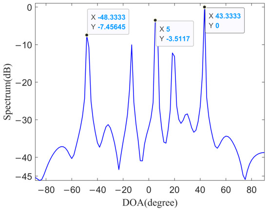
Figure 18.
The second strong co-channel interference spatial spectrum.
In Figure 18, five DOAs with strong co-channel interference are estimated by the proposed method and the interference energy in the directions of −48.3°, 5° and 43.3° is the strongest. The RDCC is performed after the three strongest interferences are eliminated from the echo channel and Figure 19 shows the result of the RDCC.
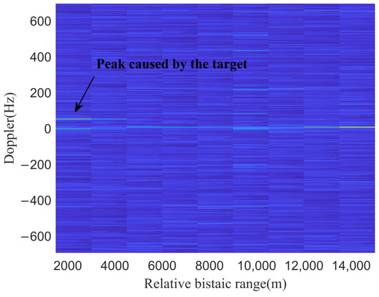
Figure 19.
RDCC after eliminating the strongest interference in Figure 18.
In Figure 19, the strongest co-channel interferences in the zero-range Doppler unit that appeared in Figure 17 are eliminated and it can be seen that a weak target echo is detected. However, there are still other strong co-channel interferences. It can be seen that the energy of the co-channel interference near 14,000 m is stronger than the target echo. Because the process of eliminating co-channel interference is to first eliminate co-channel interference with the strongest energy and then eliminate co-channel interference with the second-strongest energy step by step, weaker interference occurs in a relative bistatic range of 14,000 m, which was previously covered by the stronger interference. It is necessary to continue to perform spatial spectrum estimation on co-channel interference and obtain reference signals to eliminate these interferences. The result of spatial spectrum estimation with the proposed method is shown in Figure 20.
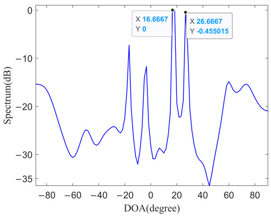
Figure 20.
The third strong co-channel interference spatial spectrum.
It can be seen from Figure 20 that the energy of the interference is strongest in the 16.6° and 26.6°. The RDCC is performed after eliminating the interference signals whose DOAs are 16.6° and 26.6° and Figure 21 shows the result of RDCC.
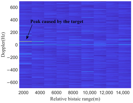
Figure 21.
RDCC after eliminating the strong interference in Figure 20.
The clear target echo can be seen in Figure 21, indicating that most of the co-channel interference has been eliminated. There are some interferences with the weaker energy, but they do not affect the target detection and do not need to be eliminated. As can be seen from Figure 22, the strong co-channel interference near 0 Doppler was eliminated. This shows that the method proposed can be used in the estimation of the co-channel interference spatial spectrum.
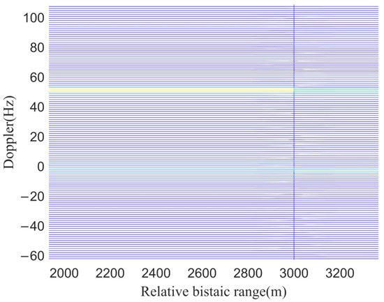
Figure 22.
Zoomed in near 0 Doppler.
In the measured data, the proposed method is used to estimate the spatial spectrum of the CCBS, which provides a basis for beamforming to obtain the direct reference signal of the CCBS. After processing multiple frames of data, the tracking result of the target Doppler trajectory is obtained, as shown in Figure 23, which verifies that the proposed method can be applied in practical scenarios.
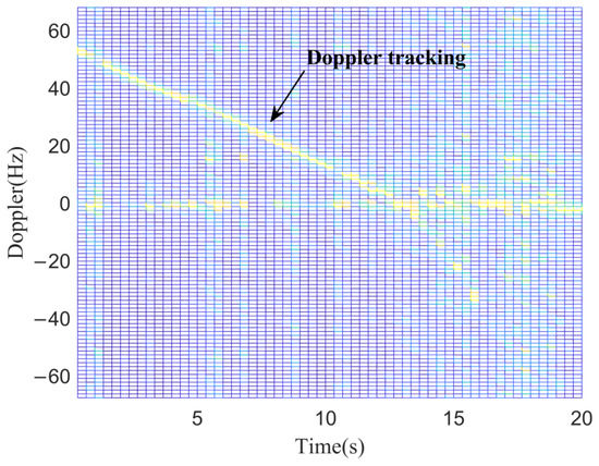
Figure 23.
Target Doppler trajectory tracking results.
4. Discussion
This study investigates the problem of obtaining the spatial spectrum of the co-channel direct signal in the complex co-channel interference environment of passive radar based on mobile communication signals. In practical application scenarios, passive radar based on mobile communication suffers from severe co-channel interference, which affects target detection. The premise of eliminating co-channel interference is to obtain the spatial spectrum of the CCBS. The method we propose is to fuse coprime array and compressed sensing to estimate the spatial spectrum of the CCBS.
The authors of [17,29,30,31] used a ULA to estimate the spatial spectrum of the direct signal of the CCBS. These methods based on ULA are applicable when there is only one CCBS (that is, BS-IoO). However, the CCBSs are densely distributed and adopt the transmission method of frequency division multiple access, which causes the mobile communication passive radar to face a large amount of co-channel interference. The amount of co-channel interference is much larger than the number of array elements and the methods in the literature have poor estimation performance or even fail in this complex co-channel interference environment. We propose to use the coprime array as the receiving antenna of the radar. The coprime array is a sparse array, the spacing between the array elements can be greater than half a wavelength and the array aperture is larger than that of the ULA when the number of array elements is the same. Signal processing is performed based on the virtual domain of the coprime array. The number of array elements in the virtual array is greater than the number of physical arrays, which effectively improves the DOF. Therefore, it can be used in scenarios where the amount of co-channel interference is greater than the number of array elements. We fuse coprime array and compressive sensing algorithm to realize super-resolution DOA estimation of co-channel interference in a complex co-channel interference environment.
In Section 3.2.1, we can see that the proposed method can effectively estimate the spatial spectrum of the co-channel direct signal in a complex co-channel interference environment. Traditional uniform arrays based on subspace classes, maximum likelihood and compressed sensing algorithms cannot be effectively estimated or may even fail. In Section 3.2.2 and Section 3.2.3, the proposed method has better high-resolution performance than traditional methods and, thus, has better anti-mainlobe interference capability in practical applications. The high-resolution performance of the proposed method can obtain a more accurate DOA of the direct signal of the CCBS and can obtain a purer reference signal, which is very beneficial for subsequent clutter elimination and target detection. In Section 3.2.4 and Section 3.2.5, we simulate the enumeration accuracy between the proposed method and the traditional method in a complex co-channel interference environment. The enumeration accuracy of the proposed method is much higher than that of the traditional method. The number of co-channel direct signals that can be estimated in one spatial spectrum estimation is larger than that of the traditional method. This will be very beneficial for subsequent clutter cancellation. The proposed method is verified by experiments. In the experiment, the proposed method is used to estimate the spatial spectrum of the co-channel direct signal. After eliminating the strong co-channel direct signal, the track of the target can be obtained after multi-frame processing.
Numerical simulations show that the proposed method has significantly better spatial spectrum estimation performance for co-channel direct signals than the traditional methods in a complex co-channel interference environment. The experimental method verifies that the proposed method can be applied in practical scenarios.
5. Conclusions
Passive radar based on mobile communication has many advantages, but it faces serious co-channel interference in practical applications, which leads to the inability to effectively detect the target, resulting in missed detection. In this paper, a CCBS direct-signal spatial spectrum estimation method fusing coprime array and compressed sensing is proposed to assist in suppressing co-channel interference. We convert the received signal of the extended coprime array to the virtual domain and the array aperture of the virtual domain array is far greater than the ULA under the same array element, which creates conditions for improving the resolution and DOF. Then, the compressive sensing algorithm is used in the virtual domain to estimate the spatial spectrum of the co-channel interference. The proposed method is compared with the MUSIC, maximum likelihood and compressed sensing algorithms based on ULA in terms of array DOF, resolution and enumeration accuracy. The simulation results show that the proposed method is superior to the traditional method in a complex co-channel interference environment. Finally, the proposed method is verified by experiments in the GSM passive radar and the results show that the proposed method can be applied to the actual mobile communication passive radar scene.
Author Contributions
Conceptualization, H.W., H.X. and K.L.; Data curation, H.W., H.X., K.L., S.O. and Y.G.; Writing—original draft, H.W. and H.X.; Writing—review and editing, K.L., S.O. and Y.G. All authors have read and agreed to the published version of the manuscript.
Funding
This work was funded by Guangxi special fund project for innovation-driven development, grant no. GuikeAA21077008, Guangxi science and technology base and talent project, grant no. AD20297038, Guangxi Key Laboratory of Wireless Wideband Communication and Signal Processing, grant no. GXKL062001018.
Data Availability Statement
The study did not report any data.
Acknowledgments
We thank all editors and reviewers for their valuable comments and suggestions for improving this manuscript.
Conflicts of Interest
The authors declare no conflict of interest.
References
- Kuschel, H.; Cristallini, D.; Olsen, K.E. Tutorial: Passive radar tutorial. IEEE Aerosp. Electron. Syst. 2019, 34, 2–19. [Google Scholar] [CrossRef]
- Liu, Y.; Yi, J.; Wan, X.; Zhang, X.; Ke, H. Time-Varying Clutter Suppression in CP-OFDM Based Passive Radar for Slowly Moving Targets Detection. IEEE Sens. J. 2020, 20, 9079–9090. [Google Scholar] [CrossRef]
- Liu, Y.; Liao, G.; Xu, J.; Yang, Z.; Yin, Y. Improving Detection Performance of Passive MIMO Radar by Exploiting the Preamble Information of Communications Signal. IEEE Syst. J. 2021, 15, 4391–4402. [Google Scholar] [CrossRef]
- Li, Z.; Huang, C.; Sun, Z.; An, H.; Wu, J.; Yang, J. BeiDou-Based Passive Multistatic Radar Maritime Moving Target Detection Technique via Space-Time Hybrid Integration Processing. IEEE Trans. Geosci. Remote Sens. 2022, 60, 5802313. [Google Scholar] [CrossRef]
- Howland, P.E.; Maksimimuk, D.; Reitsma, G. FM radio based bistatic radar. IET Radar Sonar. Navig. 2005, 152, 107–115. [Google Scholar] [CrossRef]
- Edrich, M.; Schroeder, A.; Winkler, V. Design and performance evaluation of a mature FM/DAB/DVB-T multi-illuminator passive radar system. IET Radar Sonar. Navig. 2014, 8, 114–122. [Google Scholar] [CrossRef]
- Coleman, C.; Yardley, H. Passive bistatic radar based on target illuminations by digital audio broadcasting. IET Radar Sonar. Navig. 2008, 2, 366–375. [Google Scholar] [CrossRef]
- Gómez-del-Hoyo, P.-J.; Jarabo-Amores, M.-P.; Mata-Moya, D.; del-Rey-Maestre, N.; Rosa-Zurera, M. DVB-T receiver independent of Channel allocation, with frequency offset compensation for improving resolution in low cost passive radar. IEEE Sens. J. 2020, 20, 14958–14974. [Google Scholar] [CrossRef]
- Colone, F.; Falcone, P.; Bongioanni, C.; Lombardo, P. WiFi-Based Passive Bistatic Radar: Data Processing Schemes and Experimental Results. IEEE Trans. Aerosp. Electron. Syst. 2012, 48, 1061–1079. [Google Scholar] [CrossRef]
- Tan, D.K.P.; Sun, H.; Lu, Y.; Lesturgie, M.; Chan, H.L. Passive radar using Global System for Mobile communication signal: Theory, implementation and measurements. IET Radar Sonar. Navig. 2005, 152, 116–123. [Google Scholar] [CrossRef]
- Sun, H.; Tan, D.K.P.; Lu, Y. Aircraft target measurements using A GSM-based passive radar. In Proceedings of the 2008 IEEE Radar Conference, Rome, Italy, 26–30 May 2008; pp. 1–6. [Google Scholar] [CrossRef]
- Salah, A.A.; Raja Abdullah, R.S.A.; Ismail, A.; Hashim, F.; Abdul Aziz, N.H. Experimental study of LTE signals as illuminators of opportunity for passive bistatic radar applications. IET Radar Sonar. Navig. 2014, 50, 545–547. [Google Scholar] [CrossRef]
- Geng, Z.; Xu, R.; Deng, H. LTE-based multistatic passive radar system for UAV detection. IET Radar Sonar. Navig. 2020, 14, 1088–1097. [Google Scholar] [CrossRef]
- Salah, A.A. Feasibility study of LTE signal as a new illuminators of opportunity for passive radar applications. In Proceedings of the 2013 IEEE International RF and Microwave Conference (RFM), Penang, Malaysia, 9–11 December 2013; pp. 258–262. [Google Scholar] [CrossRef]
- Samczyński, P.; Abratkiewicz, K.; Płotka, M.; Zieliński, T.P.; Wszołek, J.; Hausman, S.; Korbel, P.; Ksiȩżyk, A. 5G Network-Based Passive Radar. IEEE Trans. Geosci. Remote Sens. 2022, 60, 5108209. [Google Scholar] [CrossRef]
- Sun, H.; Tan, D.K.P.; Lu, Y.; Lesturgie, M. Applications of passive surveillance radar system using cell phone base station illuminators. IEEE Aerosp. Electron. Syst. 2010, 25, 10–18. [Google Scholar] [CrossRef]
- Wang, H.; Lyu, X.; Liao, K. Co-Channel Interference Suppression for LTE Passive Radar Based on Spatial Feature Cognition. Sensors 2022, 22, 117. [Google Scholar] [CrossRef]
- Abdullah, R. Experimental investigation on target detection and tracking in passive radar using long-term evolution signal. IET Radar Sonar. Navig. 2016, 10, 577–585. [Google Scholar] [CrossRef]
- Abdullah, R. Ground moving target detection using LTE-based passive radar. In Proceedings of the 2015 International Conference on Radar, Antenna, Microwave, Electronics and Telecommunications (ICRAMET), Bandung, Indonesia, 5–7 October 2015; pp. 70–75. [Google Scholar] [CrossRef]
- Lingadevaru, P.; Pardhasaradhi, B.; Srihari, P.; Sharma, G. Analysis of 5G New Radio Waveform as an Illuminator of Opportunity for Passive Bistatic Radar. In Proceedings of the 2021 National Conference on Communications (NCC), Kanpur, India, 27–30 July 2021; pp. 1–6. [Google Scholar] [CrossRef]
- Abdullah, R.S.A.R.; Salah, A.A.; Ismail, A.; Hashim, F.; Rashid, N.E.A.; Aziz, N.H.A. LTE-Based Passive Bistatic Radar System for Detection of Ground-Moving Targets. Etri. J. 2016, 38, 302–313. [Google Scholar] [CrossRef]
- Kiviranta, M.; Moilanen, I.; Roivainen, J. 5G Radar: Scenarios, Numerology and Simulations. In Proceedings of the 2019 International Conference on Military Communications and Information Systems (ICMCIS), Budva, Montenegro, 19 September 2019; pp. 1–6. [Google Scholar] [CrossRef]
- Griffiths, H.; Baker, C. The Signal and Interference Environment in Passive Bistatic Radar. In Proceedings of the 2007 Information, Decision and Control, Adelaide, SA, Australia, 12–14 February 2007; pp. 1–10. [Google Scholar] [CrossRef]
- Lü, M.; Yi, J.; Wan, X.; Zhan, W. Cochannel Interference in DTMB-Based Passive Radar. IEEE Trans. Aerosp. Electron. Syst. 2019, 55, 2138–2149. [Google Scholar] [CrossRef]
- Wang, H.; Lyu, X.; Zhong, L. Interference-to-noise ratio estimation in long-term evolution passive radar based on cyclic auto-correlation. Electron. Lett. 2021, 57, 375–377. [Google Scholar] [CrossRef]
- Lü, X.; Zhang, H.; Liu, Z.; Sun, Z.; Liu, P. Research on co-channel base station interference suppression method of passive radar based on LTE signal. J. Electron. Inf. Technol. 2019, 41, 2123–2130. (In Chinese) [Google Scholar] [CrossRef]
- Wielgo, M.; Krysik, P.; Klincewicz, K.; Maslikowski, L.; Rzewuski, S.; Kulpa, K. Doppler only localization in GSM-based passive radar. In Proceedings of the 2014 International Radar Conference, Lille, France, 13–17 October 2014; pp. 1–6. [Google Scholar] [CrossRef]
- Shen, J.; Yi, J.; Wan, X.; Cheng, F.; Zhang, W. DOA Estimation Considering Effect of Adaptive Clutter Rejection in Passive Radar. IEEE Trans. Geosci. Remote. Sens. 2022, 60, 5108913. [Google Scholar] [CrossRef]
- Shao, X.; Hu, T.; Xiao, Z.; Wei, Y.; Wang, H. A Co-channel Interference Suppression Algorithm for LTE-based Passive Radar. Acta Armamentarii. 2021, 42, 1670–1679. [Google Scholar] [CrossRef]
- Lu, K.; Yang, J.; Zhang, L. Extraction of Direct Signal in GSM Based Passive Bistatic Radar. Acta Armamentarii. 2014, 35, 280–284. [Google Scholar] [CrossRef]
- Wang, H.; Wang, J.; Jiang, J.; Liao, K.; Xie, N. Target Detection and DOA Estimation for Passive Bistatic Radar in the Presence of Residual Interference. Remote Sens. 2022, 14, 1044. [Google Scholar] [CrossRef]
- Zhou, C.; Gu, Y.; Fan, X.; Shi, Z.; Mao, G.; Zhang, Y.D. Direction-of-Arrival Estimation for Coprime Array via Virtual Array Interpolation. IEEE Trans. Signal Process. 2018, 66, 5956–5971. [Google Scholar] [CrossRef]
- Kim, S.-J.; Koh, K.; Lustig, M.; Boyd, S.; Gorinevsky, D. An interior-point method for large-scale l1-regularized LSs. IEEE J. Sel. Top. Signal Process. 2007, 1, 606–617. [Google Scholar] [CrossRef]
- Elgendy, O.A.; Ismail, M.H.; Elsayed, K. On the relay placement problem in a multi-cell LTE-Advanced system with co-channel interference. In Proceedings of the 2012 IEEE 8th International Conference on Wireless and Mobile Computing, Networking and Communications (WiMob), Barcelona, Spain, 8–10 October 2012; pp. 300–307. [Google Scholar] [CrossRef]
- Colone, F.; O’Hagan, D.W.; Lombardo, P.; Baker, C.J. A Multistage Processing Algorithm for Disturbance Removal and Target Detection in Passive Bistatic Radar. IEEE Trans. Aerosp. Electron. Syst. 2009, 45, 698–772. [Google Scholar] [CrossRef]


Publisher’s Note: MDPI stays neutral with regard to jurisdictional claims in published maps and institutional affiliations. |
© 2022 by the authors. Licensee MDPI, Basel, Switzerland. This article is an open access article distributed under the terms and conditions of the Creative Commons Attribution (CC BY) license (https://creativecommons.org/licenses/by/4.0/).