Abstract
The problem of multispectral and hyperspectral image fusion (MHF) is to reconstruct images by fusing the spatial information of multispectral images and the spectral information of hyperspectral images. Focusing on the problem that the hyperspectral canonical polyadic decomposition model and the Tucker model cannot introduce the physical interpretation of the latent factors into the framework, it is difficult to use the known properties and abundance of endmembers to generate high-quality fusion images. This paper proposes a new fusion algorithm. In this paper, a coupled non-negative block-term tensor model is used to estimate the ideal high spatial resolution hyperspectral images, its sparsity is characterized by adding 1-norm, and total variation (TV) is introduced to describe piecewise smoothness. Secondly, the different operators in two directions are defined and introduced to characterize their piecewise smoothness. Finally, the proximal alternating optimization (PAO) algorithm and the alternating multiplier method (ADMM) are used to iteratively solve the model. Experiments on two standard datasets and two local datasets show that the performance of this method is better than the state-of-the-art methods.
1. Introduction
Hyperspectral sensors are capable of imaging target regions in multiple parts of the electro-magnetic spectrum; for example, ultraviolet, visible, near-infrared, and infrared, in dozens or even several hundred consecutive, relatively narrow bands simultaneously, acquiring images with high spectral resolution but low spatial resolution [1]. In other words, the images are acquired by perceiving the sunlight reflected from the object or scene, and the spatial resolution is inevitably reduced due to the limited solar irradiance [2]. Multispectral sensors, in contrast, acquire images with higher spatial resolution, but with insufficient spectral resolution. Thus, hyperspectral imagers (HSIs) are three-dimensional data cubes with two spatial dimensions and one spectral dimension, where the spectral dimension provides the power to identify materials in the scene. It makes HSI abundant in spectral information, which can be effectively used to improve the performance of computer vision and remote sensing. Additionally, multispectral imagers (MSIs) contain abundant spatial information. However, spectral and spatial information is crucial in hyperspectral imaging applications (e.g., image recognition, agricultural monitoring, etc.), and so multispectral and hyperspectral image fusion (MHF) techniques are catching the interest of researchers. MHF can fuse HSI and MSI to obtain high spatial resolution hyperspectral images (HRHSs). Among them, HSI has abundant spectral information and poor spatial resolution, while MSI is mainly characterized by less spectral information but high spatial resolution. Due to physical constraints, HRHS cannot be acquired by a single sensor at present.
Early spatial–spectral fusion research was extended via panchromatic sharpening, which produces high-resolution multispectral images (HR-MSI) mainly by fusing panchromatic images (PANs) with low spatial resolution MSIs. Existing panchromatic sharpening methods mainly add details from panchromatic images to MSIs to generate HR-MSIs. Meng et al. in [3] divided the panchromatic sharpening methods into component replacement (CS) [4,5] and multi-resolution analysis (MRA) [6,7,8]. They are mainly based on wavelet techniques [9,10], intensity hue saturation (IHS) methods [11], principal component analysis (PCA) [12], Laplace’s pyramid [13], or attempts at the generalized sharpening algorithms of CS and MRA for MHF problems [14]. However, in the course of extensive practice, it was found that these methods do not improve the spatial resolution of each hyperspectral band very well [15]. In recent years, with the update of algorithms, more and more researchers are interested in the MHF problems, which makes the solution for the MHF problem continuously in development. To a great extent, it promotes the development of diversity in MHF techniques. Low-rank matrix decomposition-based methods [16,17,18,19,20,21,22] and tensor-based methods [23,24,25,26,27,28,29,30] are widely popular.
In 2011, Yokoya et al. proposed a coupled non-negative matrix decomposition (CNMF) [16] method for MSI and HSI fusion problems in which the alternate spectral unmixing of the non-negative matrix decomposition (NMF) was used to estimate the abundance matrix and the endmembers matrix, but the fusion results were not satisfactory because the cost function of NMF was nonconvex. Simoes and Wei et al. proposed Hysure [19] and FUSE [20] successively by considering the target image as a low-rank matrix, but the results were also unsatisfactory. In 2018, Kanatsoulis [31] et al., based on the fact that both HSI and MSI are composed of a “cube” of “space × space × spectrum”, a new idea based on the coupled tensor decomposition (CTD) framework is proposed to solve the MHF problem. Here, the spectral image is formulated as a third-order tensor, the HSI-MSI fusion problem is solved using the coupled canonical polyadic decomposition (CPD) model, and the uniqueness of CPD is exploited. The recoverability of HRHS under mild conditions is demonstrated. In the literature [23], a similar idea was adopted to solve the MHF problem using Tucker decomposition. In 2020, Xu [25] et al. proposed a new hyperspectral super-resolution method based on unidirectional total variational (TV). The method uses the Tucker decomposition to decompose the target HRHS using a sparse core tensor, which is decomposed using a three-mode dictionary matrix, and then applies the norm to the core tensor to express the sparsity of the objective HRHS, and applies the unidirectional TV canon to the three-mode dictionary to represent the segmental stability of the objective HRHS. Although CPD and Tucker show good recoverability for MHF problems and both frameworks exhibit excellent performance, the physical interpretation of the underlying factors is unintroduced into the framework. In the presence of noise or modeling errors, the endmembers and abundance information cannot be used to produce better fusion results. Therefore, the canonical polyadic (CP) and Tucker methods are by no means necessarily better than the low-ranked matrix-based estimation methods, which do without recoverable support.
In contrast, the linear mixed model (LMM), which utilizes matrixed HSI and MSI low-rank structures, excels in this regard with a strong physical interpretation of the underlying factors (i.e., endmembers and abundance). In addition, many structural constraints and regularizations can be applied to improve algorithm capabilities. This information becomes more important when the data is noisy. However, the key to solving MHF using LMM is whether recovered HRHS can be identified. Some work in the literature [30] shows that under relatively restricted conditions, coupled matrix decomposition models are identifiable to recover HRHS, such as: the abundance matrix of MSI has sparsity. Based on this, Zhang [32] et al. in 2019 proposed to solve the hyperspectral super-resolution (HSR) problem using the block-term tensor decomposition (BTD) [33,34,35] model. When modeling the spectral image as a BTD model, the potential factors have explicit physical meaning, while the spectral image key components are also incorporated into the model, such as the endmembers and non-negative abundance maps, and spectrally and spatially smooth a priori information. The algorithm does not consider more types of regularization and constraints, and does not test the algorithm in multiple scenarios, which has limitations. In 2021, Ding [36] et al. formulated the HSR problem as a coupled LL1 tensor decomposition model, proved BTD recoverability, ensured that theoretical guarantees were not lost when using the LL1 model, and added regularization terms to improve the algorithm performance. However, the algorithm does not take the individual abundance matrices into account and the implementation scenario is limited to satellite images. Therefore, to take full advantage of the physical interpretation of the potential factors in the MHF problem, the algorithm performance is improved. In this paper, we propose a coupled non-negative BTD model to estimate HRHS and inscribe its sparsity by adding parametrization while introducing TV to inscribe segmental smoothness. The difference operators in the horizontal and vertical directions are added to the algorithm in this paper; the proposed algorithm in this paper is called 2D-CNBTD. The contributions of the proposed method are as follows.
- (1)
- In the process of recovering high spatial resolution hyperspectral images (HRHS), considering the sparsity of the endmember matrix and the abundance matrix, the norm representing sparsity is used to improve the performance of the fusion algorithm.
- (2)
- Because there is always noise and a non-smooth phenomenon in the acquired image, in order to avoid this phenomenon, two different operators are defined, into which are described their segmental smoothing.
- (3)
- During the experiment, not only are two different standard datasets, but also two local datasets about Ningxia are used to make the algorithm adaptability more extensive and its performance more convincing.
2. Background
Since HSI can be considered as a third-order tensor (three-dimensional array); here, it can be understood as a generalization of vectors and matrices. In existing research on fusion algorithms, low-ranked tensor-based methods are commonly used, while tensor-based methods are broadly classified into CP and Tucker decomposition models.
The CPD model [37] is arguably the most popular tensor rank decomposition model, and is also called the parallel factor analysis model (PARAFAC), which decomposes a tensor into a sum of multiple single-rank tensors; the process is shown in Figure 1. Under the CP model, a third-order tensor of rank R is transformed into a sum of tensors of rank one, which could be built as (see Appendix A for details of symbolic remarks in the text):
where , , are the factor matrices of the third-order tensor , respectively.
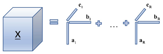
Figure 1.
Canonical polyadic decomposition process.
In addition, the Tucker model [38], which has been extensively applied in the imaging field, could be considered as a high-order version of PCA [12], which decomposes the tensor into a core tensor and three factor matrices; the process is shown in Figure 2. It is capable of being expressed as:
where , , is a set of factor matrices and is a third-order core tensor.
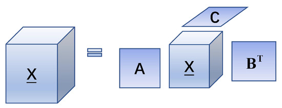
Figure 2.
Tucker decomposition process.
By combining the advantages of the CP decomposition and the Tucker decomposition, the BTD [39] of rank- can be formulated generally in terms of:
where , , , . It is observed that BTD aims to approximate through R component tensors; each tensor is represented by the Tucker decomposition of rank-. Assume that the rank of every component tensor of BTD is one; it can be considered as a CPD. Alternatively, when , the above model can be viewed as the Tucker decomposition of rank-. Therefore, the BTD can be regarded as a combo of CPD and Tucker decomposition, and the decomposition model is shown in Figure 3.
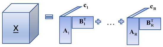
Figure 3.
Block-term tensor decomposition process.
In this paper, we select a special model of the BTD, the BTD of rank-, which can be formulated as:
where , for and . We further stated , ; where the partition matrices and have full column rank and do not have any colinear columns, with . The usual full column rank requirement for A and B is . Under a mild condition, the BTD of rank- also has the nice property where and are identifiable until the alignment and scaling ambiguities arise, with the following lemma ([34] Theorem 4.7):
Proof of Theorem 1.
Let represent a BTD of in rank- terms. Assume that are drawn from certain joint absolutely continuous distributions. If and , then are essentially and almost definitely unique. □
3. MHF Method Based on the Coupled LL1 Model
3.1. Linear Mixed Model (LMM) and Multilinear Rank Model (LL1)
The classical LMM is first introduced to facilitate an understanding of how the matrix decomposition-based approach utilizes physical interpretation. Set HRHS as the objective image. According to the LMM, the three-mode matrix is denoted [40] as follows:
where contains the matrix of spectral properties of the endmembers, and ; is the abundance matrix. The abundance map of an endmembers r can be expressed as , where the operation is to reshape the vector of size into a matrix of size . Assumptions: each abundance map is obtained via an approximation of a low-rank matrix of rank-. i.e.,:
where , . Since the distribution of pixels in the space is not random, the assumption about the low rank of the approximate is justified. Thus, assuming that the abundance map is low-rank and reshapes Equation (8) in terms of a tensor, then the tensor is expressed as:
Setting rank = , Equation (10) could be rewritten as:
The tensor model in Equation (11) is the LL1 model that this paper needs. The main task in the reconstruction of HRHS is to recover HRHS from MSI and HSI obtained in the same environment. Therefore, our purpose was how to evaluate the potential factors A, B, and C from MSI and HSI to reconstruct the HRHS by Equation (11).
3.2. Coupling LL1 Tensor Decomposition Modeling
The HSI and MSI can be denoted by the constants and of the third-order tensor. Respectively, where , , , and denote the spatial dimensions, and indicates the spectral band amounts. Therefore, all the spectral images can be expressed in the form of “space × space × spectrum”. In general, MSI has finer spatial information than HSI due to the sensor characteristics, i.e., , and . We assume that both MSI and HSI are obtained via HRHS downsampling/degradation, where HRHS has the space resolution of MSI and the spectral resolution of HSI .
The LL1 model on HRHS is derived by assuming that the abundance map is a low-rank matrix.
where , , , . In turn, HSI can be interpreted as a space-blurred and down-sampled version of HRHS.
Therefore, it is modeled by multiplying the two fuzzy and compressed matrices via the row and column dimensions of each -component tensor, as follows [36].
where and denote the upper spatial fuzzy and downsampling matrices along the two spatial dimensions, respectively. The process is shown in Figure 4.
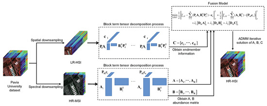
Figure 4.
The flow chart of the algorithm in this paper.
If conforms to the LL1 model, as well as the space degeneracy pattern holds in Equation (13), the mathematical model of is shown below:
MSI can be expressed as the spectral band aggregation form of HRHS, and the mathematical model is shown below (see Figure 4 for the procedure):
where is the band aggregate matrix associated with sensor specification, and then Equation (15) is compactly expressed as follows:
Under this degenerate model, the main primary goal of recovering is to identify (endmembers) from and the potential factor (abundance map) from . Once and are identified, they can be reconstructed by using .
In particular, it should be noted that the BTD model is more attractive than the CP and Tucker models in solving the MHF problem. This is because and represent the abundance and endmembers, respectively, with physical significance such as non-negativity and spatial smoothness, which help to regulate the MHF criteria with a priori knowledge. The previous one represents the abundance information of the endmembers r, and the latter represents the rth endmember. Based on the description of problem (10) and the downsampling along the three dimensions, in the absence of noise, the MHF problem based on the coupled LL1 model is described as follows.
3.3. Modeling
In the former two sections, we describe in detail the relationship between the LMM model and the LL1 model, together with a re-simulation of the MHF problem using the LL1 model. Through the above analysis, it can easily establish the fact that the LMM model and the LL1 model are consistent. Therefore, the potential factors of the LL1 model are physically interpretable, which allows us to fully exploit the prior information of endmembers and the abundance information of to enhance the fusion effect in the presence of a large amount of noise. However, this does not mean that the fusion effect of the MHF problem can be optimized, and the parametrization and TV, which are effective means to describe sparsity and segmental smoothness. Introduce them into the model and add some rule terms and constraints in A, B, and C, to further improve the fusion effect. The following modified form is proposed for model (17).
where is the regularization parameter and is the limited differencing operator in the vertical and horizontal directions.
For the proposed new modification scheme, there are the following considerations: Firstly, the proposed model (17) is based on the noise-free case, in order to recover HRHS accurately, and when there is a lot of noise in MSI and HSI, the scheme will no longer be applicable, so it needs to impose constraints on it by adding some penalty terms to prevent the model from overfitting and limiting the complexity. Secondly, according to the properties of the LL1 model, where A, B, and C have good physical properties, it is easy to exploit the various prior information present in them, e.g., A, B, and C are non-negative [20,41]; MSI and HSI acquired in the same scenario, and are coupled. Finally, considering sparsity and segmental smoothing, this paper defines two difference operators, and , for the properties of A, B, and C (see Equations (19) and (20)), while adding regularization and imposing non-negative constraints on them, to effectively maintain edge information and preserve the smoothness of the local spectra.
The flow chart of the proposed algorithm in this paper is shown in Figure 4. Firstly, the low-resolution hyperspectral images (LR-HSI) and the high-resolution multispectral images (HR-MSI) are obtained by downsampling the Pavia University dataset. Secondly, the LR-HSI and HR-MSI are decomposed using BTD to obtain the endmember matrix C of LR-HSI and the abundance matrix A, B of HR-MSI, which are brought into the model (18). Finally, the alternating directional multiplier method (ADMM) is used to iteratively solve A, B, C, which is brought into Equation (12) to obtain the target image HRHS.
Next, this paper gives the efficient solution algorithm for the model (18). Since the problem is a nonconvex optimization problem, where A, B, and C are coupled variables, the optimization issue was convex for every variable, while keeping the other variables constant. Therefore, each variable is solved iteratively with the help of the proximal alternating optimization (PAO) [42,43] method.
Model (18) is solved by using PAO with the following procedure.
where is an implicit representation of model (18). and represent the result of the preceding iteration and a non-negative value, separately.
In the following, a detailed formulation of the A optimization problem in the model (18), and the B and C optimization problems are shown in Appendix B.
Optimization Problem on A
Fixing B, C, the optimization problem on A in the above equation is shown as follows:
Via the mode-1 expansion, and through the introduction of the splitting variable , problem (22) can be formulated anew as:
where and is obtained by matrixing Equation (5) to obtain the augmented Lagrangian function for problem (23).
where is the Lagrangian multiplier and is the positive penalized parameter.
For problem (24), the ADMM iterative equation is shown below:
In the following, the solution procedure of problem (25) is given.
- Subproblem of A: for problem (24), the minimization objective function is as follows:Problem (26) is a quadratic optimization problem whose solution is unique. Compute Sylvester’s equation to solve A by calculating the following, i.e.:In this paper, this problem is effectively solved by using CG [44].
- Subproblem of : For problem (24), the minimization objective function is as follows:The solution of its is well known as a soft threshold, i.e.:where .
- Subproblem of : For problem (24), the updated Lagrange multiplier is given by:
The pseudo-code of the optimization algorithm on A is shown in Algorithm 1.
| Algorithm 1 Solving A-Subproblem (22) via ADMM. |
| Input, , , , , , , , . |
| Output Dictionary matrix A |
| While unconverged do |
| Updating the matrix A by solving problem (24) with the CG method; |
| Updating the variable by ); |
| Updating the Lagrangian multiplier L1 by L1 − (DHA − U1); |
| end While; |
4. Experiments and Analysis
4.1. Datasets
In this paper, two standard datasets and two local datasets are selected for experiments to verify the effectiveness of the proposed MHF fusion algorithm via numerical results.
4.1.1. Standard Datasets
The Pavia University dataset was obtained using the Italian Reflection Optical System Imaging Spectrometer (ROSIS) light sensor in the Pavia University downtown area. The ROSIS continuously images 115 bands in the wavelength range from 0.43 to 0.86 m, with a spatial resolution of 1.3 m and an image size of 610 × 340 × 115. After eliminating the water vapor bands, the band number decreased to 102. In view of the experimental requirements, a sub-image of size 256 × 256 × 102 is selected in the upper left part of the image as the reference image for testing.
The Indian Pine dataset was collected by the AVIRIS sensor in Indiana, with a spatial resolution of 20 m. The dataset has a large format of 144 × 144, with 224 bands. Bands 104–108, 150–163, and 220 are excluded because they cannot be reflected by water, leaving 200 bands as the object of study. For downsampling reasons, a subimage of size 144 × 144 × 200 in the upper left corner was selected as the reference image for the experiment.
4.1.2. Local Datasets
Referred to are the GF-1 and GF-5 Sand Lake datasets of Ningxia, China. In particular, the GF-1 Sand Lake dataset of Ningxia was taken by the GF-1 satellite carrying the WFV4 multispectral camera over the Sand Lake region of Ningxia on 31 July 2019, Beijing time, with each view image covering an area of about 1056.25 square kilometers, and the entire Sand Lake area accounting for about eight percent of the image. The multispectral camera continuously imaged three bands in the wavelength range of 0.45–0.89 m to obtain multispectral images, and the resulting images have a spatial resolution of 16 m and an image size of 12,000 × 13,400 × 3. The image of the Sand Lake area was selected as the MSI, which has a size of . The GF-5 Sand Lake dataset of Ningxia was taken by the AHSI sensor-equipped GF-5 satellite over the Sand Lake region of Ningxia on 27 July 2019, Beijing time, with each view image covering an area of about 3600 square kilometers, and the entire Sand Lake region covering about three percent of the image. The sensor continuously imaged 330 bands in the wavelength range of 0.4–2.5 m to obtain hyperspectral images, and the resulting images have a spatial resolution of 30 m and an image size of , with the number of bands reduced to 143 after excluding some noisy high and water vapor absorption bands. An HSI image of size was obtained by intercepting the GF-5 image at the place where the MSI image was acquired from the GF-1.
The UAV acquisition of Qingtongxia rice field dataset is a scene acquired by DJI UAV with the hyperspectral sensor Pika-L and the multispectral sensor Micasense Altum during an experimental rice field flight campaign in Qujing village, Qingtongxia, Ningxia, China, on 15 July 2021. The experimental area consisted of 19,992.71 m of paddy fields and 2134 m of houses, and the houses and courtyards accounted for 10 percent of the image in the whole image obtained. During the dataset acquisition, the UAV flew at a speed of 3 m/s, an altitude of 100 m, and a pitch angle of −90. Among them, the Pika-L hyperspectral sensor continuously imaged 150 bands in the wavelength range of 0.4–1.0 m to obtain hyperspectral images, and the spatial resolution of the generated images was 10 cm; the image size was . After removing some noisy bands, the number of bands reduced to 60, from which a sub-image of containing information on houses, rice fields, courtyards, etc., was truncated as the HSI. The Micasense Altum multispectral sensor continuously imaged three bands in the wavelength range of 0.475–0.717 m to obtain a multispectral image with a spatial resolution of 5.2 cm and an image size of 16,103 × 9677. The image size is 16,103 × 9677 × 3. A sub-image of is intercepted at the same location as the MSI. The area of the intercepted image is about one-tenth of the whole image.
4.2. Compared Algorithms
Six algorithms, CNMF [16], Hysure [19], FUSE [20], SCOTT [23], STEREO [31], and BTD [32], were selected for comparison tests in this paper. In particular, SCOTT and STEREO are based on the Tucker and CPD models for solving MHF problems, respectively. All experiments were run on a PC with an Intel(R) Xeon(R) Gold 6154 CPU @3.00 GHz and 256 GB RAM. A Windows 10 × 64 operating system was used, on which the programming software was MATLAB R2017b. The result of all the experiments is the average of 10 independent experiments.
4.3. Test Indicators
In order to better evaluate the superiority of the algorithm, and to determine the quality of the fused images, numerical results analysis is an important measure, in addition to the direct observation of the fusion results. This paper uses test metrics that are widely used in the literature [2,15]. Its detailed definition is shown below.
Peak Signal To Noise Ratio (PSNR), which evaluates the level of image distortion or noise. The general situation of PSNR is between 30 dB and 50 dB. In the ideal case, it is expected to be as high as possible, with ∞ representing the optimal value. It should be especially noted that when the PSNR is more than 30 dB, it is difficult for the human eyes to see the difference between the fused image and the reference image. The definitions are as follows.
Structural Similarity (SSIM), which is used to calculate the structural similarity between the HRHS and the reference image in the spatial domain [45]. SSIM ranges between −1 to 1. When the two images are identical, the SSIM value is equal to 1. The definitions are as follows.
Correlation Coefficient (CC), which describes the degrees of spectral likeness with respect to the objective image, as well as the fusion image. CC is based on a scale of −1 to 1. The closer the CC is to 1, the higher their positive correlation. The definitions are as follows.
Universal Image Quality Index (UIQI) [46], which is specifically used to detect the average correlation between the reference image and the fused image. If the fused image is closer to the reference image, the UIQI value is closer to the value 1, which means the better the reconstruction effect. The definitions are as follows.
Root Mean Squared Error (RMSE), which is an important index describing the root mean squared error between each band of the reference image and the fused image. If the fused image is closer to the reference image, the closer the RMSE value is to the value 0. The definitions are as follows.
Erreur Relative Globale Adimensionnelle de Synthese (ERGAS) [47] is an important measure of the global quality and spectral variability of the reconstructed image. If ERGAS is closer to the value of 0, it means the better the reconstruction effect. The definitions are as follows.
Spectral Angle Mapper (SAM) [48] is a metric used to measure the magnitude of the angle between the pixel spectra of the source image and the fused image. If the SAM value is closer to the value of 0, it means that the two images match more and the similarity is higher. The definitions are as follows.
where and the i-th band of the initial and fused images, and are the average pixel values of the initial and fusion images, respectively. , as well as are the mean values of and , respectively. , , and are expressed as standard deviation, variance, and covariance, respectively. is a constant. Here, the larger the value of PSNR, the closer the SSIM, CC, and UIQI values are to 1, and the closer the RMSE, ERGAS, and SAM values are to 0, indicating a better fusion effect.
4.4. Degradation Model
For the standard dataset, a publicly available HSI dataset was used as the reference image following the approach in the literature [20,30,49]. The simulated HSI and MSI images used in the experiments were produced according to the Wald protocol. The degradation model of the reference image to HSI is as follows: the reference image is first blurred using a 9 × 9 Gaussian kernel, and then it is downsampled every four pixels along the spatial dimension. The degradation process of the reference image to the MSI is set according to the literature [31]. In addition, zero-mean Gaussian white noise is added to the MSI and HSI.
4.5. Parameter Discussion
There are many factors that affect the fusion effect of the algorithm, and parameters are one of the important influencing factors. In this paper, it needs to consider the effect of the regularization parameter , the penalty parameter , the non-negative number , and different signal-to-noise ratios (SNRs) on the algorithm, and how to choose the appropriate R and L to make the algorithm fusion effect reach the best result.
4.5.1. , , and Parameter Selection
After conducting ablation experiments for the regularization parameter and the penalty parameter , respectively, it is found that , , and take approximately equal values, and , , and take approximately equal values. Therefore, the three parameters of , , and are set as follows: , . With regard to the choice of parameter values, the optimal value of a parameter is found by fixing two parameters and changing one parameter. Here, we select the Pavia University dataset for experiments to analyze the effect of parameter value changes on the PSNR and to select the appropriate parameter values. The regularization parameter is solved with a fixed penalty parameter and a non-negative number . While the regularization parameter grows at a rate of 10 times from 0.1, the change in the PSNR line chart is observed and the optimal value is selected. Similarly, the values of the penalty parameter and the non-negative number are obtained. As shown in Figure 5, the PSNR gradually stabilizes as the three parameters keep changing, and the parameter value corresponding to the time when the PSNR is maximum is selected. Therefore, the values of the three parameters are set as follows: , , .
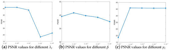
Figure 5.
(a–c) PSNR values for the Pavia University dataset for the variation of parameters , , and .
4.5.2. R and L Discussion
In the algorithm proposed in this paper, the matrix rank R and L of will be different for different datasets, and the variation of R and L will have a great impact on the performance of the fusion algorithm. Therefore, in order to make the algorithm achieve the best fusion effect on the Pavia University dataset and the Indian Pine dataset, the values of R and L need to be determined experimentally.
The PSNR values for different R and L in the Pavia University dataset are given in Figure 6. In the experiments, since the R and L values are uncertain, only rough estimates of R and L can be made initially, and then the experiments are repeated by choosing different values of R and L and finding the best values around the estimates. Thus, is set for an uncertain L value, resulting in Figure 6a. Similarly, is set for an uncertain value of R, resulting in Figure 6b, where the PSNR increases gradually when R is taken at . At the value of , the PSNR remains flat. The PSNR increases gradually when L is taken at . The PSNR remains smooth when is taken. Therefore, this is set to: , .
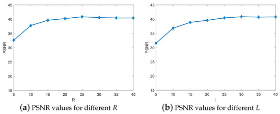
Figure 6.
(a,b) PSNR values for different R and L in the Pavia University dataset.
The PSNR values for different R and L in the Indian Pine dataset are given in Figure 7. In the case of uncertainty in the value of L, set , which yields Figure 7a. Similarly, set for an uncertain value of R, resulting in Figure 7b, where the PSNR increases gradually when R is taken at . At , the PSNR remains stable. The PSNR increases gradually when L is taken at . The PSNR remains smooth at . Therefore, R and L are set as follows: , .
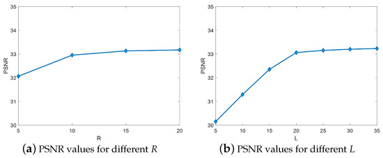
Figure 7.
(a,b) PSNR values for different R and L in the Indian Pine dataset.
4.5.3. SNRs Discussion
The Signal-to-Noise Ratios (SNRs) also affect the fusion effect of algorithms. In order to avoid the comparison of “optimal” and “non-optimal” effects between algorithms, it is necessary to select a suitable SNR value to ensure that all algorithms have achieved the best effect at that SNR value, and then discuss the superiority of the algorithms. The Pavia University dataset is selected for SNRs discussion in this paper. Before conducting the experiments, all parameters in the algorithm experiments have been tuned to be optimal. The SNRs were selected in the range of 15 dB–40 dB. Figure 8 plots the variation of evaluation metrics for all algorithms at different SNRs. From the figure, it can be seen that all algorithm curves level off after = 30 dB. Therefore, Pavia University dataset SNRs are set to = 30 dB.
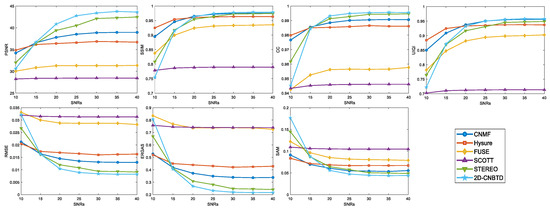
Figure 8.
Plot of the change in evaluation metrics for all algorithms in the Pavia University dataset at different SNRs.
4.6. Validity of the Regularization Terms
In the model (18) of the algorithm proposed in this paper, the smoothness and sparsity of the fusion algorithm are described using three regularization terms , , and . In order to verify whether the algorithm in this paper is improved, experiments were conducted using the BTD algorithm and the proposed algorithm in this paper on the Pavia University dataset, the Indian Pine dataset, the GF-1 and GF-5 Sand Lake in Ningxia of China dataset, and the UAV Acquisition of the Qingtongxia Rice Field dataset, respectively. The numerical information derived from the experiments is shown in Table 1. In which, the time unit is seconds, and the optimal value is noted as 0 s; bold in the table indicates better values; and PSNR, SSIM, and other test metrics are described in detail in Section 4.3. From Table 1, it can be seen that the algorithm in this paper has substantially improved SSIM and UIQI, which describe the spatial feature metrics, compared to before the improvement. The indicators CC, RMSE, and SAM about the spectral features are also significantly improved, but the time is slightly increased by 3 s–9 s. It shows that although the improved algorithm has a slightly longer running time, it can better retain the spatial and spectral information of the image during the image fusion process, which makes the fused image clearer.

Table 1.
Comparison of BTD and 2D-CNBTD values.
4.7. Experimental Results for Standard Datasets
The fusion results of the seven tested methods on the Pavia University and Indian pine datasets are shown in this section.
4.7.1. Experimental Results of Pavia University Dataset
To demonstrate the spatial detail information, reconstruction effect, and fusion results, three bands (R: 61, G: 25, B: 13) are selected to synthesize pseudo-color images in this paper. Set = 30 dB. The fusion performances of all methods on the Pavia University dataset are plotted in Figure 9. Figure 9h shows the reference image, and the scene in the red box is shown in the upper left corner of the figure.
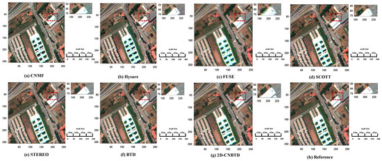
Figure 9.
Graph of reconstructed HRHS results for Pavia University dataset.
When the difference between HRHS and the reference images is small, it is difficult to find out the difference using the human eye. Therefore, some evaluation metrics are used to analyze the algorithm’s performance. These evaluations of the compared algorithms are shown in Table 2, and the better results are indicated in bold in the experiments. In terms of spatial features, both the algorithm in this paper and CNMF are closer to 1 in terms of the SSIM and UIQI values, but in comparison, the algorithm in this paper performs better in SSIM, which indicates that it is more similar to the reference image in terms of contrast, brightness, and spatial structure. The two algorithms have similar values in UIQI, which means that the fused image has the least loss of correlation information and is highly similar to the reference image. As far as the spectral features, the CC of this paper’s algorithm is closer to 1, and the RMSE, ERGAS, and SAM are closer to 0, indicating that the spectral distortion of the fused image of this paper’s algorithm is the smallest, which is consistent with the spectral features of the reference image. From the value of PSNR, the algorithm in this paper has the highest PSNR, which indicates that the algorithm in this paper can effectively reject the noise. The algorithms have moderate running times.
Table 2.
Performance for Pavia university.
4.7.2. Experimental Results of the Indian Pine Dataset
To demonstrate the spatial detail information, reconstruction effect, and fusion results, three bands (R: 61, G: 25, B: 13) are selected to synthesize pseudo-color images in this paper. Set dB. The fusion performances of all methods on the Indian Pine dataset are plotted in Figure 10. Figure 10h shows the reference image, and the scene in the red box is shown in the upper left corner of the figure.
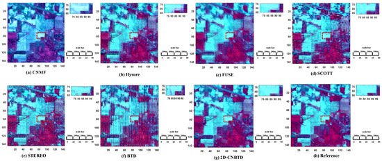
Figure 10.
Graph of reconstructed HRHS results for Indian Pine dataset.
Here, the performance of the algorithm is analyzed using a selection of evaluation metrics. The evaluations of the compared algorithms are shown in Table 3, and the better experimental results are indicated in bold. In terms of spatial characteristics, both the algorithm in this paper and CNMF are closer to 1 in terms of the SSIM and UIQI values, but in comparison, the paper algorithm performs better in UIQI, which indicates that the fused image has the least loss of relevant information and is highly similar to the reference image. The similar values of both algorithms on SSIM indicate that they are more similar to the reference image in terms of contrast, brightness, and spatial structure. In terms of the spectral features, the CC of the algorithm in this paper is closer to 1, and the RMSE, ERGAS, and SAM are closer to 0, suggesting that its fused image has the least spectral distortion and is consistent with the spectral features of the reference image. From the value of PSNR, the algorithm in this paper has the highest PSNR, which indicates that the algorithm in this paper can effectively eliminate noise. The running time of the algorithm is reasonable.
Table 3.
Performance for Indian Pines.
4.8. Experimental Results for Local Datasets
4.8.1. GF-1 and GF-5 Sand Lake in Ningxia of China
For the GF-1 and GF-5 Sand lake datasets in Ningxia, both datasets have been aligned and corrected usin ENVI 5.3. Due to the specificity of the satellite, the two datasets are treated as if they were taken at the same time. Regarding the three parameters , , and , the previous settings are followed. R and L are set via an ablation experiment: , . Here, the MSI and HSI image size ratio is 1:1, and the MSI and HSI of the same scene are directly fused without the spectral degradation and spatial degradation processes. To demonstrate the spatial detail information, reconstruction effect, and fusion results, three bands (R: 59, G: 38, B: 20) are selected to synthesize pseudo-color images in this paper. The fusion results of all algorithms on the GF-1 and GF-5 sand lake datasets of Ningxia, China, are shown in Figure 11. The original MSI and HSI images are shown in Figure 11a and Figure 11b, respectively. The scene in the top left corner of the figure is in the red box.

Figure 11.
Map of fusion image of Ningxia Sand Lake dataset.
The evaluation of the compared algorithms is shown in Table 4, indicating the better experimental results in bold. In terms of spatial features, the algorithm in this paper is closer to 1 in terms of UIQI values, indicating that the fused image has the least loss of relevant information and is highly similar to the reference image. It is second only to BTD in SSIM, indicating that it is similar to the reference image in contrast, brightness, and spatial structure. In terms of spectral characteristics, the CC of this paper’s algorithm is closer to 1, and RMSE, ERGAS, and SAM are closer to 0, indicating that its fused image has the least spectral distortion and is consistent with the spectral characteristics of the reference image. From an analysis of PSNR values, the algorithm in this paper has the highest PSNR, indicating that the algorithm in this paper can effectively suppress noise. In terms of running time, the algorithm runs slightly longer, but with improved accuracy.
Table 4.
Performance for GF-1 and GF-5 sand lake in Ningxia of China.
4.8.2. UAV Acquisition of the Qingtongxia Rice Field Dataset
For the UAV acquisition of the Qingtongxia rice field dataset, Both datasets have been preprocessed using ENVI 5.3. The three parameters , , and follow the previous settings. R and L are set via ablation experiments: , . Here, the MSI and HSI image size ratio is 1:1, the spectral degradation and spatial degradation processes are not required, and the algorithm is directly used to fuse MSI and HSI in the same scene. To reveal the spatial detail information, reconstruction effect, and fusion results, three bands (R: 70, G: 44, B: 23) are selected to synthesize pseudo-color images in this paper. The fusion results of all algorithms on the UAV acquisition of the Qingtongxia rice field dataset are shown in Figure 12. The original MSI and HSI images are shown in Figure 12a and Figure 12b, respectively. The scene in the top left corner of the figure is in the red box.
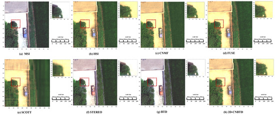
Figure 12.
Plot of fusion results of UAV acquisition of Qingtongxia rice field dataset.
The assessment of the compared algorithms is shown in Table 5, and the better experimental results are indicated in bold. In terms of the spatial spectral characteristics, the algorithms in this paper and FUSE are closer to 1 for SSIM, UIQI, and CC values, and closer to 0 for RMSE, ERGAS, and SAM, indicating that the fused images have minimal spectral distortion and better spatial structure. In comparison, the algorithm in this paper is better than FUSE. The algorithm in this paper has the highest PSNR, which indicates that the algorithm in this paper can eliminate noise well. The running time of the algorithm is slightly longer.
Table 5.
Performance for UAV acquisition of Qingtongxia rice field.
4.9. Discussion
The superiority and applicability of the fusion algorithm is mainly demonstrated by the results on different datasets.
As shown in Figure 9 and Figure 10, in the standard dataset test, CNMF lost part of the spatial details in Figure 9, and there was serious spectral distortion in Figure 10. Hysure, STEREO, and BTD algorithms had better fusion results in Figure 9, with a lower loss of spectral and spatial information, and only a small amount of blurred blocks existing in the images. In Figure 10, all three algorithms had poor fusion results, with a large number of blurred blocks in the images, indicating that in the Indian Pine dataset, the three algorithms lose a large amount of spectral and spatial information in the fusion process, and BTD is particularly serious. In Figure 9 and Figure 10, the FUSE algorithm has a small number of blurred blocks in the fusion results. In Figure 9 and Figure 10, SCOTT shows the worst fusion results, with a large number of blurred blocks and noise, and a serious loss of spatial–spectral information. In Figure 9 and Figure 10, the fusion results of the proposed algorithm in this paper are closest to the reference image, and the blurred blocks and noise in the images are small. In order to further verify the effectiveness of the fusion algorithm, the metrics for evaluating the spatial and spectral features were selected to describe the effectiveness of the algorithm (as shown in Table 2 and Table 3). The experimental results show that CNMF’s UIQI values in the Pavia University dataset and the SSIM values in the Indian Pine dataset are closer to the optimal values, indicating that CNMF is able to preserve the spatial information in the images. The SCOTT algorithm has poor evaluation metrics on both standard datasets, Hysure and FUSE have better evaluation metrics on both datasets, and STEREO and BTD have moderate performance on the Pavia University dataset but poor performance on the Indian Pine dataset; Except for the UIQI value of the Pavia University dataset and the SSIM value of the Indian pine dataset, the results of other metrics show that the algorithm in this paper is closer to the optimal value.
As shown in Figure 11 and Figure 12, in the local dataset test, CNMF has misalignment, fuzzy blocks, and spectral distortion in the fusion results in Figure 11, and larger fuzzy blocks in the fusion results in Figure 12. FUSE and BTD have clear fusion results in Figure 11 and smaller blurred blocks in the fusion results in Figure 12. SCOTT has serious noise, misalignment, and loss of spatial and spectral information in the fusion results in both Figure 11 and Figure 12. STEREO has severe spectral distortion and a large amount of noise in the fusion results in Figure 11, and large blurred blocks in the fusion results in Figure 12. The algorithm in this paper has clear spatial textures in the fusion results of Figure 11 and Figure 12, and there is no distortion, blurred blocks or other phenomena. In order to further verify the effectiveness of the fusion algorithm, the indexes for evaluating the spatial features and spectral features are selected to describe the effectiveness of the algorithm (as shown in Table 4 and Table 5). The experimental results show that the evaluation indexes of CNMF, SCOTT, STEREO, and BTD on the local dataset perform poorly in general. The evaluation indexes of FUSE on the local dataset perform moderately. The evaluation indexes of the algorithm in this paper on the local dataset are closer to the optimal value.
In summary, CNMF and STEREO show spectral distortion and misalignment in some dataset tests. The SCOTT, STEREO, and BTD algorithms show a large number of fuzzy blocks and noisy situations, indicating that CNMF, SCOTT, and other algorithms show a loss of spatial and spectral information in the process of fusion, and that the algorithms are less applicable scenes. The algorithm proposed in this paper performs better on both standard and local datasets, and the HRHS image texture information is clear, relatively smooth, and closer to the reference image, indicating that it can well retain the spectral information and spatial structure of the image in the fusion process, and that the algorithm can be applied to a variety of scenes.
5. Conclusions
A coupled non-negative block-term tensor decomposition model based on regularization is used to estimate HRHS. Considering the sparsity and smoothness of the endmember matrix and the abundance matrix, the norm is introduced to describe its sparsity. In addition, the difference operators in the horizontal and vertical directions are defined and introduced into the model to describe the segmental smoothness. Finally, the proposed model is solved using two optimization algorithms, ADMM and PAO. Experimental validation on real and local datasets shows that there is a slight difference with the CNMF algorithm in the spatial feature indexes UIQI and SSIM, but the overall performance is excellent in spectral information feature indexes. Further, it is confirmed that the spatial and spectral features of the fusion results of the algorithm in this paper remain consistent with the reference image.
The proposed algorithm in this paper has a minor limitation because the norm has a non-smooth feature, which is not the best choice for the sparse endmember matrix and abundance matrix, and the algorithm running time is slightly longer due to the tensor rank estimation. In future work, it can be extended in these two directions; firstly, by considering other means to promote the sparsity of the abundance and endmember matrices, and secondly, to reduce the algorithm running time without affecting the performance of the MHF algorithm.
Author Contributions
Funding acquisition, W.B.; Validation, K.Q.; Writing—original draft, H.G.; Writing—review and editing, H.G., W.B., K.Q., X.M. and M.C. All authors have read and agreed to the published version of the manuscript.
Funding
This work is supported by the Natural Science Foundation of Ningxia Province of China (Project No. 2020AAC02028), the Natural Science Foundation of Ningxia Province of China (Project No. 2021AAC03179), and the National Natural Science Foundation of China (Project No. 62201438).
Data Availability Statement
Publicly available datasets were analyzed in this study. This data can be found here: https://www.ehu.eus/ccwintco/index.php?title=Hyperspectral_Remote_Sensing_Scenes, 1 September 2022.
Acknowledgments
The authors thank the reviewers for their critiques and comments. The authors would like to thank the Key Laboratory of Images and Graphics Intelligent Processing of the State Ethnic Affairs Commission (IGIPLab) for their support. At the same time, authors would like to thank Xiao Fu, Guoyong Zhang, and Meng Ding for their help, and for sharing the MATLAB code on block-term tensor decomposition.
Conflicts of Interest
The authors declare no conflict of interest.
Abbreviations
The following abbreviations are used in this manuscript:
| MHF | Multispectral and hyperspectral image fusion |
| HRHS | High spatial resolution hyperspectral images |
| HSI | Hyperspectral images |
| MSI | Multispectral images |
| LR-HSI | Low-resolution hyperspectral images |
| HR-MSI | High-resolution multispectral images |
| HSR | Hyperspectral super-resolution |
| PAN | Panchromatic images |
| CPD | Canonical polyadic decomposition |
| TV | Total variational |
| PAO | Proximal alternating optimization |
| ADMM | Alternating directional multiplier method |
| SNRs | Signal-to-noise ratios |
| PCA | Principal component analysis |
| PSNR | Peak signal to noise ratio |
| SSIM | Structural similarity |
| CC | Correlation coefficient |
| UIQI | Universal image quality index |
| RMSE | Root mean squared error |
| ERGAS | Erreur Relative Globale Adimensionnelle De Synthese |
| SAM | Spectral angle mapper |
Appendix A
Symbol Definition
Bold lowercase and uppercase characters are used to represent vectors and matrices, separately. The upper-order tensor is represented by . For a tensor , a denotes its n-order expansion. ⊗ denotes the Kronecker product. The Khatri-Rao product is indicated by ⊙ in its ordinary version. Denote by the Khatri-Rao column form. ∘ denotes the outer product. The unit matrix of nth order is denoted by . denotes the complex number field.
Appendix B
Appendix B.1. Optimization Problem on B
Fixing A, and C, the optimization problem on B in the above equation is shown as follows.
By means of the mode-2 expansion and introducing the splitting variable , problem (A1) can be reformulated as:
where and is obtained by matrixing Equation (6) to obtain the augmented Lagrangian function for problem (A2).
where is the Lagrangian multiplier and is the positive penalized parameter.
For problem (A3), the ADMM iterative equation is shown below:
In the following, the solution procedure of problem (A4) is given.
- Subproblem of B: For problem (A3), the minimization objective function is as follows:Problem (A5) is a quadratic optimization problem whose solution is unique. Compute Sylvester’s equation to solve B by calculating the following, i.e.:In this paper, this problem is effectively solved by using CG [44].
- Subproblem of : For problem (A3), the minimization objective function is as follows:The solution of its is well known as a soft threshold, i.e.:
- Subproblem of : For problem (A3), the updated Lagrange multiplier is given by:
The pseudo-code of the optimization algorithm on B is shown in Algorithm A1.
| Algorithm A1 Solving B-Subproblem (A3) via ADMM. |
| Input, , , , , , , , . |
| Output Dictionary matrix B |
| While unconverged do |
| Updating the matrix B by solving problem (A4) with the CG method; |
| Updating the variable by ); |
| Updating the Lagrangian multiplier L2 by L2 − (DHB − U2); |
| end While |
Appendix B.2. Optimization Problem on C
Fixing A, B, the optimization problem on C in the above equation is shown as follows.
By means of the mode-3 expansion and introducing the splitting variable , problem (A10) can be reformulated as:
where and is obtained using matrix Equation (7) to obtain the augmented Lagrangian function for problem (A11).
where is the Lagrangian multiplier and is the positive penalized parameter.
For problem (A12), the ADMM iterative equation is shown below:
In the following, the solution procedure of problem (A13) is given.
- Subproblem of C: For problem (A12), the minimization objective function is as follows:Problem (A14) is a quadratic optimization problem whose solution is unique. Compute Sylvester’s equation to solve C by calculating the following, i.e.:This problem is effectively solved by using CG [44] in this paper.
- Subproblem of : For problem (A12), the minimization objective function is as follows:The solution of its is well known as a soft threshold, i.e.:
- Subproblem of : For problem (A12), the updated Lagrange multiplier is given by:
The pseudo-code of the optimization algorithm on C is shown in Algorithm A2.
| Algorithm A2 Solving C-Subproblem (A12) via ADMM. |
| Input, , , , ,, , , . |
| Output Dictionary matrix C |
| While unconverged do |
| Updating the matrix C by solving problem (A14) with the CG method; |
| Updating the variable by ); |
| Updating the Lagrangian multiplier L3 by L3 − ( DHC − U3); |
| end While |
References
- Cao, M.; Bao, W.; Qu, K. Hyperspectral super-resolution via joint regularization of low-rank tensor decomposition. Remote Sens. 2021, 13, 4116. [Google Scholar] [CrossRef]
- Loncan, L.; Almeida, L.B.D.; Bioucas-Dias, J.M.; Briottet, X.; Chanussot, J.; Dobigeon, N.; Fabre, S.; Liao, W.; Licciardi, G.A.; Simoes, M.; et al. Hyperspectral pansharpening: A review. IEEE Geosci. Remote Sens. Mag. 2015, 3, 27–46. [Google Scholar] [CrossRef]
- Meng, X.; Shen, H.; Li, H.; Zhang, L.; Fu, R. Review of the pansharpening methods for remote sensing images based on the idea of meta-analysis: Practical discussion and challenges. Inf. Fusion 2019, 46, 102–113. [Google Scholar] [CrossRef]
- Carper, W.; Lillesand, T.; Kiefer, R. The use of intensity-hue-saturation transformations for merging spot panchromatic and multispectral image data. Photogramm. Eng. Remote Sens. 1990, 56, 459–467. [Google Scholar]
- Aiazzi, B.; Baronti, S.; Selva, M. Improving component substitution pansharpening through multivariate regression of ms + pan data. IEEE Trans. Geosci. Remote Sens. 2007, 45, 3230–3239. [Google Scholar] [CrossRef]
- Liu, J. Smoothing filter-based intensity modulation: A spectral preserve image fusion technique for improving spatial details. Int. J. Remote Sens. 2000, 21, 3461–3472. [Google Scholar] [CrossRef]
- Aiazzi, B.; Alparone, L.; Baronti, S.; Garzelli, A.; Selva, M. An mtf-based spectral distortion minimizing model for pan-sharpening of very high resolution multispectral images of urban areas. In Proceedings of the 2003 2nd GRSS/ISPRS Joint Workshop on Remote Sensing and Data Fusion over Urban Areas, Berlin, Germany, 22–23 May 2003; pp. 90–94. [Google Scholar]
- Vivone, G.; Alparone, L.; Chanussot, J.; Mura, M.D.; Garzelli, A.; Licciardi, G.A.; Restaino, R.; Wald, L. A critical comparison among pansharpening algorithms. IEEE Trans. Geosci. Remote Sens. 2014, 53, 2565–2586. [Google Scholar] [CrossRef]
- Gomez, R.B.; Jazaeri, A.; Kafatos, M. Wavelet-based hyperspectral and multispectral image fusion. In Geo-Spatial Image and Data Exploitation II; SPIE: Washington, DC, USA, 2001; Volume 4383, pp. 36–42. [Google Scholar]
- Zhang, Y.; He, M. Multi-spectral and hyperspectral image fusion using 3-d wavelet transform. J. Electron. 2007, 24, 218–224. [Google Scholar] [CrossRef]
- Leung, Y.; Liu, J.; Zhang, J. An improved adaptive intensity–hue–saturation method for the fusion of remote sensing images. IEEE Geosci. Remote Sens. Lett. 2013, 11, 985–989. [Google Scholar] [CrossRef]
- Kwarteng, P.; Chavez, A. Extracting spectral contrast in landsat thematic mapper image data using selective principal component analysis. Photogramm. Eng. Remote Sens. 1989, 55, 339–348. [Google Scholar]
- Li, H.; Manjunath, B.; Mitra, S.K. Multisensor image fusion using the wavelet transform. Graph. Model. Image Process. 1995, 57, 235–245. [Google Scholar] [CrossRef]
- Selva, M.; Aiazzi, B.; Butera, F.; Chiarantini, L.; Baronti, S. Hyper-sharpening: A first approach on sim-ga data. IEEE J. Sel. Top. Appl. Earth Obs. Remote Sens. 2015, 8, 3008–3024. [Google Scholar] [CrossRef]
- Yokoya, N.; Grohnfeldt, C.; Chanussot, J. Hyperspectral and multispectral data fusion: A comparative review of the recent literature. IEEE Geosci. Remote Sens. Mag. 2017, 5, 29–56. [Google Scholar] [CrossRef]
- Yokoya, N.; Yairi, T.; Iwasaki, A. Coupled nonnegative matrix factorization unmixing for hyperspectral and multispectral data fusion. IEEE Trans. Geosci. Remote Sens. 2011, 50, 528–537. [Google Scholar] [CrossRef]
- Bendoumi, M.A.; He, M.; Mei, S. Hyperspectral image resolution enhancement using high-resolution multispectral image based on spectral unmixing. IEEE Trans. Geosci. Remote Sens. 2014, 52, 6574–6583. [Google Scholar] [CrossRef]
- Berné, O.; Helens, A.; Pilleri, P.; Joblin, C. Non-negative matrix factorization pansharpening of hyperspectral data: An application to mid-infrared astronomy. In Proceedings of the 2010 2nd Workshop on Hyperspectral Image and Signal Processing: Evolution in Remote Sensing, Reykjavik, Iceland, 14–16 June 2010; pp. 1–4. [Google Scholar]
- Simoes, M.; Bioucas-Dias, J.; Almeida, L.B.; Chanussot, J. A convex formulation for hyperspectral image superresolution via subspace-based regularization. IEEE Trans. Geosci. Remote Sens. 2014, 53, 3373–3388. [Google Scholar] [CrossRef]
- Wei, Q.; Dobigeon, N.; Tourneret, J.-Y. Fast fusion of multi-band images based on solving a sylvester equation. IEEE Trans. Image Process. 2015, 24, 4109–4121. [Google Scholar] [CrossRef]
- Wei, Q.; Bioucas-Dias, J.; Dobigeon, N.; Tourneret, J.-Y. Hyperspectral and multispectral image fusion based on a sparse representation. IEEE Trans. Geosci. Remote Sens. 2015, 53, 3658–3668. [Google Scholar] [CrossRef]
- Veganzones, M.A.; Simoes, M.; Licciardi, G.; Yokoya, N.; Bioucas-Dias, J.M.; Chanussot, J. Hyperspectral super-resolution of locally low rank images from complementary multisource data. IEEE Trans. Image Process. 2015, 25, 274–288. [Google Scholar] [CrossRef]
- Prévost, C.; Usevich, K.; Comon, P.; Brie, D. Hyperspectral super-resolution with coupled tucker approximation: Recoverability and svd-based algorithms. IEEE Trans. Signal Process. 2020, 68, 931–946. [Google Scholar] [CrossRef]
- Dian, R.; Fang, L.; Li, S. Hyperspectral image super-resolution via non-local sparse tensor factorization. In Proceedings of the IEEE Conference on Computer Vision and Pattern Recognition, Honolulu, HI, USA, 21–26 July 2017; pp. 5344–5353. [Google Scholar]
- Xu, T.; Huang, T.-Z.; Deng, L.-J.; Zhao, X.-L.; Huang, J. Hyperspectral image superresolution using unidirectional total variation with tucker decomposition. IEEE J. Sel. Top. Appl. Earth Obs. Remote Sens. 2020, 13, 4381–4398. [Google Scholar] [CrossRef]
- Li, S.; Dian, R.; Fang, L.; Bioucas-Dias, J.M. Fusing hyperspectral and multispectral images via coupled sparse tensor factorization. IEEE Trans. Image Process. 2018, 27, 4118–4130. [Google Scholar] [CrossRef] [PubMed]
- Zhang, K.; Wang, M.; Yang, S. Multispectral and hyperspectral image fusion based on group spectral embedding and low-rank factorization. IEEE Trans. Geosci. Remote Sens. 2016, 55, 1363–1371. [Google Scholar] [CrossRef]
- Li, W.; Du, Q. A survey on representation-based classification and detection in hyperspectral remote sensing imagery. Pattern Recognit. Lett. 2016, 83, 115–123. [Google Scholar] [CrossRef]
- Zhang, K.; Wang, M.; Yang, S.; Jiao, L. Spatial–spectral-graph-regularized low-rank tensor decomposition for multispectral and hyperspectral image fusion. IEEE J. Sel. Top. Appl. Earth Obs. Remote Sens. 2018, 11, 1030–1040. [Google Scholar] [CrossRef]
- Li, Q.; Ma, W.-K.; Wu, Q. Hyperspectral super-resolution: Exact recovery in polynomial time. In Proceedings of the 2018 IEEE Statistical Signal Processing Workshop (SSP), Freiburg im Breisgau, Germany, 10–13 June 2018; pp. 378–382. [Google Scholar]
- Kanatsoulis, C.I.; Fu, X.; Sidiropoulos, N.D.; Ma, W.-K. Hyperspectral super-resolution: A coupled tensor factorization approach. IEEE Trans. Signal Process. 2018, 66, 6503–6517. [Google Scholar] [CrossRef]
- Zhang, G.; Fu, X.; Huang, K.; Wang, J. Hyperspectral super-resolution: A coupled nonnegative block-term tensor decomposition approach. In Proceedings of the 2019 IEEE 8th International Workshop on Computational Advances in Multi-Sensor Adaptive Processing (CAMSAP), Le gosier, Guadeloupe, 15–18 December 2019; pp. 470–474. [Google Scholar]
- Lathauwer, L.D. Decompositions of a higher-order tensor in block terms—Part i: Lemmas for partitioned matrices. SIAM J. Matrix Anal. Appl. 2008, 30, 1022–1032. [Google Scholar] [CrossRef]
- Lathauwer, L.D. Decompositions of a higher-order tensor in block terms—Part ii: Definitions and uniqueness. SIAM J. Matrix Anal. Appl. 2008, 30, 1033–1066. [Google Scholar] [CrossRef]
- De Lathauwer, L.; Nion, D. Decompositions of a higher-order tensor in block terms—Part iii: Alternating least squares algorithms. SIAM J. Matrix Anal. Appl. 2008, 30, 1067–1083. [Google Scholar] [CrossRef]
- Ding, M.; Fu, X.; Huang, T.-Z.; Wang, J.; Zhao, X.-L. Hyperspectral super-resolution via interpretable block-term tensor modeling. IEEE J. Sel. Top. Signal Process. 2020, 15, 641–656. [Google Scholar] [CrossRef]
- Hitchcock, F.L. The expression of a tensor or a polyadic as a sum of products. J. Math. Phys. 1927, 6, 164–189. [Google Scholar] [CrossRef]
- Tucker, L.R. Some mathematical notes on three-mode factor analysis. Psychometrika 1966, 31, 279–311. [Google Scholar] [CrossRef] [PubMed]
- Zeng, Z.-Y.; Huang, T.-Z.; Chen, Y.; Zhao, X.-L. Nonlocal block-term decomposition for hyperspectral image mixed noise removal. IEEE J. Sel. Top. Appl. Earth Obs. Remote Sens. 2021, 14, 5406–5420. [Google Scholar] [CrossRef]
- Ma, W.-K.; Bioucas-Dias, J.M.; Chan, T.-H.; Gillis, N.; Gader, P.; Plaza, A.J.; Ambikapathi, A.; Chi, C.-Y. A signal processing perspective on hyperspectral unmixing: Insights from remote sensing. IEEE Signal Process. Mag. 2013, 31, 67–81. [Google Scholar] [CrossRef]
- Wycoff, E.; Chan, T.-H.; Jia, K.; Ma, W.-K.; Ma, Y. A non-negative sparse promoting algorithm for high resolution hyperspectral imaging. In Proceedings of the 2013 IEEE International Conference on Acoustics, Speech and Signal Processing, Vancouver, BC, Canada, 26–31 May 2013; pp. 1409–1413. [Google Scholar]
- Attouch, H.; Bolte, J.; Svaiter, B.F. Convergence of descent methods for semi-algebraic and tame problems: Proximal algorithms, forward–backward splitting, and regularized gauss–seidel methods. Math. Program. 2013, 137, 91–129. [Google Scholar] [CrossRef]
- Attouch, H.; Bolte, J.; Redont, P.; Soubeyran, A. Proximal alternating minimization and projection methods for nonconvex problems: An approach based on the kurdyka-łojasiewicz inequality. Math. Oper. Res. 2010, 35, 438–457. [Google Scholar] [CrossRef]
- Liu, J.S.; Chen, R. Sequential monte carlo methods for dynamic systems. J. Am. Stat. Assoc. 1998, 93, 1032–1044. [Google Scholar] [CrossRef]
- Sui, L.; Li, L.; Li, J.; Chen, N.; Jiao, Y. Fusion of hyperspectral and multispectral images based on a bayesian nonparametric approach. IEEE J. Sel. Top. Appl. Earth Obs. Remote Sens. 2019, 12, 1205–1218. [Google Scholar] [CrossRef]
- Wang, Z.; Bovik, A.C. A universal image quality index. IEEE Signal Process. Lett. 2002, 9, 81–84. [Google Scholar] [CrossRef]
- Wald, L. Quality of high resolution synthesised images: Is there a simple criterion? In Proceedings of the Third Conference “Fusion of Earth Data: Merging Point Measurements, Raster Maps and Remotely Sensed Images” SEE/URISCA, Sophia Antipolis, France, 26 January 2000; pp. 99–103. [Google Scholar]
- Yuhas, R.H.; Goetz, A.F.; Boardman, J.W. Discrimination among semi-arid landscape endmembers using the spectral angle mapper (sam) algorithm. In Proceedings of the JPL, Summaries of the Third Annual JPL Airborne Geoscience Workshop, Volume 1: AVIRIS Workshop, Pasadena, CA, USA, 23–26 January 1992; pp. 147–149. [Google Scholar]
- Bioucas-Dias, J.M.; Plaza, A.; Dobigeon, N.; Parente, M.; Du, Q.; Gader, P.; Chanussot, J. Hyperspectral unmixing overview: Geometrical, statistical, and sparse regression-based approaches. IEEE J. Sel. Top. Appl. Earth Obs. Remote Sens. 2012, 5, 354–379. [Google Scholar] [CrossRef]


Publisher’s Note: MDPI stays neutral with regard to jurisdictional claims in published maps and institutional affiliations. |
© 2022 by the authors. Licensee MDPI, Basel, Switzerland. This article is an open access article distributed under the terms and conditions of the Creative Commons Attribution (CC BY) license (https://creativecommons.org/licenses/by/4.0/).