Abstract
Radar data assimilation has been operational at the Deutscher Wetterdienst for several years and is essential for generating accurate precipitation forecasts. The current work attempts to further enhance the radar data assimilation by improving the latent heat nudging (LHN) scheme and by reducing the observation error (OE) caused by the representation error of the efficient modular volume radar operator (EMVORADO). First of all, a series of hindcasts for a one-month convective period over Germany are performed. Compared with radar reflectivity and satellite observations, it is found that the LHN scheme that implicitly adjusts temperature performs better, and the beam broadening effect and the choice of the scattering schemes in EMVORADO are important. Moreover, the Mie scheme with the new parameterization to reduce the brightband effect not only proves to be the best in hindcasts but also that it results in the smallest standard deviations and the shortest horizontal correlation length scales of the OE in data assimilation experiments.
1. Introduction
Since February 2021, the convection-permitting isosahedral non-hydrostatic Deutschland (Germany) 2 (ICON-D2) horizontal grid spacing of 2 km) model has been operational for short-range forecasts at the Deutscher Wetterdienst (DWD, Germany’s National Meteorological Service). Initial conditions are provided by the kilometre-scale ensemble data assimilation (KENDA) [1]) system, in which the local ensemble transform Kalman filter (LETKF [2]) scheme is implemented to assimilate conventional observations as well as remote sensing data, e.g., satellite and weather radar data (including 3D volume-scanning reflectivity and radial wind data). In addition, the latent heat nudging (LHN [3]) is employed to assimilate radar-derived surface precipitation rates. Since the KENDA system has become operational, continuous efforts have been made to improve it. The current study focuses on how to enhance the performance of the radar data assimilation, in which two aspects are of particular interest. First, the LHN schemes could be associated with the imbalance (also called “ramp-down” [4]) issue, i.e., the model is nudged toward observations too strongly and shocks could be introduced to model (thermo)dynamics, which therefore could cause a rapid loss of forecast skills. Secondly, Zeng et al. [5] used the ICON-D2-KENDA with the efficient modular volume radar operator (EMVORADO [6,7,8,9,10]) to investigate observation error statistics of reflectivity and radial wind. It is found that representation error in the radar forward operator (hereafter denoted by “FE”) caused by neglecting the effects of reflectivity weighting or terminal fall speed of hydrometeors is omittable by average, but the FE due to neglecting the beam broadening effect as well as due to the scattering schemes can be significant. For instance, the Mie scheme with a specific parameterization for melting particles results in a considerably larger FE around the melting layer than the Rayleigh scheme. This could be due to the inappropriate parameterization, but this could also be associated with the strong nonlinearity of the Mie scattering scheme that the LETKF cannot cope with well.
In this work, first of all, we attempt to obtain an easier and better understanding of the impacts of the LHN schemes as well as impacts of configurations of EMVORADO (e.g., the beam broadening effect and the scattering schemes) by performing a series of hindcasting experiments with ICON-D2 for a summer period over Germany, without possible mutual influences with the data assimilation. A similar study has been conducted by Geiss et al. [11] but for tuning the novel visible satellite image forward operator (VISOP) that extends the method for fast satellite image simulation (MFASIS) for 1D radiative transfer [12] to account for most important 3D radiative transfer effects [13]. By analysing results of hindcasts, it may in turn help us refine the KENDA system. Therefore, in the second half of this work, a series of data assimilation experiments with different configurations of EMVORADO are executed, based on the KENDA system. The statistics of the OE are then estimated by the Desroziers method [14], aiming to explore whether improved configurations of EMVORADO indicated by the hindcasts also reduce the FE and consequently OE in data assimilation.
The paper is organized as follows. Section 2 briefly introduces ICON-D2 and observations that are used to validate the performance of hindcasts, and proposes two different LHN schemes and describes the Desroziers method. Section 3 and Section 4 describe the experimental designs and results for hindcasts and data assimilation, respectively. Section 5 gives the summary and outlook.
2. Model, Observations, and Methodology
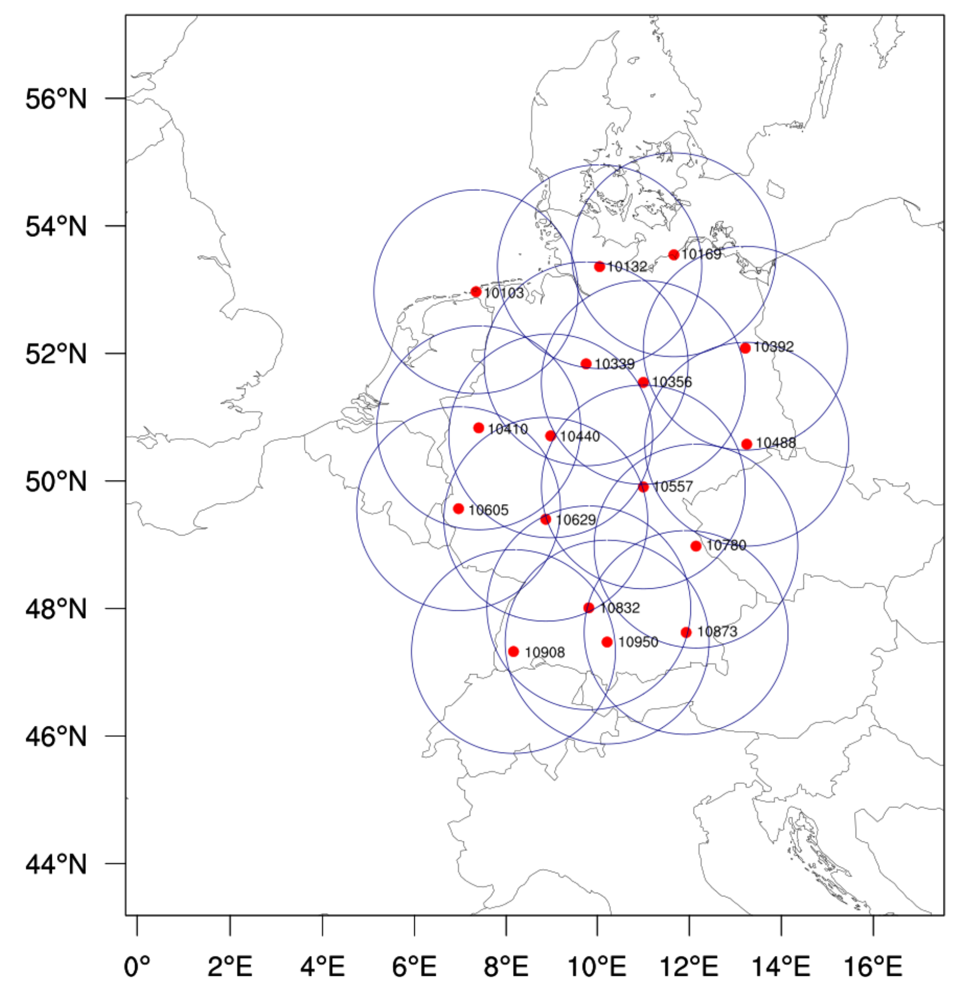
ICON-D2, the regional model of the German weather service is used in this study. It has a horizontal resolution of 2 km and 65 vertical levels, and its domain covers Germany and some parts of neighboring nations (see Figure 1). ICON-D2 is initialized by downscaled ICON-EU analysis and is hourly driven by analysis lateral boundary conditions from the ICON-EU (one-way nesting). The one-moment bulk microphysical scheme for cloud ice , cloud droplets , snow , rain , and graupel is used [15,16]. In addition, the turbulence is parametrized by the scheme of Raschendorfer [17] and the shallow convection is parametrized by the scheme of Tiedtke [18], and the deep convection is explicitly resolved.

Figure 1.
Illustration of the ICON-D2 domain with the radar network of the DWD (each station is denoted by a red bullet with a station number, the scanning range is denoted by a circle).
The DWD operates a C-band Doppler radar network of 17 stations (distributed throughout Germany) with a uniform scan strategy that takes about 5 min to be completed. The scan begins with the terrain-following precipitation scan (horizontal range: 150 km), followed by the volume scan which starts with six consecutive antenna rotations for elevations of 5.5°, 4.5°, 3.5°, 2.5°, 1.5°, and 0.5° (horizontal range: 180 km) and then does another four rotations for elevations of 8.0°, 12.0°, 17.0°, and 25.0° (horizontal ranges decreasing from 160 km to 120 km as elevations increase). Based on five categorized empirical reflectivity-rainfall (Z–R) relationships that depend on the meteorological situations [3], precipitation rates are derived from reflectivity obtained by the precipitation scan.
To validate model outputs with radar reflectivity, EMVORADO is used to produce synthetic radar reflectivity, which is one of the most comprehensive radar forward operators utilized in operational suites (i.e., for each physical process, it provides different options associated with different accuracies and costs). For instance, for the beam broadening effect, EMVORADO provides the possibility of taking the varying beam width into account by using a certain amount of auxiliary rays in horizontal and vertical directions (relative to the beam axis), and the pulse-volume integration is performed over nodes given by the numerical Gauss–Legendre quadrature. For scattering schemes, there are two methods available, namely the Rayleigh method for (near-)spherical particles with relatively small sizes compared to the wavelength and the Mie method for one- or two-layered spherical particles with arbitrary sizes. For the former one, only one effective medium approximation (EMA) approach, namely the Oguchi-model [19] is implemented for calculating partially melted particles, which allows for analytic solutions. For the latter one, two EMA approaches, namely the Maxwell–Garnett and Bruggemann models [20,21], are implemented, which allows for the tuning for the melting layer, depending on the melting state and the particle morphology [9]. For detailed descriptions of the EMVORADO (e.g., equations for simulating reflectivity and radial wind), readers are referred to [5]. In order to validate the impacts of LHN schemes, VISOP and RTTOV are [22] additionally used to provide synthetic satellite data. As in [11], we use the visible 0.6 m channel (VIS006, simulated by VISOP), which usually has relatively smaller errors in the surface albedo, and the 10.8 m thermal infrared window channel (IR108, simulated by RTTOV), whose signals are in large part determined by the emission from the ground and clouds (only slightly affected by gaseous absorption).
The general concept of the LHN schemes assume that the surface precipitation rate at one grid point is proportional to the column-integrated latent heat, based on which the vertical profiles of (positive) temperature increments are generated. In this work, two LHN schemes are employed. In the first one (denoted by “LHN1”), temperature increments are generated based on the prognostic precipitation [3]; additionally, is adapted to accordingly, so that the relative humidity remains unchanged. In the second one (denoted by “LHN2”), is only used to derive and then is set to zero. The modifications to T are eventually realized via the saturation adjustment due to the increasing . Consequently, is generated over the whole column for the LHN1, whereas are only available at points with occurrence of the saturation adjustment for the LHN2. Therefore, the LHN2 is considered as an implicit approach to adjust T. The LHN schemes are applied continuously during the integration of the model by using data linearly interpolated in time between two consecutive observed precipitation rate fields.
The Desroziers method [14] is commonly used to estimate the observation error covariance matrix as
where and are background and analysis departures, and is the observation vector. Theoretically, the Desroziers method is an iterative process; however, in practice, the estimation of one iteration is often used due to its sufficient accuracy and low computational expense [23,24,25,26]), as in this work.
3. Results
3.1. Experimental Design
Similar to Geiss et al. [11], to obtain robust statistics, a one-month period from 1 June to 30 June 2020 with high occurrence of convection is chosen, characterized by the typical changeable central European summer weather. In particular, between 10 and 20 June, the sultry hot air caused thunderstorms with heavy showers often developed in a low-pressure trough, which was situated on a diagonal (from the northwest to the southeast) over Germany. Precipitation in this month amounted to approximately 90 mm, which was slightly higher than its long-term average of 85 mm for June. Overall, the length of the period and the size of the domain size are sufficient for the model to develop its own convection distribution.
In order to investigate the impacts of the LHN schemes and different configurations of EMVORADO, six different hindcasting experiments are performed with ICON-D2, hourly driven by the lateral boundary conditions throughout the one-month convective period described above. The goal of the first three ones is to investigate the performance of LHN schemes. For comparison, a control run without using any LHN schemes is done. The other three hindcasts are used to evaluate the different configurations of the EMVORADO, by which it is straightforward to see the representation error caused by the EMVORADO, not influenced by the LETKF algorithm or by the settings of the KENDA system. For instance, to evaluate the impacts of the beam broadening effect, E_mie1_lhn2 is compared to E_mie1_lhn2_bb, while the latter one accounts for the beam broadening effect with five auxiliary rays in the vertical direction (the horizontal direction is omitted because its impacts are insignificant [5]). To evaluate impacts of different scattering schemes and EMA approaches, E_mie1_lhn2_bb, E_ray_lhn2_bb and E_mie2_lhn2_bb are compared. E_ray_lhn2_bb employs the Rayleigh method (with the Oguchi-model for melting particles). Both E_mie1_lhn2_bb and E_mie2_lhn2_bb employ the Mie method; the latter one uses the Maxwell–Garnett model with a new parameterization, which includes increasing the starting melting temperature from 263.160 to 270.16 K to lower the height of the melting layer, decreasing the melting degree from 0.2 to 0.1 to abbreviate the refraction index and using “maisms” instead of “mawsms” for the particle morphology to shrink the size of particles. All of these contribute to the reduction of the brightband effect. Experimental setups are given in Table 1. It is noted that the use of the forward operators EMVORADO, VISOP, and RTTOV allows for direct comparison of radar and satellite observations with their corresponding synthetic observations.

Table 1.
Experimental setups: ✓ means “on” or “applicable” and × means “off” or “not applicable”.
3.2. Verification Method
In this work, experimental results are evaluated primarily in terms of the contoured frequency by altitude diagrams (CFADs [27]). Based on the 3D volume scanning data of the radar network for the entire one-month period, the CFADs for observed and simulated reflectivities are constructed. Additionally, In order to analyse cloud statistics, pseudo CFADs combining two satellite channels (i.e., brightness temperature (denoted by “”) of IR108) and solar reflectance (denoted by “R”) of VIS006) are constructed as in Geiss et al. [11], in which is referred to as height. For clouds with are considered as low clouds, as middle clouds and as high clouds. In addition, depending on R, clouds are classified into clear-sky (), thin to intermediate clouds , and thick clouds .
3.3. Evaluation of the LHN Schemes
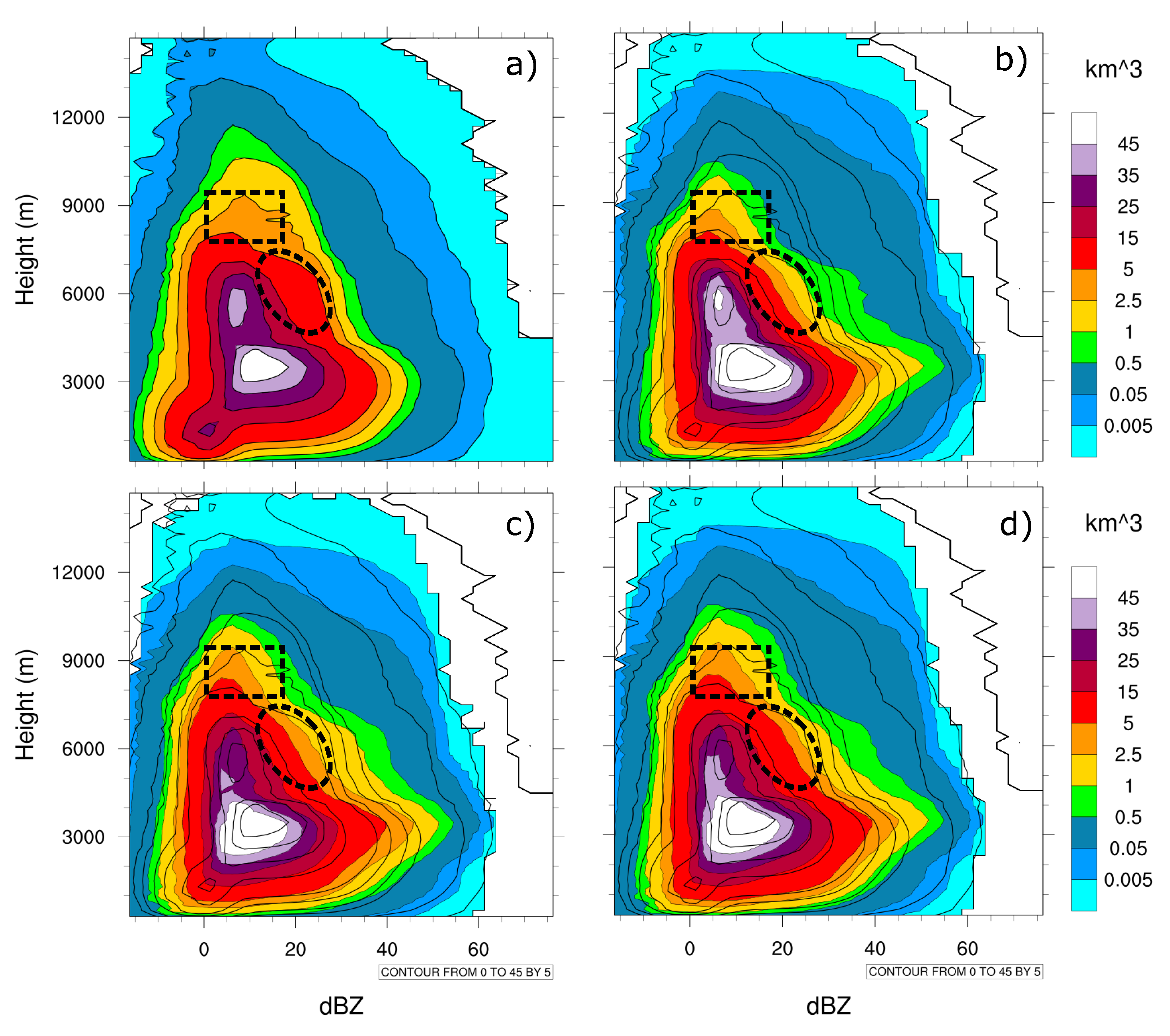
Figure 2 illustrates the CFADs of radar reflectivity for observations, E_mie1_nolhn, E_mie1_lhn1 and E_mie1_lhn2. In the observed CFAD (Figure 2a), broad distributions of reflectivity values occur at all heights, which is in line with Yuter and Houze [27] for the convective period. The highest frequencies can be seen for 10–20 dBZ around the melting layer (about 3 km high). Below the melting layer, reflectivity values with peak frequencies decrease rapidly with decreasing heights, probably due to evaporation. Reflectivity values dBZ are possibly caused by the raindrop collision/coalescence process and the melting large ice-phase particles. Above the melting layer, reflectivity values with peak frequencies decrease slowly with increasing heights. High reflectivity values (≥40 dBZ) indicate the existence of a considerable amount of graupel and hail, due to the riming of ice particles favored by convective updrafts. In contrast to observations, there are three clear differences in common among all experiments (Figure 2b–d): (1) Above 6 km, the amounts of reflectivities between 40 and 50 dBZ are prone to be overestimated but underestimated for reflectivities dBZ. As stated in Zeng et al. 2021c, the overestimation could be owing to the small slope intercept parameter for the graupel in the one-moment microphysical scheme; therefore, too much graupel with considerable sizes could be produced. The underestimation can be attributed to the model resolution (2 km) that may be not fine enough to resolve convective cores. The one-moment scheme utilized here could be another reason: as is known, reflectivity is proportional to (D particle size), which is in turn proportional to (q: mixing ratio; N: number concentration). In case of the one-moment scheme, larger q is coupled with larger N; therefore, it is not able to produce a few very large particles (here probably graupel). Below 4 km, the ground clutter effect can also contribute to very high observed reflectivities. (2) Reflectivities are considerably overestimated around the melting layer. (3) Fewer reflectivities are available above 12 km. For (1), one can consider using the two-moment instead of the one-moment scheme, but it is out of the scope of the current work. For (2) and (3), more discussion can be found in Section 3.4.

Figure 2.
The CFADs of radar reflectivity from 1 June to 1 July 2020 for (a) observations, (b) E_mie1_nolhn, and (c) E_mie1_lhn2. In calculations of the CFADS, in order to consider the beam broadening effect (i.e., pulse volume grows as distances increase), frequencies of reflectivities at further distances are multiplied with larger factors than those at shorter distances. Solid lines in (b–d) indicate contour lines of observations. Dashed line ellipses highlight impacts of the LHN scheme.
By comparing Figure 2b,c, the most remarkable differences between not using and using the LHN1 can be seen for reflectivity values 0–20 dBZ between heights 8 and 10 km (highlighted by dashed line squares). The LHN1 results in closer frequency distributions to observed ones as it either effectively extends the depth of convection or generates deep convection missing in the model. By comparing Figure 2c,d, frequency distributions of the LHN2 are closer to observed ones than those of the LHN1 for reflectivities 10–30 dBZ between heights 4 and 7 km (highlighted by dashed line ellipses). This could be because the LHN2 adjusts T in an implicit way that may mitigate the imbalance issue and may be more favorable for longer life cycles of convection.
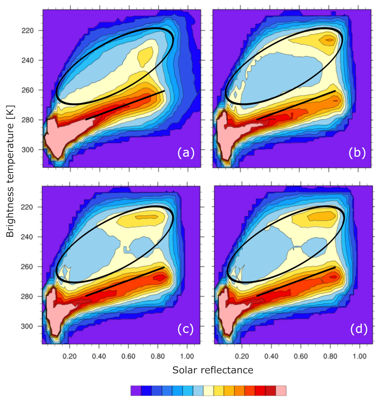
Furthermore, Figure 3 compares observations with experiments by means of pseudo CFADs that combine satellite channels of brightness temperature and solar reflectance (the former one is regarded as the height information). It is noticed in observations (Figure 3a) that the peak distributions occur for low and thin clouds, and the amounts of clouds decrease gradually with growing altitudes and cloud thickness. Compared to the observed pseudo CFADs, Figure 3b exhibits similar distributions on the whole; however, clear differences can be also seen. First, the slope of the BT-reflectance relation characterizing low-level clouds with reflectance between 0.3 and 0.9 (highlighted by solid lines) is steeper in Figure 3a than in Figure 3b, (in line with Geiss et al. [11]), which could indicate deficiencies in shallow convection parameterization of the model. Secondly, for middle clouds (highlighted by solid line ellipses), thin clouds at lower (higher) levels are underestimated (overestimated) for reflectance between 0.2 and 0.6, and a local peak centered at brightness temperature 240 K and reflectance 0.7 in the observed CFAD is shifted to 250 K and 0.8. The difficulty in representing middle clouds is a common problem in NWP models [28], likely due to systematic biases of models [29], caused, for instance, by a too active deep convection scheme. By using the LHN1 (see Figure 3c), the slope of the reflectance between 0.3 and 0.9 becomes a bit steeper and the overestimation of very thin clouds at the boundary layer is slightly corrected. The representation of middle clouds is considerably improved. For instance, the overestimation of thin clouds at higher levels is reduced and the center of the local peak moves slightly leftward (from 0.8 to 0.75). By using the LHN2 (see Figure 3d), no clear further improvements can be seen compared to the LHN1.

Figure 3.
The pseudo CFADS of reflectance from 1 June to 1 July 2020 for (a) observations, (b) E_mie1_nolhn, (c) E_mie1_lhn1, and (d) E_mie1_lhn2.
3.4. Evaluation of the Radar Forward Operator
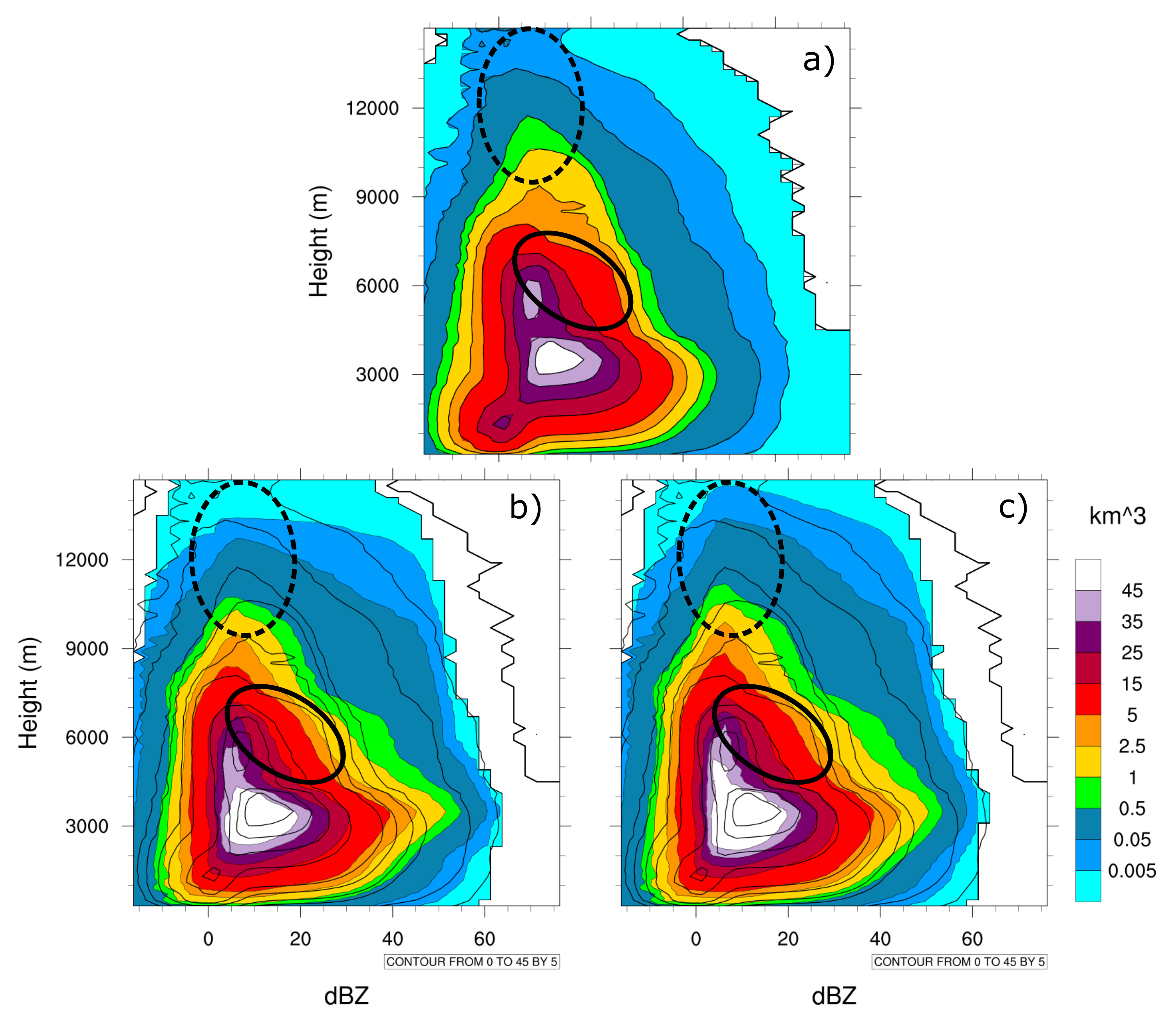
In order to show the impacts of accounting for the beam broadening effect, Figure 4 compares the CFAD of radar reflectivity observations with those of E_mie1_lhn2 and E_mie1_lhn2_bb. The most noticeable differences occur for reflectivity values 0–20 dBZ above 9 km (highlighted by dashed line ellipses), where probability distributions of E_mie1_lhn2_bb are considerably closer to observations. This is obviously due to the fact that the beam broadening effect becomes prominent as further distances (higher heights, accordingly) are reached. In addition, differences can be also seen for 0–30 dBZ between heights 4 and 7 km (highlighted by solid line ellipses). Because it is closer to the melting layer, this is likely caused by the beam interception of the melting layer, which leads to the pulse-volume averaging over inhomogeneous vertical profiles of reflectivity. Results are in line with the smaller FE of EMVORADO by accounting for the beam broadening effect in Zeng et al. [5].

Figure 4.
Same as Figure 2 but for (a) observations (b) E_mie1_lhn2, and (c) E_mie1_lhn2_bb.
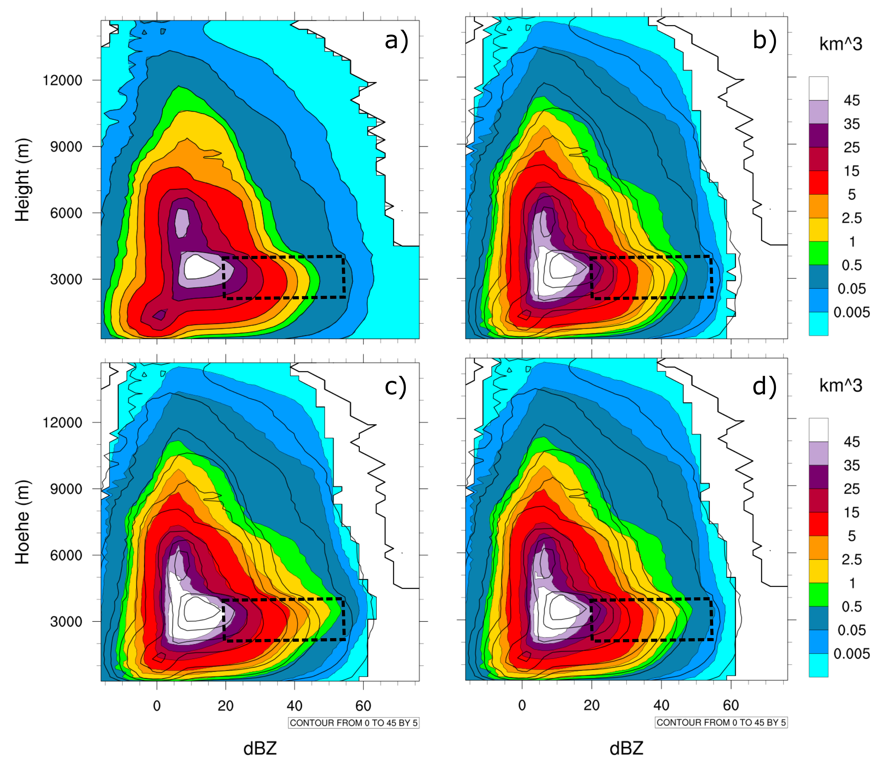
In order to show the impacts of scattering schemes and EMA approaches, Figure 5 compares the CFAD of radar reflectivity observations with those of E_mie1_lhn2_bb, E_ray_lhn2_bb, and E_mie2_lhn2_bb. It is easily recognized that reflectivity values are considerably overestimated around the melting layer in E_mie1_lhn2_bb, indicating that the parameterization for the the melting particles may not be appropriate. Smaller reflectivity values are produced at the melting layer by using the Rayleigh–Oguchi approximation in E_ray_lhn2_bb, which are much closer to observations. Results are consistent with the smaller FE of EMVORADO around the melting layer by using the Rayleigh–Oguchi approximation in [5]. However, in case of the Mie scheme, by using the new parameterization for the melting particles (see Section 3.1), the overestimation due the brightband effect is reduced in E_mie2_lhn2_bb, which results in a similar pattern as E_ray_lhn2_bb.

Figure 5.
Same as Figure 2 but for (a) observations (b) E_mie1_lhn2_bb (c) E_ray_lhn2_bb, and (d) E_mie2_lhn2_bb.
4. Experimental Design and Results of Data Assimilation
For data assimilation experiments, we use the ICON-LAM-KENDA system with the the LETKF and choose the convective period 10–15 June in 2020 (part of the specific period for hindcasts). As in previous studies [5,26], the assimilation window is one hour. The ensemble size is 40 and additionally a deterministic run is carried on. Observations include conventional data and radar data (reflectivity and radial wind). To thin radar data (including 3D volume-scanning reflectivity and radial wind data), only data from the latest 5 min before the analysis time are used and additionally a superobbing approach with horizontal resolution 5 km is applied. To avoid spurious analysis increments, all reflectivity values lower than 0 dBZ are set to 0 dBZ. For the observation error covariance, a diagonal is used. for reflectivity, and for radial wind, where is a scaling factor that inflates errors if onsite reflectivities are too small (more about this in [26]). A horizontal localization radius of 16 km and a height-depending vertical localization radius (0.0075 to 0.5 in logarithm of pressure) are applied to radar data. The adaptive multiplicative inflation [30], the relaxation to prior perturbations (RTPP [31], and the additive noise (Zeng et al. [32] are used for inflation. In addition, in all experiments, the LHN2 scheme is adopted due to its better performance as shown in Section 3.3. A more detailed description of the ICON-LAM-KENDA system can be found in Zeng et al. [5].
In this work, four data assimilation experiments are executed (see Table 2). DA_dwd adopts the operational settings of the KENDA at the DWD, DA_dwd, and DA_mie1 differ in that the latter one takes the beam broadening effect into account and neglects attenuation (because measurements are corrected for attenuation). In contrast to DA_mie1, DA_ray uses the Rayleigh scattering scheme, whereas DA_mie2 uses the Mie scattering scheme with new parameters to reduce the brightband effect. As in Zeng et al. [5,26], Waller et al. [33], for the Desroziers method, samples of of the deterministic run are used to calculate the statistics of the OE. For each elevation, standard deviations and horizontal correlations are averaged over all samples from all times and stations.

Table 2.
Experimental setups: ✓ means “on” or “applicable” and × means “off” or “not applicable”.
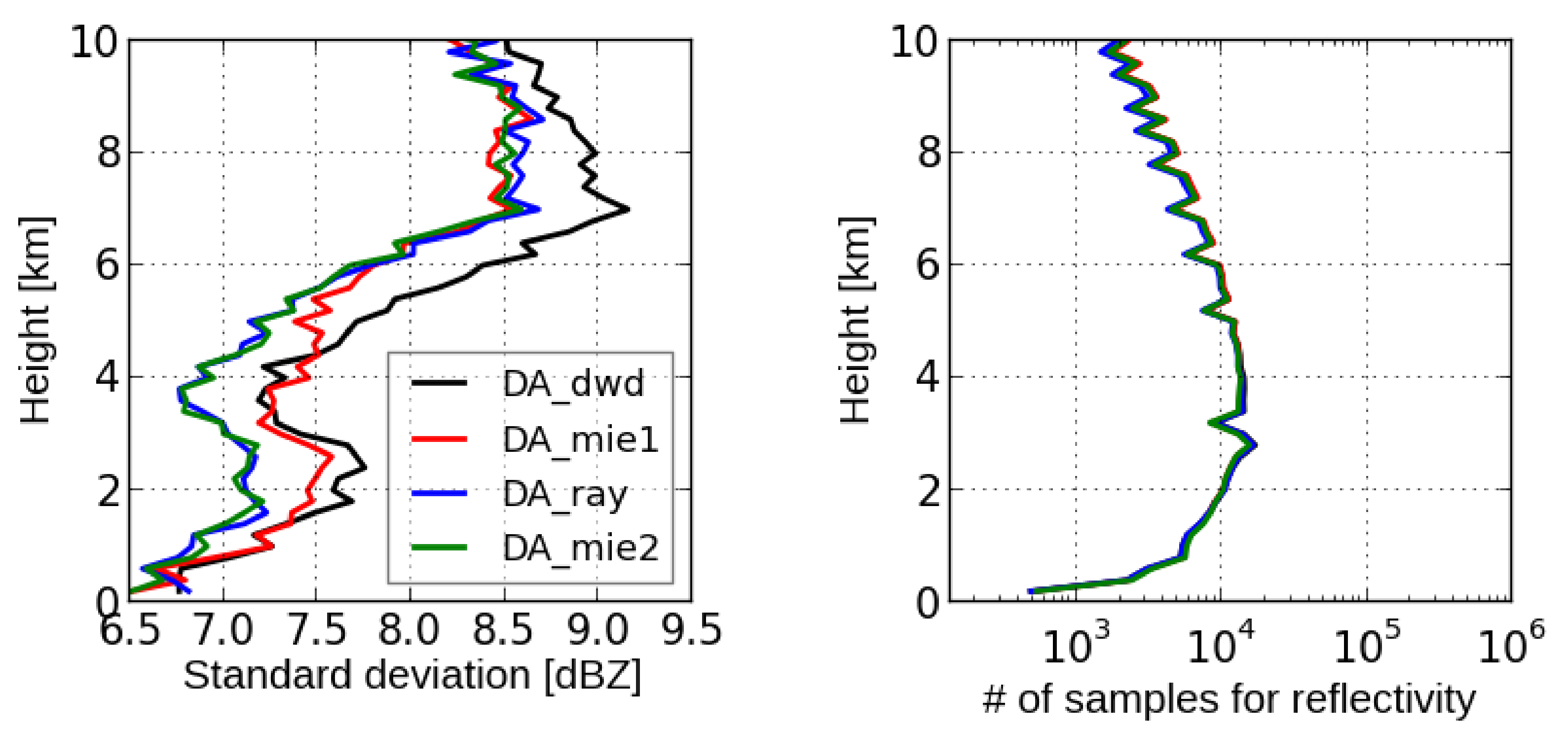
Figure 6 demonstrates vertical profiles of the estimated standard deviations of the OE for reflectivity data ≥ 5 dBZ at elevation 3.5° as well as numbers of samples used for estimation (varying between and , sufficient for robust statistics [33]). It is obvious that DA_dwd results in the largest standard deviations, mainly due to neglecting the beam broadening effect. Standard deviations of DA_mie1 are considerably smaller, especially at heights above 4 km. Compared to DA_mie1, DA_ray exhibits much smaller standard deviations between 2 and 6 km. As pointed out in Zeng et al. [5], this can be attributed to inappropriate microphysics melting parameterization in case of the Mie scattering scheme, and due to the vertical localization, the standard deviations around the melting layer are affected as well. By using the new parameterization, the standard deviations of DA_mie2 are very similar to those of DA_ray and even slightly smaller above 6 km.

Figure 6.
Vertical profiles of the estimated standard deviations of the OE for reflectivity data ≥ 5 dBZ at elevation 3.5° (left pannel) and the numbers of samples used for estimation (right panel). The samples are binned every 200 m in the vertical.
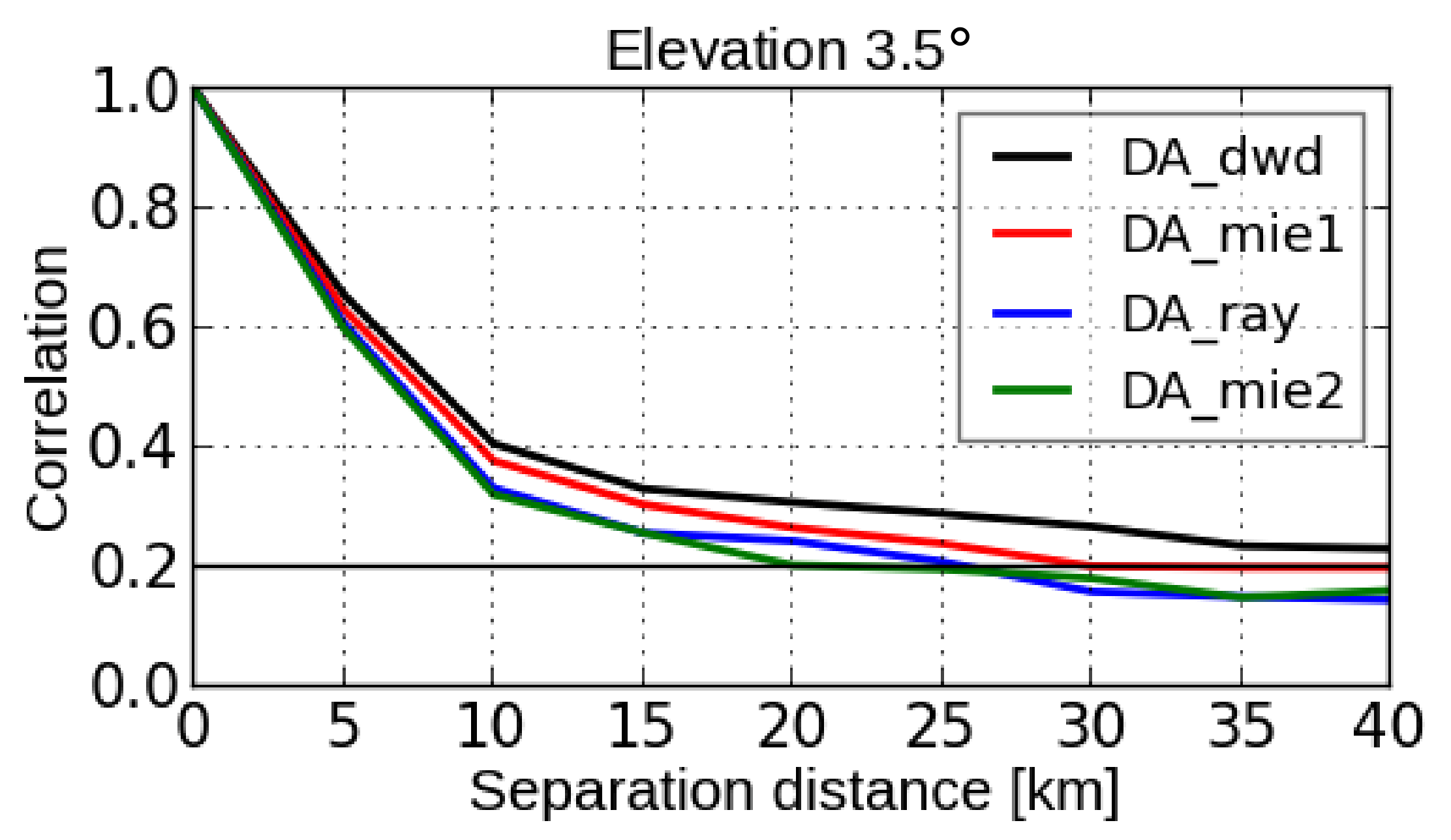
Figure 7 shows the horizontal correlations of the OE for reflectivity data ≥ 5 dBZ for elevation 3.5° at a height of 2.0 km. The horizontal correlation length scales of DA_dwd, DA_mie1, DA_ray, and DA_mie2 are about 40, 30, 25, and 20 km. As argued in Zeng et al. [5], the impacts of neglecting the beam broadening effect are neutral; therefore, the longest error correlation length scale of DA_dwd is due to the attenuation effect. By using the Rayleigh scheme in DA_ray, the length scale is shorter than in DA_mie1, and by using the new parameterization in case of the Mie scheme in DA_mie2, the shortest length scale is obtained.

Figure 7.
The estimated horizontal correlations of the OE for reflectivity data ≥ 5 dBZ for elevation 3.5° at heights of 2.0 km. For each elevation, the samples are binned every 5 km in the separation distance. As in Zeng et al. [5,26], Waller et al. [33], the correlation length scale is the distance where the correlation coefficient becomes not longer than 0.2.
5. Conclusions
The convective-scale data assimilation system ICON-D2-KENDA with the LETKF is operational at the DWD, and radar volume data are assimilated by using the forward operator EMVORADO, which is one of the most comprehensive operators at operational centers. In addition, LHN is employed to assimilate radar-derived precipitation rates. The goal of this work is to improve the LHN scheme as well as to reduce representation error of EMVORADO (denoted by “FE”) in the convective-scale data assimilation based on the ICON-D2-KENDA system for a summer period over Germany.
First of all, a series of one-month hindcasts are performed, in which two LHN schemes (LHN1 and LHN2) are compared with not using the LHN schemes. The scheme LHN1 generates temperature increments over the whole column and adapts accordingly so that the relative humidity remains unchanged. The LHN2 derives from increments of and are only available at points with occurrence of the saturation adjustment; therefore, the LHN2 is considered as an implicit approach to adjust T. It is shown by the CFADS of reflectivity that both LHN schemes produce closer frequency distributions to observed ones than no use of the LHN schemes, and the LHN2 scheme is better than the LHN1 scheme for reflectivities 10–30 dBZ between heights 4 and 7 km. Furthermore, it is shown by satellite-based pseudo-CFADS by using a visible channel to quantify cloud water/ice content and an infrared channel indicating cloud top height that both LHN schemes considerably improve the representation of middle clouds compared with no use of the LHN schemes but no clear differences results from two LHN schemes. In addition, hindcasts are also run to investigate the impacts of the beam broadening effect and the scattering schemes in EMVORADO. Compared to the CFADS of observed reflectivities, it is concluded that the beam broadening effect is more important at further distances and at the the melting layer and that the Mie scheme overestimates reflectivity values at the melting layer and the Rayleigh scheme as well as the Mie scheme with a new parameterization (to decrease the brightband effect) considerably reduce the overestimation. Secondly, a series of convective-scale data assimilation experiments in the ICON-D2-KENDA system are performed, based on different settings of EMVORADO, and the Desroziers method is used to estimate the statistics of the observation error (OE). In particular, it is found that the Mie scheme with the new parameterization for melting particles results in the smallest standard deviations of the OE and the shortest horizontal correlation length scale.
Overall, the current work uses the hindcasts to show the better performance of the LHN2, and it also demonstrates the importance of the beam broadening effect and the choice of the scattering schemes in EMVORADO, which are in line with the conclusion for the FE in Zeng et al. [5]. Moreover, the Mie scheme with the new parameterization for the melting particles proves to be the best in hindcasts as well as in estimation of the OE. A reduction in the FE and consequently in the OE will allow for better use of radar reflectivity observations in the data assimilation. Therefore, in the next steps, we will take advantage of the best settings of EMVORADO and its estimated statistics of the OE to improve the radar data assimilation in the ICON-D2-KENDA system, and the impacts on analyses and on forecast skills will be investigated.
Author Contributions
Conceptualization, Y.Z., Y.F., and A.d.L.; writing—original draft preparation, Y.Z.; analysis and writing—review and editing, all authors; supervision and project administration, Y.Z. and U.B. All authors have read and agreed to the published version of the manuscript.
Funding
This research was primarily supported by the Startup Foundation for Introducing Talent of NUIST. The work of U. Blahak and A. de Lozar is supported by the Innovation Programm for applied Research and Development (IAFE) of Deutscher Wetterdienst.
Data Availability Statement
Data used in this study are available upon request from the first author.
Acknowledgments
Thanks are given to Roland Potthast from the DWD and Yvonne Ruckstuhl from the LMU for technical supports.
Conflicts of Interest
The authors declare no conflict of interest.
References
- Schraff, C.; Reich, H.; Rhodin, A.; Schomburg, A.; Stephan, K.; Periáñez, A.; Potthast, R. Kilometre-Scale Ensemble Data Assimilation for the COSMO Model (KENDA). Q. J. R. Meteorol. Soc. 2016, 142, 1453–1472. [Google Scholar] [CrossRef]
- Hunt, B.R.; Kostelich, E.J.; Szunyogh, I. Efficient data assimilation for Spatiotemporal Chaos: A Local Ensemble Transform Kalman Filter. Phys. D Nonlinear Phenom. 2007, 230, 112–126. [Google Scholar] [CrossRef]
- Stephan, K.; Klink, S.; Schraff, C. Assimilation of radar-derived rain rates into convective-scale model COSMO-DE at DWD. Q. J. R. Meteorol. Soc. 2008, 134, 1315–1326. [Google Scholar] [CrossRef]
- Huo, Z.; Liu, Y.; Wei, M.; She, Y.; Fang, C.; Shu, Z.; Li, Y. Hydrometeor and Latent Heat Nudging for Radar Reflectivity Assimilation: Response to the Model States and Uncertainties. Remote Sens. 2021, 13, 3821. [Google Scholar] [CrossRef]
- Zeng, Y.; Li, H.; Feng, Y.; Blahak, U.; de Lozar, A.; Luo, J.; Min, J. Study on Sensitivity of Observation Error Statistics of Doppler Radars to the Radar forward Operator in convective-scale Data Assimilation. Remote Sens. 2022, 14, 3685. [Google Scholar] [CrossRef]
- Zeng, Y. Efficient Radar Forward Operator for Operational Data Assimilation within the COSMO-Model. Ph.D. Thesis, Karlsruhe Insititute of Technology, Karlsruhe, Germany, 2013. [Google Scholar]
- Zeng, Y.; Blahak, U.; Neuper, M.; Jerger, D. Radar Beam Tracing Methods Based on Atmospheric Refractive Index. J. Atmos. Ocean. Technol. 2014, 31, 2650–2670. [Google Scholar] [CrossRef]
- Zeng, Y.; Blahak, U.; Jerger, D. An efficient modular volume-scanning radar forward operator for NWP models: Description and coupling to the COSMO model. Q. J. R. Meteorol. Soc. 2016, 142, 3234–3256. [Google Scholar] [CrossRef]
- Blahak, U. RADAR_MIE_LM and RADAR_MIELIB—Calculation of Radar Reflectivity from Model Output. COSMO Technical Report No. 28, Consortium for Small Scale Modeling. 2016. Available online: http://www.cosmo-model.org/content/model/documentation/techReports/cosmo/docs/techReport28.pdf (accessed on 20 August 2022).
- Blahak, U.; de Lozar, A. EMVORADO—Efficient Modular Volume scan RADar Operator. A User’s Guide; Deutscher Wetterdienst: Offenbach, Germany, 2021. [Google Scholar]
- Geiss, S.; Scheck, L.; de Lozar, A.; Weissmann, M. Understanding the model representation of clouds based on visible and infrared satellite observations. Atmos. Chem. Phys. 2021, 21, 12273–12290. [Google Scholar] [CrossRef]
- Scheck, L.; Frerebeau, P.; Buras-Schnell, R.; Mayer, B. A fast radiative transfer method for the simulation of visible satellite imagery. J. Quant. Spectrosc. Radiat. Transf. 2016, 175, 54–67. [Google Scholar] [CrossRef]
- Scheck, L.; Weissmann, M.; Mayer, B. Efficient Methods to Account for Cloud-Top Inclination and Cloud Overlap in Synthetic Visible Satellite Images. J. Atmos. Ocean. Technol. 2018, 35, 665–685. [Google Scholar] [CrossRef]
- Desroziers, G.; Berre, L.; Chapnik, B.; Poli, P. Diagnosis of observation, background and analysis-error statistics in observation space. Q. J. R. Meteorol. Soc. 2005, 131, 3385–3396. [Google Scholar] [CrossRef]
- Lin, Y.; Farley, R.D.; Orville, H.D. Bulk parameterization of the snow field in a cloud model. J. Clim. Appl. Meteor. 1983, 22, 1065–1092. [Google Scholar] [CrossRef]
- Reinhardt, T.; Seifert, A. A three-category ice scheme for LMK. COSMO Newsl. 2006, 6, 115–120. [Google Scholar]
- Raschendorfer, M. The new turbulence parametrization of LM. COSMO Newsl. 2001, 1, 89–97. [Google Scholar]
- Tiedtke, M. A comprehensive mass flux scheme for cumulus parameterization in large-scale models. Mon. Weather Rev. 1989, 117, 1779–1799. [Google Scholar] [CrossRef]
- Oguchi, T. Electromagnetic wave propagation and scattering in rain and other hydrometeors. Proc. IEEE 1983, 71, 1029–1078. [Google Scholar] [CrossRef]
- Maxwell-Garnett, J.C. Colours in metal glasses and in metallic films. Proc. R. Soc. Lond. 1904, 203, 385–420. [Google Scholar]
- Bruggemann, D.A.G. Brechung verschiender physikalischer Konstanten von heteogenes Substanzen I. Dielektrizitätskonstanten und Leitfähigkeiten der Misachkörper aus isotropen Substanzen. Ann. Phys. 1935, 416, 636–664. [Google Scholar] [CrossRef]
- Saunders, R.; Hocking, J.; Rundle, D.; Rayer, P.; Havemann, S.; Matricardi, M.; Geer, A.; Lupu, C.; Brunel, P.; Vidot, J. RTTOV v12 Science and Validation Report. Technical Report. 2017. Available online: https://nwp-saf.eumetsat.int/site/download/documentation/rtm/docs_rttov12/rttov12_svr.pdf (accessed on 20 August 2022).
- Weston, P.P.; Bell, W.; Eyre, J.R. Accounting for correlated error in the assimilation of high-resolution sounder data. Q. J. R. Meteorol. Soc. 2014, 140, 2420–2429. [Google Scholar] [CrossRef]
- Lange, H.; Janjić, T. Assimilation of Mode-S EHS Aircraft Observations in COSMO-KENDA. Mon. Weather Rev. 2016, 144, 1697–1711. [Google Scholar] [CrossRef]
- Bormann, N.; Bonavita, M.; Dragani, R.; Eresmaa, R.; Matricardi, M.; McNally, A. Enhancing the impact of IASI observations through an updated observation-error covariance matrix. Q. J. R. Meteorol. Soc. 2016, 142, 1767–1780. [Google Scholar] [CrossRef]
- Zeng, Y.; Janjic, T.; Feng, Y.; Blahak, U.; de Lozar, A.; Bauernschubert, E.; Stephan, K.; Min, J. Interpreting estimated Observation Error Statistics of Weather Radar Measurements using the ICON-LAM-KENDA System. Atmos. Meas. Technol. 2021, 14, 5735–5756. [Google Scholar] [CrossRef]
- Yuter, S.E.; Houze, R.A. Three-dimensional kinematic and microphysical evolution of Florida cumulonimbus. Part II: Frequency distributions of vertical velocity, reflectivity, and differential reflectivity. Mon. Weather Rev. 1995, 123, 1941–1963. [Google Scholar] [CrossRef]
- Illingworth, A.J.; Hogan, R.J.; O’connor, E.J.; Bouniol, D.; Brooks, M.E.; Delanoe, J.; Donovan, D.; Eastment, J.; Gaussiat, N.; Goddard, J.; et al. Cloudnet: Continuous evaluation of cloud profiles in seven operational models using ground-based observations. Bull. Am. Meteorol. Soc. 2007, 88, 883–898. [Google Scholar] [CrossRef]
- Zhang, M.; Lin, W.; Klein, S.; Bacmeister, J.; Bony, S.; Cederwall, R.; Del Genio, A.; Hack, J.; Loeb, N.; Lohmann, U.; et al. Comparing clouds and their seasonal variations in 10 atmospheric general circulation models with satellite measurements. J. Geophys. Res. 2005, 110, D15S02. [Google Scholar] [CrossRef]
- Anderson, J.L. Spatially and temporally varing adaptive covariance inflation for ensemble filters. Tellus 2009, 61A, 72–83. [Google Scholar] [CrossRef]
- Zhang, F.; Snyder, C.; Sun, J. Impacts of initial estimate and observation availability on convective-scale data assimilation with an ensemble Kalman filter. Mon. Weather Rev. 2004, 132, 1238–1253. [Google Scholar] [CrossRef]
- Zeng, Y.; Janjić, T.; de Lozar, A.; Blahak, U.; Reich, H.; Keil, C.; Seifert, A. Representation of model error in convective-scale data assimilation: Additive noise, relaxation methods and combinations. J. Adv. Model. Earth Syst. 2018, 10, 2889–2911. [Google Scholar] [CrossRef]
- Waller, J.A.; Bauernschubert, E.; Dance, S.L.; Nichols, N.K.; Potthast, R.; Simonin, D. Observation Error Statistics for Doppler Radar Radial Wind Superobservations Assimilated into the DWD COSMO-KENDA System. Mon. Weather Rev. 2019, 147, 3351–3364. [Google Scholar] [CrossRef]
Publisher’s Note: MDPI stays neutral with regard to jurisdictional claims in published maps and institutional affiliations. |
© 2022 by the authors. Licensee MDPI, Basel, Switzerland. This article is an open access article distributed under the terms and conditions of the Creative Commons Attribution (CC BY) license (https://creativecommons.org/licenses/by/4.0/).

