1. Introduction
NASA’S Soil Moisture Active Passive (SMAP) mission was launched in January of 2015 with the goal of providing 9 km near surface soil moisture (NSSM) retrievals with high accuracy, global coverage, and a brief revisit time. With an effective sensing depth of ~0–5 cm, the SMAP L-band microwave radiometer produces high-sensitivity brightness temperatures (TBs) with spatial resolutions of ~40 km [
1]. By merging the ~40 km TBs with 3 km L-band radar data, SMAP retrieved 3 km and 9 km NSSM [
2]. Unfortunately, the SMAP radar transmitter malfunctioned in July of 2015, and only ~2.5 months of active-passive NSSM were retrieved. The SMAP team then created an alternative active-passive NSSM product, using Sentinel-1A/Sentinel-1B C-band Synthetic Aperture Radar (SAR) data. While this product has a spatial resolution of 1–3 km, full global coverage is only achieved every 12 days [
3].
NSSM measurements with both fine spatial scale and fine temporal scale are important for weather forecasting, hydrologic modeling, drought monitoring, and flood prediction [
4]. While a variety of remotely sensed NSSM products are available, they generally have either fine spatial resolution or fine temporal resolution, but not both. Microwave radiometers, like SMAP and Soil Moisture and Ocean Salinity (SMOS) [
5], retrieve NSSM at coarse spatial resolution (~40 km) and fine temporal resolution (~2–3 days). Microwave synthetic aperture radar (SAR), like Sentinel-1 [
6] and the upcoming NASA-ISRO SAR (NISAR) mission [
7], retrieve NSSM at fine spatial resolution (dozens of meters to 1 km) but coarse temporal resolution (~6–12 days). There is still a need for NSSM products with both fine spatial scale and fine temporal scale.
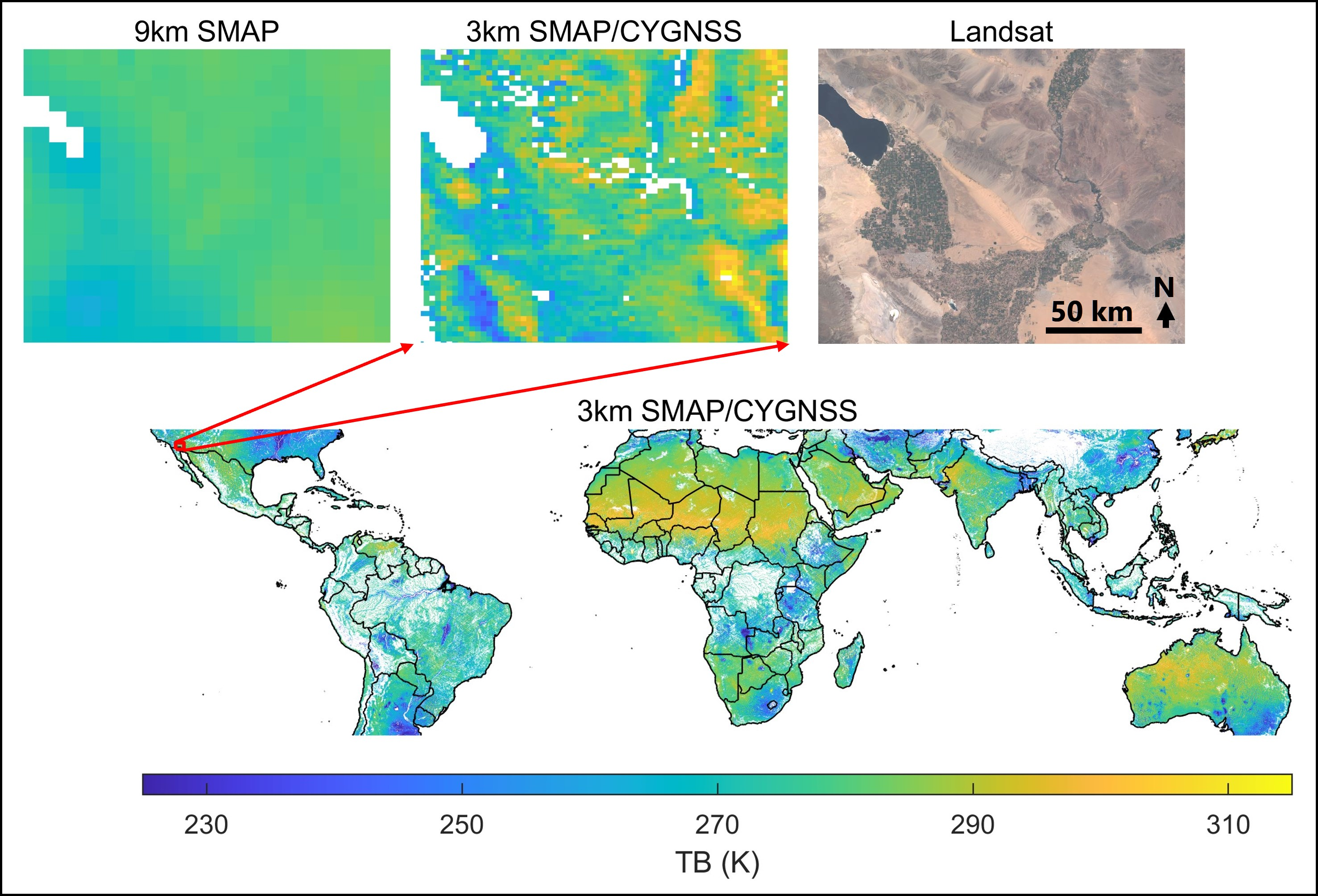
We developed an algorithm to downscale SMAP TBs using Cyclone Global Navigation Satellite System (CYGNSS) reflectivity data. The purpose of downscaling SMAP TBs is to represent the spatial heterogeneity of TB at a finer scale than possible via passive microwave data alone, with the end goal of developing a 3 km NSSM product. In this paper, we discuss the SMAP/CYGNSS TB downscaling algorithm, including the complexities involved in collocating SMAP and CYGNSS data. We also investigate the factors that affect the spatial variability of downscaled SMAP/CYGNSS TBs and analyze which types of landscapes produce the most and least spatially heterogeneous TBs. Finally, we discuss the primary sources of uncertainty associated with downscaled SMAP/CYGNSS TBs. Deriving NSSM from SMAP/CYGNSS TBs will be addressed in a separate paper.
Background
Each of the 8 CYGNSS observatories in orbit contains a bistatic radar receiver [
8]. Bistatic radar receivers collect radar signals sent from separate sources, in this case Global Positioning System (GPS) satellites, using a Signals-of-Opportunity retrieval method. CYGNSS retrievals therefore create a pseudo random spatial coverage pattern (
Figure 1), over a latitudinal range of ±38° [
8]. Like the SMAP radiometer, CYGNSS retrieves L-band microwave signals with a sensing depth of ~0–5 cm. Therefore, downscaling SMAP using CYGNSS provides an advantage over downscaling SMAP using Sentinel, as Sentinel retrieves C-band microwave signals with a sensing depth of ~0–2 cm [
1].
The spatial footprints of GNSS-R (Global Navigation Satellite System-Reflectometry) retrievals depend on the roughness of the surface. Most GNSS-R observations are a combination of coherent and incoherent reflections, with smooth, flat surfaces producing coherent reflections and rough, highly vegetated, or topographically variable surfaces producing incoherent reflections. For low-Earth orbit GNSS-R satellites, like CYGNSS, coherent reflections have a theoretical footprint of ~0.5 km and incoherent reflections have a theoretical footprint of ~25 km [
9]. While it is possible that future research will allow for the inclusion of a combination of incoherent and coherent scattering in our analysis of CYGNSS reflectivity data, for the time being we assume there is a strong coherent component in the reflectivity observations, and we correct the data accordingly. This assumption is based upon observational evidence of a significant degree of spatial heterogeneity at relatively small scales (~few km), even in the absence of inland surface water.
Assuming a coherently reflecting surface over land, the spatial footprint for a CYGNSS retrieval is ~0.5 × 7 km or ~0.5 × 3.5 km. The elongation is due to the time integration of the received signal. Before mid-2019, integration times were one second, which effectively smeared the along-track footprint to 7 km. After mid-2019, integration times were reduced to 0.5 s, which reduced the theoretical along-track footprint to 3.5 km [
10]. We chose to use a CYGNSS gridding scheme of 3 × 3 km, based on a study by [
11]. They found that R
2 and unbiased root mean square difference (ubRMSD) between SMAP and CYGNSS NSSM increased and decreased, respectively, as the CYGNSS NSSM gridding size decreased from 18 km to 9 km to 3 km. 3 km also falls within the SMAP EASE-Grid 2.0 gridding scheme [
1].
When CYGNSS data are gridded to 3 km (
Figure 1), the statistical repeat period is ~8–14 days, varying with latitude [
12]. The SMAP repeat period at low-to-mid latitudes is 2–3 days [
1]. If we choose a temporal collocation scheme that includes all CYGNSS observations (
Section 2.2.1), we can expect the average spatial coverage of 3 km CYGNSS observations within 9 km SMAP observations to range from ~14–38%. We calculated this by dividing the SMAP repeat period (2–3 days for full SMAP coverage) by the CYGNSS repeat period (8–14 days for full CYGNSS coverage). We further discuss SMAP/CYGNSS spatial coverage in
Section 4.5.
In the past several years, multiple NSSM algorithms have been developed using CYGNSS reflectivity data [
13,
14,
15,
16,
17]. However, similar to SAR NSSM data, CYGNSS and other GNSS-R NSSM data have lower accuracy than NSSM retrieved by radiometers, due to the larger surface roughness and vegetation effects of radar at smaller spatial scales [
18]. By merging SMAP and CYGNSS data, we aim to create a high accuracy NSSM product with a spatial scale of 3 km. To derive SMAP/CYGNSS NSSM, we first need to downscale SMAP TBs using CYGNSS reflectivity data.
2. Materials and Methods
To calculate downscaled SMAP/CYGNSS TB, we first calculated CYGNSS reflectivity. Next, we collocated SMAP and CYGNSS data, calculated the spatially-varying slopes of the linear regressions between SMAP emissivity and CYGNSS reflectivity, and used a variation of the SMAP active-passive TB downscaling algorithm to calculate 3 km SMAP/CYGNSS TB.
2.1. Calculating CYGNSS Reflectivity
CYGNSS Level 1 data are delay Doppler maps (DDMs), which map the power of the received signal with respect to time delay and Doppler shift [
8]. We derived CYGNSS reflectivity values using the peak power value of each DDM, from CYGNSS version 2.1 L1 data [
10]. We excluded all CYGNSS data with signal-to-noise ratios lower than 2 dB. This means the peak power values used to calculate reflectivity values were noticeably higher than the noise floors of the DDMs [
8].
The peak value of each CYGNSS DDM is the power received from the specular reflection point and must be corrected for antenna gain, the bistatic range, the GPS transmit power, and incidence angle, as described by [
14]. Assuming a coherent reflection, the coherent component of the bistatic radar equation can be used:
where
Pr is the uncorrected peak power of the DDM,
Pt is the transmitted power,
Gt is the transmitting antenna gain,
Gr is the receiving antenna gain,
λt is the transmitted GPS wavelength (0.19 m),
Rts is the distance from the transmitting antenna to the specular reflection point,
Rsr is the distance from the specular reflection point to the receiving antenna, and
Γs is the effective surface reflectivity.
We calculated
Γs by rearranging Equation (1) and converting all terms to dB:
Finally, we corrected for incidence angle using a modeled, theoretical formula of reflectivity with respect to incidence angle [
11,
15]. Assuming accurate knowledge of the terms in Equation (1), the final CYGNSS reflectivity (
) is only dependent on surface properties, including surface roughness, vegetation, and the dielectric constant, which depends on soil moisture.
2.2. Downscaling SMAP TB
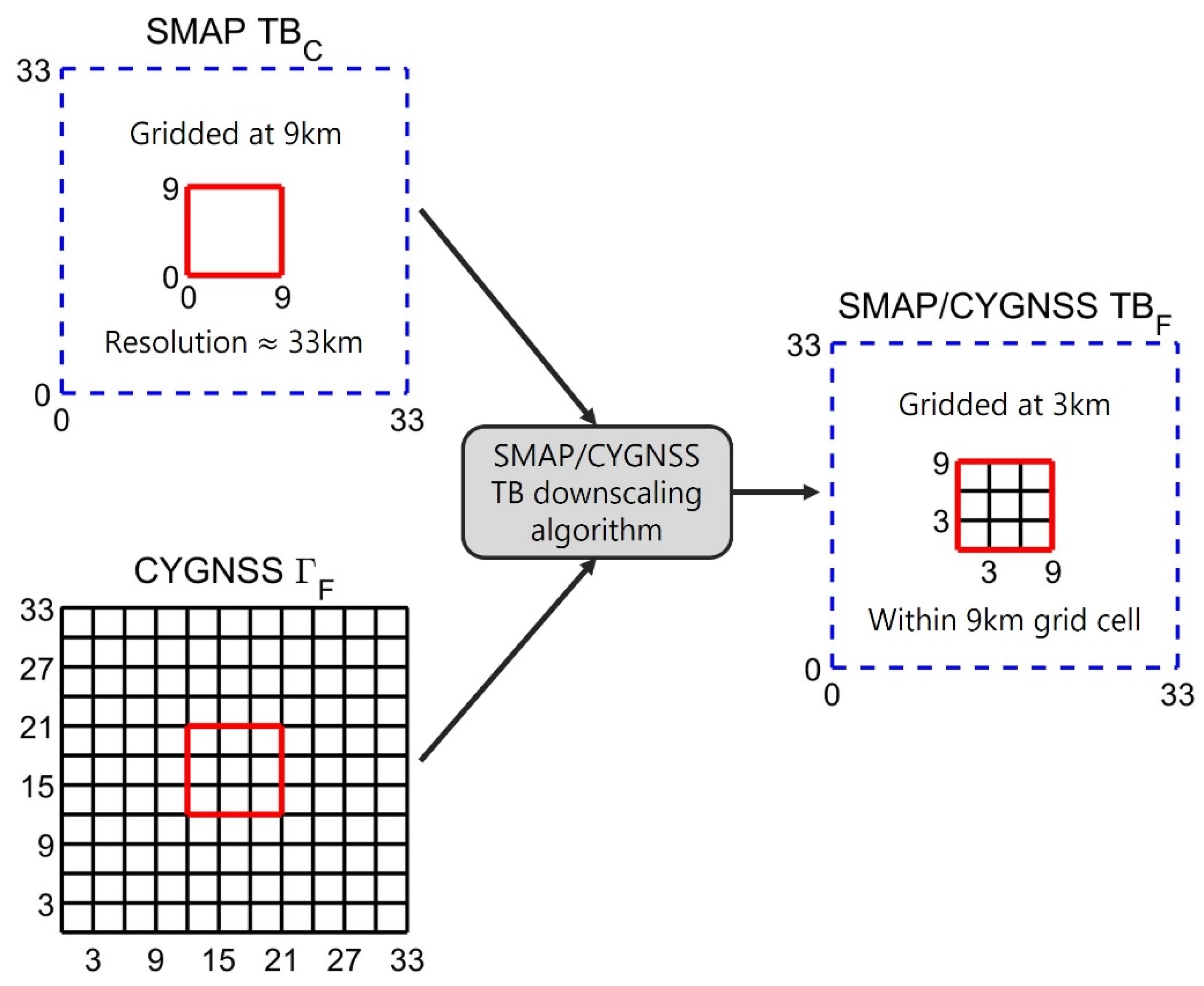
In an effort that follows the SMAP mission’s original plan to downscale radiometer TB retrievals using radar retrievals, we downscaled SMAP TBs using CYGNSS reflectivity values. SMAP’s original active-passive algorithm includes cross-polarization data, which is not available from CYGNSS retrievals. We therefore used a slightly modified version of the baseline SMAP active-passive TB algorithm (Equation (3)) with no cross-polarization measurements [
1]. This algorithm merges coarse-scale (33 km, gridded at 9 km) SMAP TBs with fine-scale (3 km) CYGNSS reflectivity values to create fine-scale (3 km) SMAP/CYGNSS TBs, as depicted in
Figure 2.
Here,
is the downscaled, SMAP/CYGNSS fine-scale brightness temperature, and
is the SMAP coarse-scale brightness temperature.
is fine-scale CYGNSS reflectivity and
is coarse-scale CYGNSS reflectivity.
and
are further discussed in
Section 2.2.3.
is the coarse-scale, spatially varying slope of the linear regression of SMAP emissivity and CYGNSS reflectivity values. Emissivity is defined as:
, where
is coarse-scale effective soil temperature, or surface temperature.
We used vertically polarized SMAP enhanced TBs, gridded at 9 km with a native resolution of approximately 33 km [
19], for our
values [
20]. We chose to use vertically polarized SMAP TBs because the SMAP NSSM algorithm using vertically polarized TBs outperforms the other NSSM algorithms [
19]. We used the GMAO GEOS-5 (Global Modeling and Assimilation Office, Goddard Earth Observing System version 5) effective soil temperature data provided with the SMAP enhanced product for our
values [
20]. An approximate equilibrium in temperature between the air, near-surface soil, and vegetation at 6am increases the accuracy of derived NSSM [
1]. We therefore only used 6am SMAP enhanced TBs (from descending orbits) in this study. We gridded 3 km
using the EASE-Grid 2.0.
The goal of downscaling SMAP TB is to represent the spatial heterogeneity of TB at a finer scale than possible using passive microwave data alone. 3 km SMAP/CYGNSS TB spatial heterogeneity is represented by spatial variations in
(Equation (3)) and is influenced by two factors. (1) Large spatial variations in CYGNSS reflectivity will create larger
ΔΓ values (
), which will increase the spatial variations of
. CYGNSS reflectivity varies due to natural spatial and temporal fluctuations in soil moisture, surface roughness, and vegetation. (2) More negative β values will also increase the spatial variations of
. SMAP/CYGNSS β values are further discussed in
Section 2.2.2.
Before we used Equation (3) to calculate , we first collocated SMAP TB and CYGNSS reflectivity data and calculated β.
2.2.1. Collocating SMAP TB and CYGNSS Reflectivity Data
We collocated SMAP TBs and CYGNSS reflectivity values in both space and time. We spatially collocated the fine-scale variables using the 3 × 3 km EASE-Grid 2.0. We spatially collocated the coarse-scale variables using 33 × 33 km boxes, centered on the 9 × 9 km EASE-Grid 2.0, as shown in
Figure 2. Each 33 km box consists of 11 × 11.3 km grid cells [
2,
3].
We masked out all 3 × 3 km grid cells containing semi-permanent open water. SMAP enhanced TB data are water body corrected, which result in higher TBs for adjusted grid cells [
21]. Consequently, matching SMAP and CYGNSS data over regions of open water will introduce error in the downscaled SMAP/CYGSS TBs. Using 30 m surface water data derived from Landsat [
22], available through the Global Surface Water Explorer, we calculated the percentage of each 3 × 3 km grid cell that contained open surface water for at least six months in 2018. We then implemented a water mask over regions that exceeded 5% semi-permanent open water.
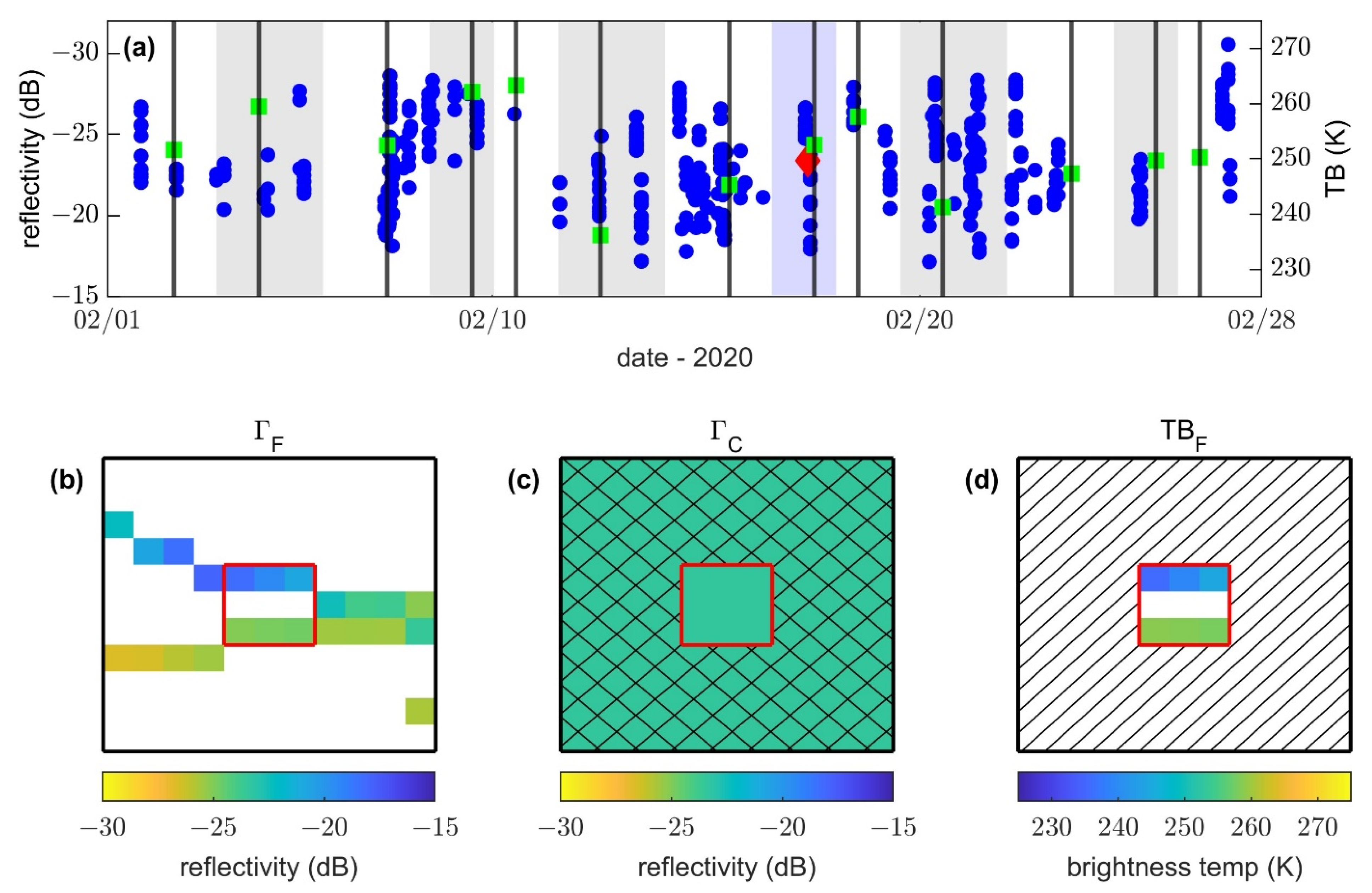
The temporal collocation scheme we used is ± half the time between successive SMAP observations. Since the time between SMAP observations is variable, the temporal collocation period varies from approximately 1–6 days. As can be seen in
Figure 3a, the “between-SMAP” temporal collocation scheme captures all CYGNSS data without reusing any CYGNSS data.
2.2.2. Calculating β
With more than five years of coinciding CYGNSS and SMAP data, there are sufficient collocated time-series data to calculate β statistically. As described above, β is the spatially varying slope determined via linear regression between SMAP emissivity and CYGNSS reflectivity values. We chose to use emissivity, rather than TB, because TB is affected by surface temperature, which fluctuates seasonally.
The β calculation is very important for the success and accuracy of the TB algorithm. β is essentially the scaling factor that adjusts
to be higher or lower than
, so an accurate representation of spatial variability depends on the estimated β value. Since the dielectric constant of soil varies based on water content, which affects the microwave emissivity of the soil [
23], SMAP emissivity decreases as NSSM increases and CYGNSS reflectivity increases as NSSM increases. Therefore, β values should theoretically be negative, and positive β values are unrealistic. Lower, or more negative, β values can produce larger differences between
and
, increasing spatial heterogeneity. As we show below, calculating β is challenging in some situations.
We experimented with a variety of options before determining an optimal β calculation method. Due to the ~8–14 day repeat period for CYGNSS at a 3 km scale [
12], the CYGNSS spatial coverage within a 33 km coarse-scale box on any given day is sparse. Therefore, daily CYGNSS observations within a 33 km box are not fully representative of its spatial heterogeneity. To account for this, we aggregated SMAP and CYGNSS data over 45-day periods. While longer periods provide slightly better correlation statistics, we chose this aggregation interval as a compromise to balance (1) the need for full CYGNSS coverage within 33 km boxes, (2) the need for ample data pairs for each linear regression, and (3) the ability to capture seasonal variations in soil moisture.
To calculate β, we located all CYGNSS reflectivity values within each 33 km box over 45-day periods and calculated the mean. Using the water mask described above, we excluded all CYGNSS observations within 3 × 3 km grid cells that exceeded 5% semi-permanent open water from our 45-day CYGNSS reflectivity means. We also calculated the mean of all SMAP emissivity values for each 33 km box over 45-day periods. Whereby, we calculated a single pair of SMAP and CYGNSS values for each 33 km box for each 45-day period. Using a calibration period of 1 April 2017 through 31 December 2020, this creates up to 29 data pairs for each linear regression.
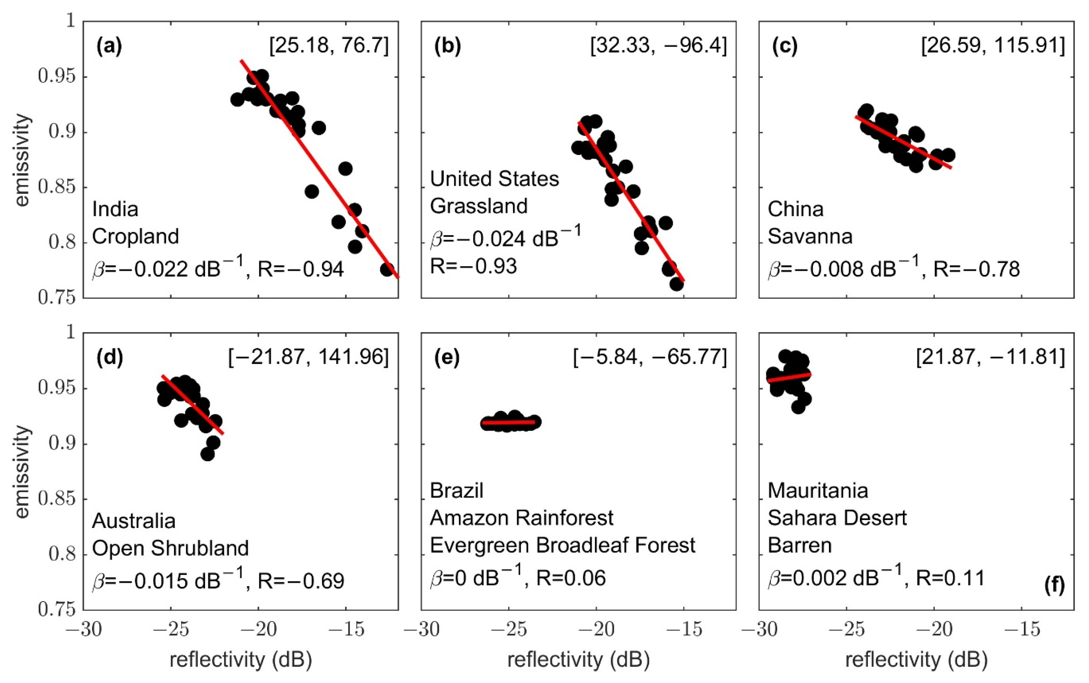
SMAP emissivity and CYGNSS reflectivity data pairs and their corresponding β values are vastly different from location to location (
Figure 4). In the results, we examine how these differences are affected by NSSM variability, mean annual precipitation, vegetation density, and topographic roughness.
2.2.3. Calculating
An illustration of the steps we used to calculate the 3 km SMAP/CYGNSS TBs (
) associated with a single 9 km SMAP enhanced TB (
) is provided in
Figure 3b. First, we calculated
by finding the median of all CYGNSS reflectivity values with specular points that fell within the appropriate 33 km box within ± half the time between successive SMAP observations. Second, we identified which of these CYGNSS reflectivity values had specular points that fell within the central 9 km grid cell and assigned these
to their appropriate 3 km grid cells. On the rare occasion that 2 or more CYGNSS observations fell within the same 3 km grid cell within ± half the time between successive SMAP observations, they were averaged. Finally, using Equation (3), we calculated
for each
. Regardless of whether
occurs on the same day as
, the output
are for the same day as
.
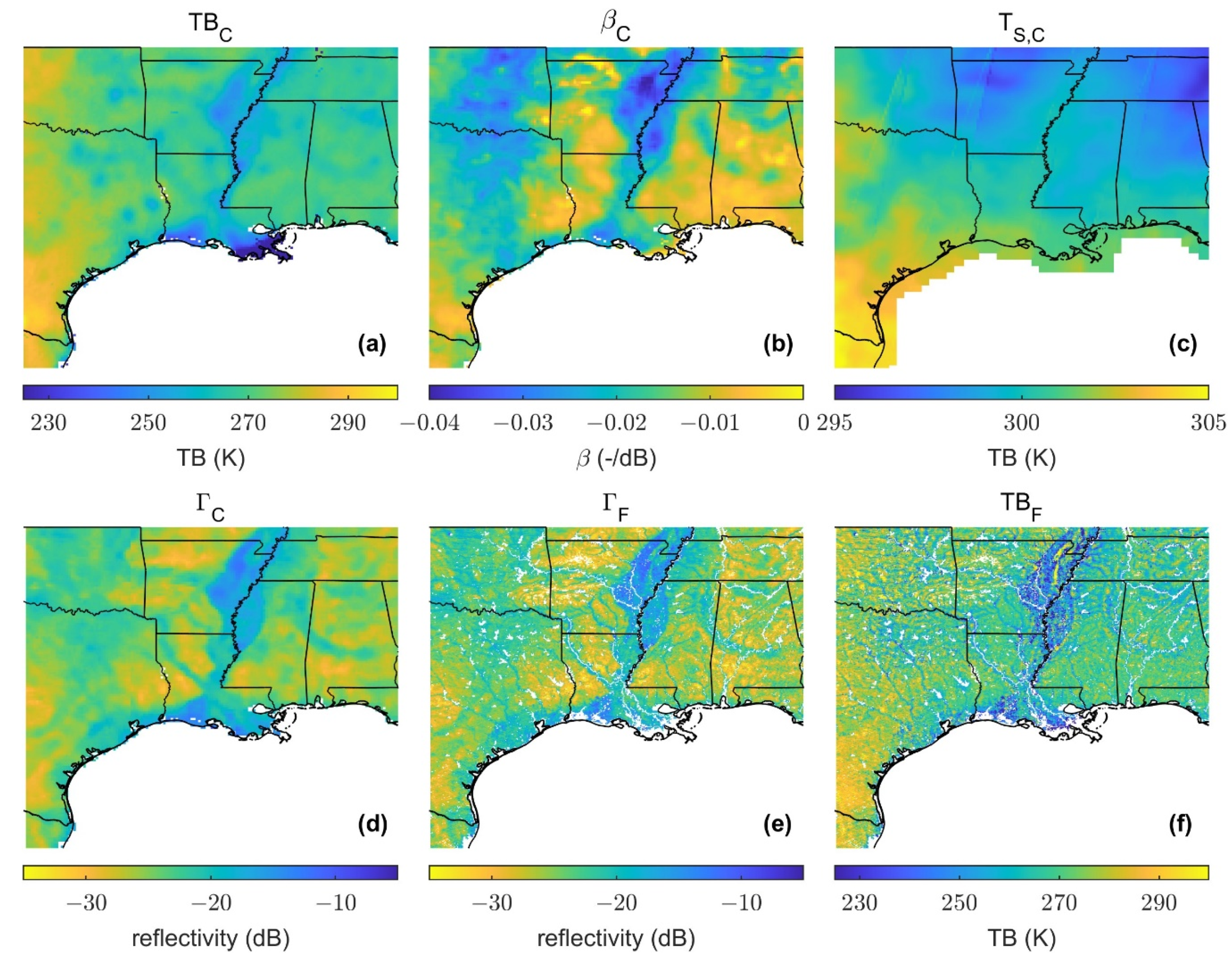
Figure 5 includes regional maps of all the parameters in the SMAP/CYGNSS TB algorithm (Equation (3)).
2.3. Auxiliary Data
To better understand the global spatial distribution of SMAP/CYGNSS β values, we compared β values with mean annual precipitation, mean NDVI, topographic roughness, and landcover class. We describe the data, processing, and upscaling methodology used to calculate each below.
We calculated global mean annual precipitation using monthly 0.1 × 0.1-degree CHIRPS (Climate Hazards Group InfraRed Precipitation with Station data) and RFE2 (National Oceanic and Atmospheric Administration Climate Prediction Center African Rainfall Estimation Algorithm v2) rainfall data from 2001–2020, archived by FLDAS (Famine Early Warning Systems Network Land Data Assimilation System) [
24]. We then upscaled the results to match our coarse-scale grid (33 km boxes, gridded at 9 km) using a linear averaging method.
We calculated mean NDVI using monthly 0.05 × 0.05-degree MODIS/Terra (Moderate Resolution Imaging Spectroradiometer) NDVI data from 2001–2020 [
25]. We then upscaled the results to match our coarse-scale grid (33 km boxes, gridded at 9 km) using a linear averaging method.
We calculated topographic roughness using the root-mean-square (RMS) surface height, derived from 90 m Shuttle Radar Topographic Mission (SRTM) digital elevation model (DEM) data [
26]. We calculated RMS surface height values to match our coarse-scale grid (33 km boxes, gridded at 9 km) using the following equation:
Here, is any given surface height value in the 33 km box, N is the total number of surface height values in the 33 km box, and is the mean value of surface heights within the 33 km box.
We used annual 0.05 × 0.05-degree MODIS IGBP (International Geosphere-Biosphere Programme) landcover class data [
27]. We upscaled the MODIS IGBP data to match our coarse-scale grids (33 km boxes, gridded at 9 km) using an areal-percent weighted average. For each 33 km box, we calculated the areal-percent of overlap for each 0.05 × 0.05-degree grid that overlapped or fell within the box. We multiplied the areal-percent weight by the percent-coverage of the dominant landcover class for the 0.05 × 0.05-degree grid and added it to a running sum for that landcover class. The largest landcover class running sum was assigned as the dominant landcover class of the 33 km box.
3. Results
Using the SMAP/CYGNSS TB downscaling algorithm (Equation (3)), TB spatial heterogeneity depends on the spatial variations in CYGNSS reflectivity (ΔΓ) and is scaled by β. We first present SMAP/CYGNSS TB spatial heterogeneity results, then we discuss the spatial patterns in ΔΓ values and β values. Finally, we present 3 km SMAP/CYGNSS TB results.
3.1. SMAP/CYGNSS TB Spatial Heterogeneity
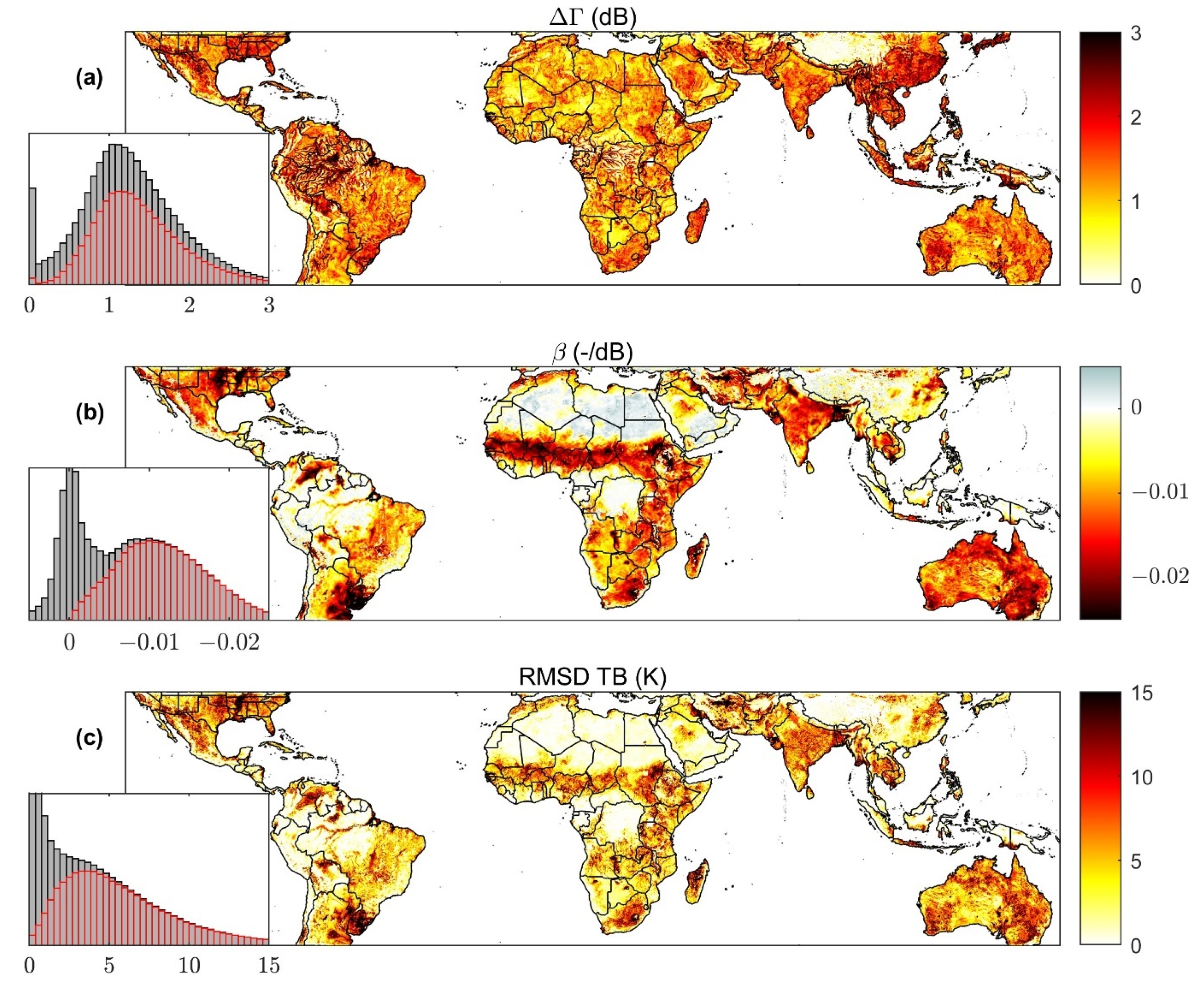
As expected, 3 km SMAP/CYGNSS TBs exhibit greater spatial variability than 9 km SMAP enhanced TBs. Comparing the 3 km SMAP/CYGNSS TBs associated with each 9 km SMAP TB allowed us to assess the spatial heterogeneity of 3 km SMAP/CYGNSS TBs. We calculated the RMSD between 9 km SMAP TBs and the corresponding 3 km SMAP/CYGNSS TBs for each SMAP observation with concurrent CYGNSS data during 2020. We then calculated the median RMSD TB for each 9 km grid cell. The median RMSD between 9 km SMAP TBs and 3 km SMAP/CYGNSS TBs range from 0.06 to 12.63 K (5th to 95th percentile) with a median of 3.03 K (
Figure 6c). Many of the near-zero RMSD TBs are due to likely-erroneous, near-zero β values (discussed below, in
Section 3.3). We can more accurately describe the spatial heterogeneity of 3 km SMAP/CYGNSS TBs by eliminating the near-zero RMSD TBs caused by near-zero β values. By only including β values with correlations less than −0.4, we exclude near-zero β values (
Figure 6b). We discuss the reasons for choosing a correlation cutoff of −0.4 in
Section 4.3. When only considering grid cells with β values with R < −0.4, the median annual RMSD between 9 km SMAP TBs and 3 km SMAP/CYGNSS TBs is 5.16 K (
Figure 6c).
3.2. Spatial Patterns in ΔΓ Values
Median ΔΓ values (
−
) range from 0.19 to 2.46 dB (5th to 95th percentile) with a median of 1.21 dB (
Figure 6a). We calculated the median magnitude of ΔΓ for each SMAP observation in 2020. Then, we calculated the median ΔΓ value for each 9 km grid cell.
The highest median ΔΓ values are found in north-central Mexico, southeast Asia, Japan, and western Australia. ΔΓ values are zero and near-zero in regions with high topographic roughness and in densely forested areas, due to low signal-to-noise ratios in the CYGNSS DDMs. The high median ΔΓ values seen over the Amazon and Central African rainforests are water signals, sometimes from beneath the canopy, and essentially map the regional tributaries [
28]. Looking closely at these densely forested regions, ΔΓ values are zero or near-zero everywhere besides the regional tributaries.
We expect ΔΓ values to be consistently low in dry and barren areas, due to limited changes in soil moisture and vegetation. However, median ΔΓ values fluctuate over the Sahara Desert. This might be due to sand dunes, rock outcrops, or other topographic and surface roughness variations throughout the desert.
The global spatial patterns in median ΔΓ (
Figure 6a) are not very similar to the spatial patterns in the median RMSD between 9 km SMAP TBs and 3 km SMAP/CYGNSS TBs (
Figure 6c). The correlation between median ΔΓ and median RMSD TB is 0.45. This suggests ΔΓ is not the primary source of SMAP/CYGNSS TB spatial heterogeneity, and instead β is the dominant factor.
3.3. Spatial Patterns in SMAP/CYGNSS β Values
SMAP/CYGNSS β values (the slopes of the linear regressions of SMAP emissivity and CYGNSS reflectivity) range from 0.002 to −0.021 dB
−1 (5th to 95th percentile) with a median of −0.007 dB
−1 (
Figure 6b). The global spatial patterns in β are similar to the spatial patterns in the median RMSD between 9 km SMAP TBs and 3 km SMAP/CYGNSS TBs (
Figure 6c). Regions with low β tend to have high RMSD TBs, and regions with near-zero β tend to have near-zero RMSD TBs. The correlation between β values and median RMSD TBs is −0.71. Therefore, β (not ΔΓ) is the primary source of SMAP/CYGNSS TB variations.
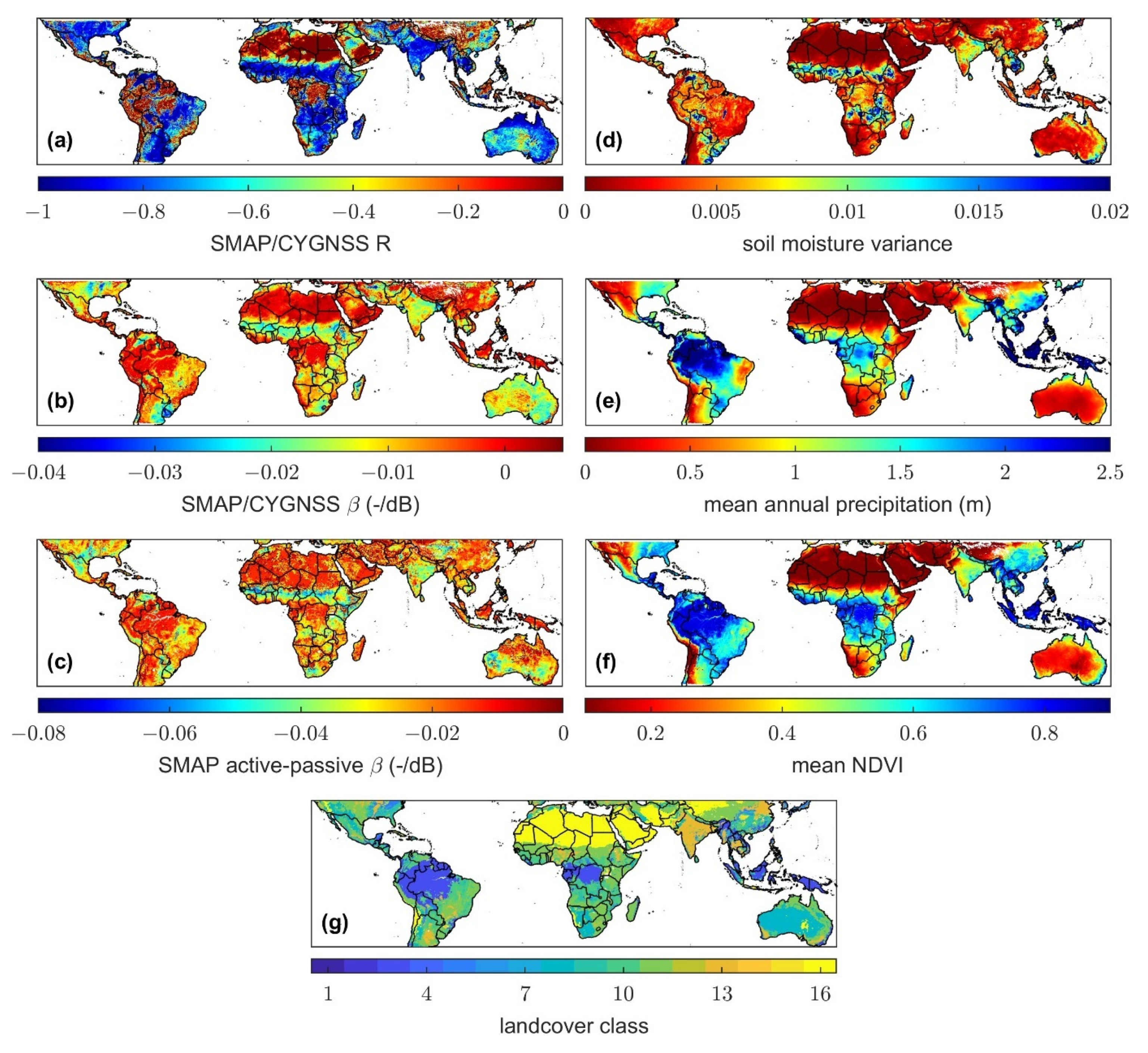
SMAP emissivity and CYGNSS reflectivity are strongly correlated in many areas (
Figure 7a). The median global correlation is −0.58, while the statistical mode of correlations is about −0.91. Linear regressions with near-zero correlations typically yield near-zero or positive β values (
Figure 7a,b). Given the SMAP/CYGNSS TB algorithm (Equation (3)), β values of zero necessitate that
will equal
. Therefore, near-zero β values yield low TB spatial heterogeneity. Additionally, as explained in
Section 2.2.2, positive β values are unrealistic. Near-zero and positive β values occur in dry areas (e.g., Sahara Desert), forested areas (e.g., Amazon Rainforest), and areas with high topographic roughness (e.g., Andes Mountains). We further investigate the factors that control the spatial patterns in β values below.
3.3.1. Relationships between Mean Annual Precipitation, NSSM Variability and β Values
SMAP emissivity and CYGNSS reflectivity are often poorly correlated in dry areas (
Figure 7a,d,e). This is because dry regions have little NSSM variability, and therefore little-to-no temporal variation in emissivity or reflectivity (
Figure 4f).
The impact of precipitation and NSSM variability on SMAP/CYGNSS β values can be illustrated by examining the seasonal cycle of β for a single 33 km box (
Figure 8). β is most negative (and correlation best) during the wet season, when NSSM is fluctuating due to rainfall events. In contrast, periods with no precipitation and low NSSM variability produce near-zero β values and poor correlations. We calculated seasonal β values using SMAP/CYGNSS data pairs that were temporally collocated using ± half the time between successive SMAP observations. The 45-day SMAP/CYGNSS β value (
Figure 8b), calculated using the methodology described in
Section 2.2.2, is closer to the seasonal β values generated during periods with higher precipitation and higher NSSM variability. This indicates that our 45-day β values provide an adequate estimate of the annual range of coarse-scale NSSM variability.
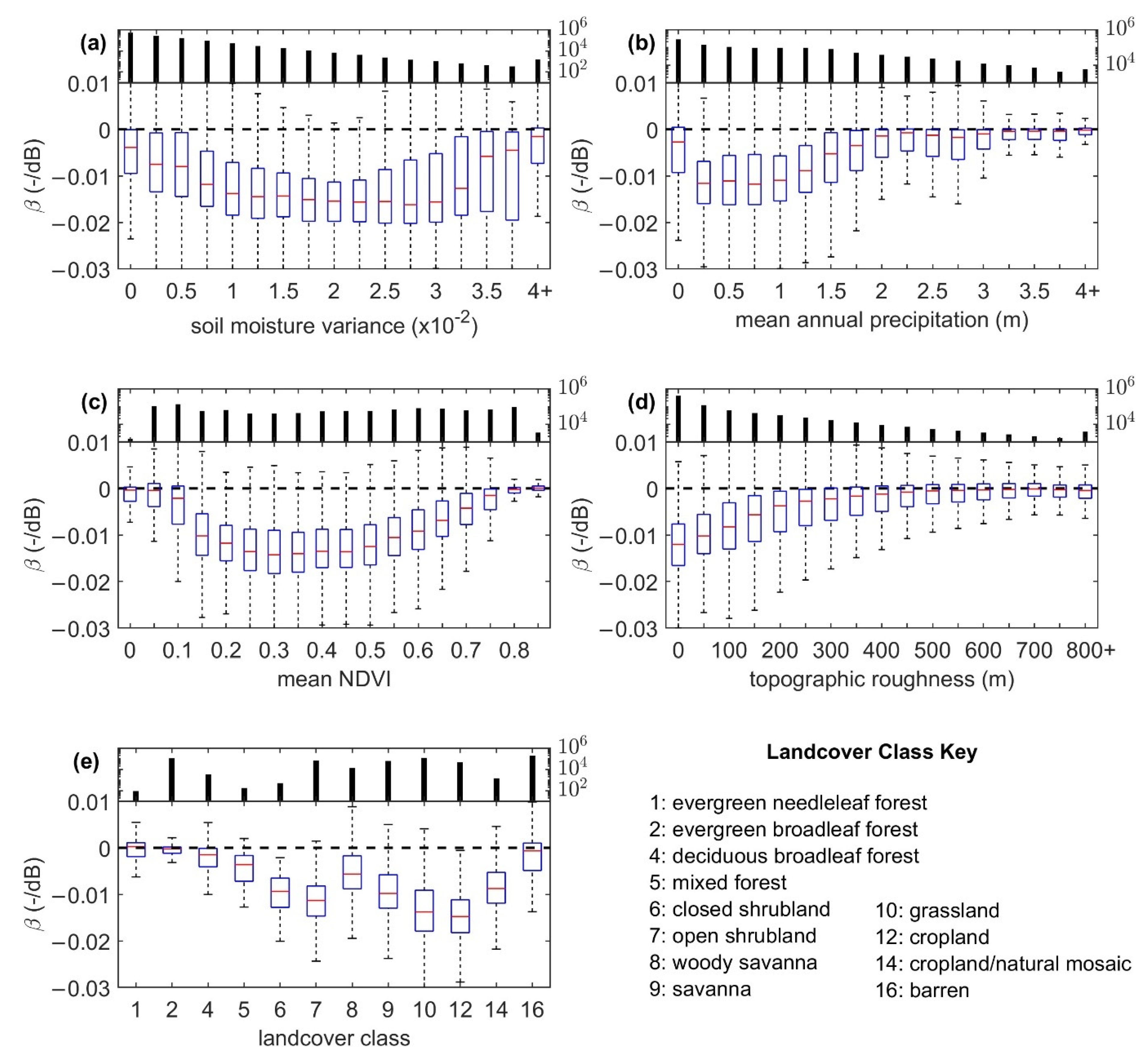
The relationship between SMAP/CYGNSS β values and NSSM variability is shown in
Figure 9a. We represented NSSM variability by calculating the variance through time of SMAP NSSM for each 9 km grid cell during 2020. The relationship between SMAP/CYGNSS β values and FLDAS mean annual precipitation (described in
Section 2.3) is shown in
Figure 9b. As expected, regions with very low NSSM variance (<0.0025) and very low mean annual precipitation (<0.25 m) have near-zero and positive β values. In contrast, the most negative β values are found in regions with moderate NSSM variance (~0.01–0.0325) and low-to-moderate mean annual precipitation (~0.25–1.5 m). The near-zero β values found in regions with high mean annual precipitation might be due to a lack of NSSM variability, if the soils are always wet, or could be due to increasing vegetation density, which is discussed below.
3.3.2. Relationship between NDVI and β Values
SMAP emissivity and CYGNSS reflectivity are often poorly correlated in forested areas (
Figure 6a,f) due to a lack of significant changes in both SMAP emissivity and CYGNSS reflectivity (
Figure 4e). This is because the dense vegetation in forests interferes with microwave sensing of the soil. We used MODIS/Terra mean NDVI (described in
Section 2.3) to compare SMAP/CYGNSS β values with vegetation density.
The relationship between SMAP/CYGNSS β values and mean NDVI is shown in
Figure 9c. As expected, areas with high mean NDVI values (>0.8) have near-zero SMAP/CYGNSS β values. Areas with low mean NDVI values (<0.1) also have near-zero SMAP/CYGNSS β values, because barren areas are usually very dry. In contrast, the most negative SMAP/CYGNSS β values, which ultimately lead to the greatest spatial heterogeneity in downscaled TBs, are found in areas with moderate mean NDVI values (~0.2–0.6).
3.3.3. Relationship between Topographic Roughness and β Values
SMAP emissivity and CYGNSS reflectivity are often poorly correlated in areas with high topographic roughness. Topographic roughness increases the uncertainty in both passive and active microwave remote sensing observations, due to increased scattering of the signal.
The positive relationship between SMAP/CYGNSS β values and SRTM topographic roughness (described in
Section 2.3) is shown in
Figure 9d, with β values approaching zero as topographic roughness increases. Since both dry and densely vegetated areas have near-zero β values, regardless of topographic roughness, we did not include any 9 km grid cells with mean annual precipitation less than 0.25 m or mean NDVI greater than 0.8 in our topographic roughness analysis.
3.3.4. Landcover Class and β Values
SMAP/CYGNSS β values also vary with MODIS IGBP landcover class (described in
Section 2.3), as shown in
Figure 9e. We only included β values in this analysis for 9 km grid cells that did not change landcover class during the period of our linear regression calculations (April 2017 through December 2020) and for 9 km grid cells that were greater than 90% the predominant landcover class by area. Since high topographic roughness produces poorly correlated SMAP/CYGNSS linear regressions and is not dependent on landcover class, we did not include any 9 km grid cells with topographic roughness values greater than 350 m in our landcover class analysis. Areas with topographic roughness greater than 350 m have β values of zero or higher more than 25% of the time (
Figure 9d). We did not include landcover classes that are masked out in NSSM products (0: water, 11: permanent wetland, 13: urban and built-up, and 15: snow and ice), nor did we include landcover classes without any 9 km grid cells meeting the criteria explained above (3: deciduous needleleaf forest).
β values are lowest in croplands (
Figure 4a) and grasslands (
Figure 4b) and highest in forests (
Figure 4e) and barren lands (
Figure 4f). Many of the landcover class and β value relationships can be explained by variations in NSSM variability, mean annual precipitation, and mean NDVI throughout landcover classes (
Figure 7d–g). We consider how to untangle these confounding effects in the discussion.
3.3.5. Comparison with SMAP Active-Passive β Values
Figure 6b,c compare SMAP/CYGNSS β values and SMAP active-passive β values. While some spatial disagreements exist, mainly in Australia, the United States, and the Middle East, general spatial agreement can be seen across most of the globe. Complete spatial agreement between β values is not expected, as NSSM variability affects β (
Section 3.3.1). Since there is no temporal overlap in SMAP active-passive data and CYGNSS data, and the calculation methods are not the same, a direct comparison of β values is not possible. The SMAP active-passive β values were calculated from 15 April–7 July 2015, and our SMAP/CYGNSS β values were calculated using data from April 2017–December 2020. The ~2.5 months of time-series data used to calculate SMAP active-passive β values is not representative of annual precipitation and NSSM variability, which may have caused incomplete β estimations, especially in arid regions [
2].
3.4. 3 km SMAP/CYGNSS TBs
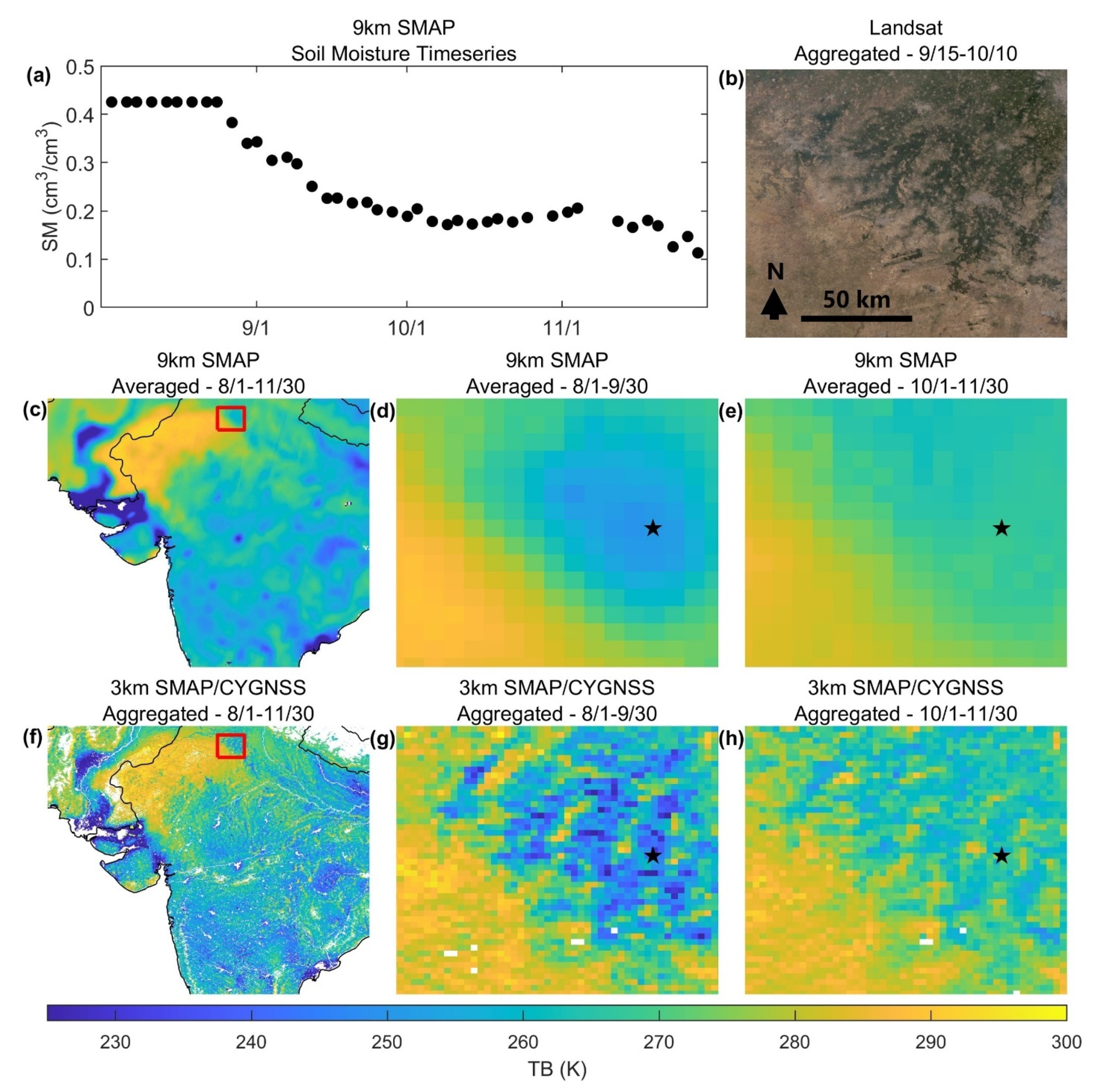
3 km SMAP/CYGNSS TBs include significantly more spatial detail than 9 km SMAP TBs and capture expected soil moisture patterns on the landscape. An example near New Delhi, India (
Figure 10) shows a decrease in soil moisture over croplands as time progresses from August to December. The drying of the croplands is evident in both 3 km SMAP/CYGNSS TBs (
Figure 10g,h) and 9 km SMAP TBs (
Figure 10d,e). However, the spatial pattern of the more productive croplands is obvious in 3 km SMAP/CYGNSS TBs but not discernible in 9 km SMAP TBs.
The 3 km SMAP/CYGNSS TB maps shown in
Figure 10g–h include data that is aggregated over 60 days. As such, adjacent 3 km TBs may be derived from SMAP/CYGNSS data observed on the same day, 5 days apart, or as many as 59 days apart. This introduces noise in the maps. We aggregated SMAP/CYGNSS TBs over 60 days due to sparse daily spatial coverage. Options for increasing daily spatial coverage in SMAP/CYGNSS TBs are discussed in
Section 4.5.
4. Discussion
4.1. Spatial Relationships Affecting β Values
We demonstrated the existence of spatial relationships between SMAP/CYGNSS β values and mean annual precipitation, NSSM variability, mean NDVI, and topographic roughness in
Section 3.3. However, which of these relationships are most important for determining β values? We synthesize the SMAP/CYGNSS β results below.
High topographic roughness decreases the correlation between emissivity and reflectivity, regardless of mean annual precipitation, NSSM variability, or mean NDVI. This does not mean that topographic roughness is a good indicator of β values, but rather that the quality of SMAP and CYGNSS observations is reduced in areas with high topographic roughness, due to increased scattering of the microwave signal.
While NSSM variability is related to mean annual precipitation, NSSM variability is more indicative of β values for two major reasons. First, both low and high mean annual precipitation can create areas with low NSSM variability. Second, NSSM variability can be affected by other factors, including seasonal flooding, irrigation, and the water and energy balance of the surface.
The two most important factors for determining β values are therefore NSSM variability and mean NDVI. β values generally decrease with increasing NSSM variability (
Section 3.3.1). Additionally, β values increase as mean NDVI increases from moderate-to-high values, due to increased vegetation density (
Section 3.3.2). NSSM variability is a better predictor of β values for areas with low-to-moderate mean NDVI, and mean NDVI is a better predictor of β values for areas with high mean NDVI.
The spatial relationships between SMAP/CYGNSS β values and mean annual precipitation, NSSM variability, and mean NDVI are also important when considering the β values produced by different landcover classes. Landcover classes with high mean NDVI (forests) and low mean annual precipitation and NSSM variability (barren areas) tend to produce poorly correlated linear regressions and near-zero β values. Alternatively, landcover classes with low-to-moderate mean annual precipitation, moderate NSSM variability, and moderate mean NDVI (shrublands, savannas, grasslands, and croplands) tend to produce well correlated linear regressions with more negative β values.
Similar findings are presented in [
30]. This study on the relationship between SMAP radar backscatter and SMAP radiometer TB found that linear correlations are best in grasslands and croplands and worst in forests and barren areas. They also found that linear correlations are best for moderate NDVI, with worse correlations for low and high NDVI, and that linear correlations improve as soil moisture variability increases.
4.2. Sources of Temporal Fluctuations in β Values
The temporal fluctuations in NSSM variability within 9 km grid cells significantly impact SMAP/CYGNSS β values (
Section 3.3.1).
Figure 8 demonstrates that β values vary significantly throughout the year, driven by seasonal changes in precipitation and NSSM variability. While seasonal changes in vegetation and surface roughness might also affect β values [
3], these signals would likely be dwarfed by seasonal changes in NSSM variability. Since SMAP/CYGNSS β values erroneously approach zero during the dry season, which could yield less spatial heterogeneity than exists, we chose not to use seasonally fluctuating β values. We therefore did not explore any possible temporal relationships between vegetation or surface roughness and β values.
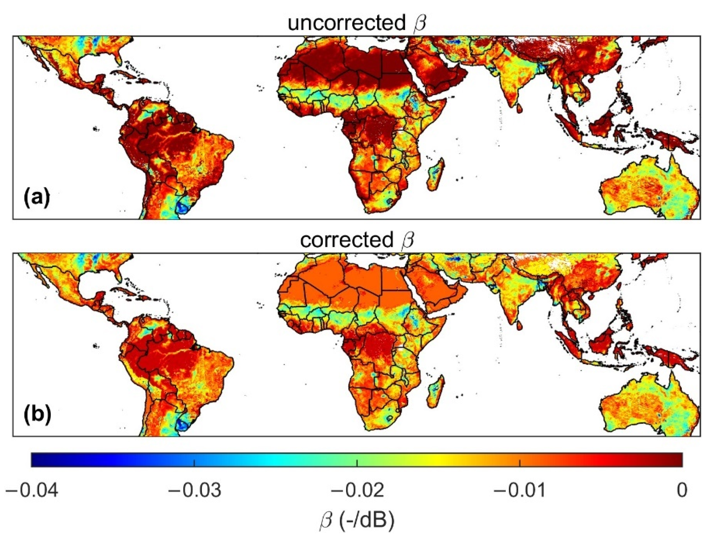
4.3. Correcting Problematic β Values
Near-zero SMAP/CYGNSS β values yield low TB spatial heterogeneity, and positive β values are unrealistic. Before calculating global SMAP/CYGNSS TB and NSSM, we plan to replace erroneous near-zero and positive SMAP/CYGNSS β values with realistic, representative β values. Since most near-zero and all positive β values have poor (near-zero or positive) correlations, we will implement a correlation cutoff to determine which β values to replace. We chose a preliminary correlation cutoff of −0.4, to ensure the replacement of erroneous β values while minimizing the number of replaced β values. Future work will include testing a variety of correlation cutoffs during NSSM validation.
Unlike the SMAP radar, CYGNSS does not include any cross-polarization data, so we are unable to replicate the regression model between cross-polarization backscatter (representative of vegetation level) and β used to create representative β values for the SMAP active-passive product [
2]. Instead, we will use the relationships between SMAP/CYGNSS β values and mean annual precipitation, mean NDVI, and NSSM variability to determine representative β values.
Since the variation in β values produced by different landcover classes can be explained by the relationships between β values and mean annual precipitation, mean NDVI, and NSSM variability (
Section 4.1), we will use landcover classes to create representative β values. Unfortunately, the correlation between β values and landcover class is not particularly high, as can be seen by the spread of the box and whisker plots in
Figure 9e. We therefore removed β values with correlations greater than −0.4 from the analyses. We calculated the median β value for each landcover class, including only 9 km grid cells with β values with R < −0.4. We then replaced β values where R > −0.4 with their median landcover class β values. Since MODIS landcover class changes annually, SMAP/CYGNSS β values will change annually.
Figure 11 shows a comparison of uncorrected and corrected β values.
4.4. TB Spatial Heterogeneity Comparisons
The goal of downscaling SMAP TB is to represent the spatial heterogeneity of TB at a finer scale than possible via passive microwave data alone. While we expect to see increased spatial heterogeneity at the 3 km scale compared to the 9 km or 33 km scale, the amount of additional heterogeneity depends on various landscape attributes. To gauge the accuracy of 3 km SMAP/CYGNSS TB spatial heterogeneity, we compare it to other TB datasets with similar spatial resolutions.
SMAP uses Passive Active L-band Sensor (PALS) flights during their calibration and validation campaigns. While no PALS flights are both spatially and temporally coincident with CYGNSS data, we can still use PALS data as a general comparison. During the SMAPVEX15 campaign in southeastern Arizona between 1 and 18 August 2015, the standard deviation of PALS 1 km TBs within 3 separate 36 km pixels during 7 overpasses varied from about 2–13 K [
31]. We calculated the standard deviation of 3 km SMAP/CYGNSS TBs within 33 km boxes covering approximately the same geographic area in Arizona between 1 and 31 August 2018 and found a range of about 0–16.9 K (5th–95th percentile). These TB standard deviations are fairly similar. We do not expect an exact match, as we are comparing two different scales (1 km vs. 3 km TBs) over 2 different years.
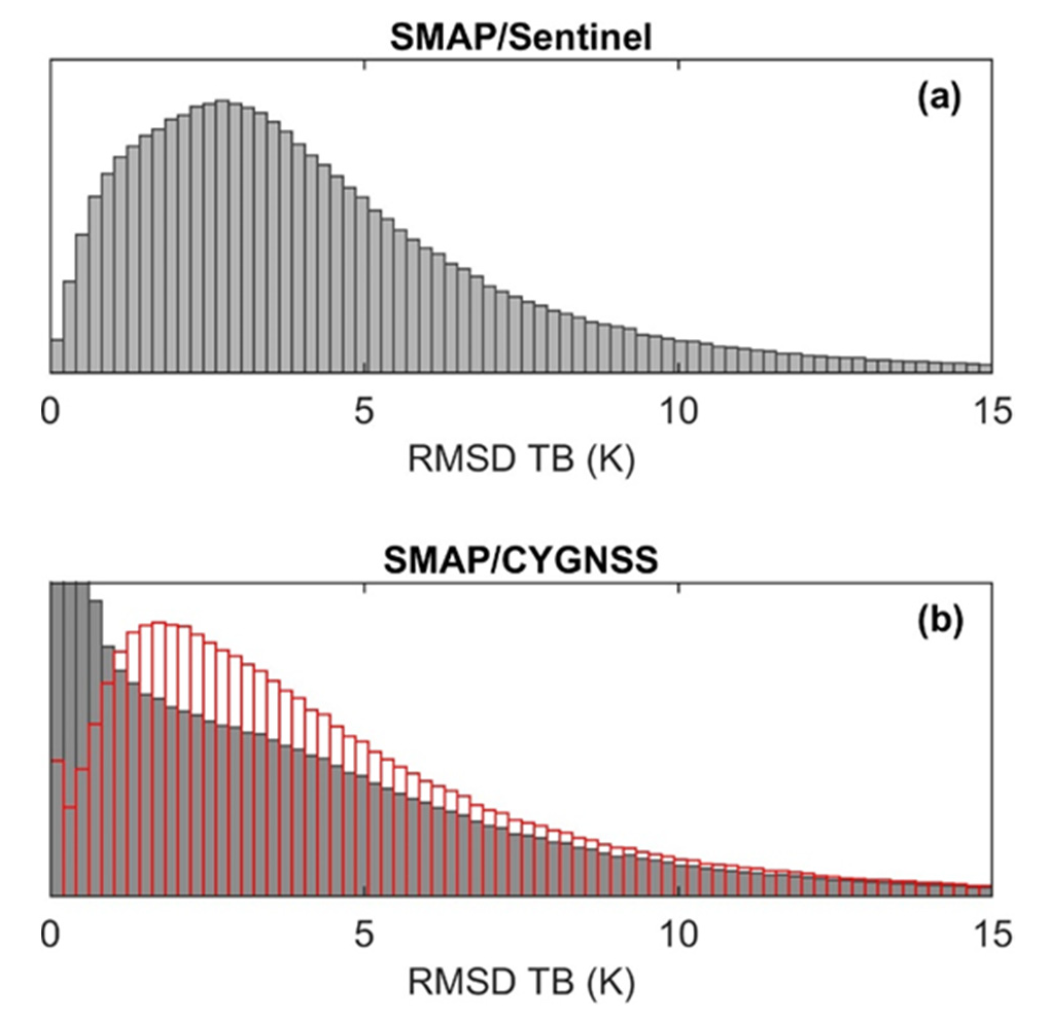
We also compared 3 km SMAP/CYGNSS TB spatial heterogeneity to 3 km SMAP/Sentinel TB spatial heterogeneity. Since CYGNSS retrieves L-band microwave signals and Sentinel retrieves C-band microwave signals, and CYGNSS and Sentinel observations are generally not concurrent, we do not expect an exact match. However, the spatial heterogeneity of different downscaled 3 km SMAP TBs should be similar.
We calculated the RMSD between 9 km SMAP TBs and the corresponding 3 km SMAP/CYGNSS or SMAP/Sentinel TBs [
32] for each SMAP observation with concurrent CYGNSS or Sentinel data between 1 April and 30 June 2018. We then calculated median RMSD TBs for each 9 km grid cell. We only included 9 km grid cells with both SMAP/CYGNSS and SMAP/Sentinel results in our analysis. The RMSD between 3 km SMAP/Sentinel TBs and 9 km SMAP TBs range from 0.8 to 11.7 K (5th–95th percentile) with a median of 3.7 K (
Figure 12a). The RMSD between 3 km SMAP/CYGNSS TBs and 9 km SMAP TBs range from 0.06 to 12.1 K (5th–95th percentile) with a median of 2.7 K (
Figure 12b). The lower median RMSD between SMAP/CYGNSS and SMAP TBs is primarily due to near-zero SMAP/CYGNSS β values. When we recalculate SMAP/CYGNSS TBs using landcover class corrected β values (
Section 4.3), the RMSD between 9 km SMAP TBs and 3 km SMAP/CYGNSS TBs range from 0.7 to 12.9 K (5th–95th percentile) with a median of 3.7 K (
Figure 12b). The similarity between SMAP/CYGNSS and SMAP/Sentinel 3 km TB spatial heterogeneity is promising.
4.5. SMAP/CYGNSS TB Spatial Coverage
SMAP/CYGNSS TBs do not provide full spatial coverage every 2–3 days, due to the ~8–14 day repeat period of CYGNSS observations at the 3 km scale. Low latitudes and areas where CYGNSS data have low signal-to-noise (i.e., forests and mountains) have worse spatial coverage. Higher latitudes and areas where CYGNSS data have high signal-to-noise (i.e., grasslands and croplands) have better spatial coverage.
The CYGNSS spatial coverage for each SMAP observation ranges from 3.0 to 28.3% (5th to 95th percentile) with a median of 15.5%. We calculated percent coverage for each 9 km SMAP TB during 2020 within ±35° latitude in non-mountainous and non-forested areas, using the associated 3 km SMAP/CYGNSS TBs. We then calculated the mean percent coverage for each 9 km grid cell.
There are two options for improving SMAP/CYGNSS TB spatial coverage. (1) We could produce both 3 km and 9 km SMAP/CYGNSS TBs. The 3 km TBs would include greater spatial heterogeneity, but the 9 km TBs would have better spatial coverage. Since the native resolution of SMAP enhanced TBs is ~33 km (gridded at 9 km), 9 km SMAP/CYGNSS TBs would still provide improved spatial heterogeneity. (2) We could use spatial interpolation techniques to fill the gaps. We could either (a) use pre-interpolated CYGNSS data, (b) interpolate 3 km SMAP/CYGNSS TBs, or (c) interpolate 3 km SMAP/CYGNSS NSSM. In each case, we could achieve full spatial coverage every 2–3 days, but precipitation patterns on the landscape would be less precise, which may lead to reduced NSSM accuracy. Future work will include analyzing the pros and cons of these options for improving SMAP/CYGNSS spatial coverage.
A final note: GNSS-R spatial coverage will likely improve in future years, due to larger constellation sizes and a higher number of received signals [
33,
34].
4.6. SMAP/CYGNSS TB Uncertainties
Multiple uncertainties exist related to the SMAP/CYGNSS TB algorithm. Some of these uncertainties are due to the difficulties of collocating SMAP and CYGNSS data, and others are inherent in CYGNSS data and the TB algorithm.
4.6.1. SMAP/CYGNSS Collocation Uncertainties
There are a few uncertainties related to the collocation of SMAP and CYGNSS data. First, since the temporal collocation period varies from 1–6 days, the chance of rainfall occurring between collocated SMAP and CYGNSS observations is non-negligible. Rainfall between collocated observations could lead to reduced accuracy in downscaled TBs, since the SMAP and CYGNSS observations being merged would not be representative of the same NSSM. Second, derived are not always representative of the spatial heterogeneity within a 33 km box. Due to the pseudo random spatial coverage of CYGNSS, some are calculated using a single CYGNSS reflectivity value, while other are calculated using tens of reflectivity values. When is calculated using a single reflectivity value, ΔΓ will always equal zero. Third, the moving window averaging method used to calculate , based on the coarse-scale gridding scheme, introduces bias into the downscaling algorithm. When the 3 km SMAP/CYGNSS TBs are upscaled, they do not always equal the 9 km SMAP TBs.
4.6.2. CYGNSS Reflectivity Uncertainties
Uncertainty in CYGNSS observations also introduces uncertainty into SMAP/CYGNSS TBs. CYGNSS data are calibrated to optimize retrievals over the ocean surface, which does not necessarily translate to an optimization of retrievals over land. In addition, there is uncertainty in some of the ancillary variables in the bistatic radar equation. Most prominently, the GPS effective isotropic radiated power (EIRP) for the v2.1 data is estimated from a lookup table and does not consider variations in transmit power over time or space. Some of the assumptions we made also introduce uncertainty into the reflectivity values: (1) the assumption that CYGNSS retrievals over land are based on completely coherent reflections; and (2) the 3 × 3 km gridding of CYGNSS reflectivity values, which does not account for the elongated footprint of CYGNSS observations. Future work will include estimating a bulk uncertainty for CYGNSS reflectivity values and propagating that uncertainty to TB and NSSM.
4.6.3. SMAP/CYGNSS TB Algorithm Uncertainties
Near-zero and positive β values, generally in areas with poorly correlated SMAP emissivity and CYGNSS reflectivity observations, are likely the greatest source of uncertainty in SMAP/CYGNSS TBs. While we will attempt to reduce some of this uncertainty by replacing poorly correlated β values with representative values (
Section 4.3), an incorrect β value has the potential to create significant uncertainty in calculated TBs. If we only consider β values with R < −0.4 (
Section 4.3 &
Figure 6b), the standard deviation of β values is 0.006 dB
−1. Using 5th to 95th percentile ranges in β, T
s, and ΔΓ, we determined that the potential RMSE in TBs based on β errors of ± 0.006 dB
−1 is ~3.5 K.
Other SMAP/CYGNSS TB sources of uncertainty include seasonal fluctuations in surface water not captured by our water mask, and uncertainty in surface temperature data. No water mask is perfect, and some TB uncertainty is expected near water bodies that fluctuate seasonally. Uncertainty related to surface temperature is primarily due to its coarse resolution. For consistency, we used the same surface temperature data as SMAP (GMAO GEOS-5), which has a native resolution of 0.25 × 0.3125-degrees. This coarse spatial resolution does not adequately capture the spatial heterogeneity of surface temperature on the landscape. Using a finer spatial resolution surface temperature would likely improve our downscaling algorithm and will be considered in the future.
5. Conclusions
We merged SMAP enhanced TBs and CYGNSS reflectivity values to create 3 km SMAP/CYGNSS TBs. Future work includes using 3 km SMAP/CYGNSS TBs to create a 3 km NSSM product.
Globally, the correlations between SMAP emissivity and CYNGSS reflectivity values are good (more negative), except in forested areas, barren areas, or areas with high topographic roughness. In this way, SMAP/CYGNSS β values are similar to SMAP active-passive β values [
2].
Lower β values yield greater spatial heterogeneity in SMAP/CYGNSS TBs. Areas with very low mean annual precipitation and NSSM variability have poorly correlated linear regressions with near-zero β values. Areas with high topographic roughness or high mean NDVI also have poorly correlated linear regressions with near-zero β values. Well correlated linear regressions with lower (more negative) β values are generally found in areas with low topographic roughness (<350 m), moderate NSSM variance (~0.01–0.0325), low-to-moderate mean annual precipitation (~0.25–1.5 m), and moderate mean NDVI (~0.2–0.6). β values are lowest in croplands and grasslands and highest in forested and barren lands.
3 km SMAP/CYGNSS TBs are more spatially heterogenous than 9 km SMAP TBs and capture expected soil moisture patterns on the landscape. The median RMSD between 3 km SMAP/CYGNSS TBs and 9 km SMAP TBs is 3.03 K. The spatial heterogeneity of 3 km SMAP/CYGNSS TBs is similar to the spatial heterogeneity of 3 km SMAP/Sentinel TBs.
In upcoming years, GNSS-R constellation sizes will increase, along with the number of received signals [
33,
34]. Additional GNSS-R constellations will provide more opportunities for downscaled NSSM products. Hopefully, the SMAP/CYGNSS TB algorithm can serve as a model for future downscaling efforts.
Author Contributions
Conceptualization, C.C.C. and E.E.S.; methodology, L.J.W., C.C.C., E.E.S. and N.N.D.; software, L.J.W. and C.C.C.; validation, L.J.W.; formal analysis, L.J.W.; resources, C.C.C. and E.E.S.; data curation, L.J.W. and C.C.C.; writing—original draft preparation, L.J.W.; writing—review and editing, E.E.S., C.C.C. and N.N.D.; visualization, L.J.W.; supervision, E.E.S. and C.C.C.; project administration, C.C.C. and E.E.S.; funding acquisition, C.C.C. and E.E.S. All authors have read and agreed to the published version of the manuscript.
Funding
This research was funded by the NASA Soil Moisture Active-Passive (SMAP) Science Team, award number 80NSSC20K1793.
Data Availability Statement
β values, their corresponding correlations, and median RMSD TB and ΔΓ values for 2020 (as shown in
Figure 6 and
Figure 7) are available in the
Supplementary Materials netcdf file. SMAP data is publicly available in the NSIDC DAAC [
20,
29,
32]. CYGNSS data is publicly available in the PO.DAAC [
10]. Downscaled SMAP/CYGNSS TB data will be publicly available with the downscaled SMAP/CYGNSS NSSM product in the future and are available on request from the corresponding author.
Acknowledgments
We would like to thank Andreas Colliander for helpful discussions regarding this project and Eric Smyth for help with batch processing and parallel computing. We would also like to thank anonymous reviewers for their constructive comments.
Conflicts of Interest
The authors declare no conflict of interest. The funders had no role in the design of the study; in the collection, analyses, or interpretation of data; in the writing of the manuscript; or in the decision to publish the results.
References
- Entekhabi, D.; Yueh, S.; O’Neill, P.E.; Kellogg, K.H.; Allen, A.; Bindlish, R.; Brown, M.; Chan, S.; Colliander, A.; Crow, W.T.; et al. SMAP Handbook: Soil Moisture Active Passive: Mapping Soil Moisture and Freeze/Thaw from Space; Jet Propulsion Laboratory, California Institute of Technology: Pasadena, CA, USA, 2014. Available online: https://smap.jpl.nasa.gov/system/internal_resources/details/original/178_SMAP_Handbook_FINAL_1_JULY_2014_Web.pdf (accessed on 30 October 2020).
- Das, N.N.; Entekhabi, D.; Dunbar, R.S.; Colliander, A.; Chen, F.; Crow, W.; Jackson, T.J.; Berg, A.; Bosch, D.D.; Caldwell, T.; et al. The SMAP Mission Combined Active-Passive Soil Moisture Product at 9 km and 3 km Spatial Resolutions. Remote Sens. Environ. 2018, 211, 204–217. [Google Scholar] [CrossRef]
- Das, N.N.; Entekhabi, D.; Dunbar, R.S.; Chaubell, M.J.; Colliander, A.; Yueh, S.; Jagdhuber, T.; Chen, F.; Crow, W.; O’Neill, P.E.; et al. The SMAP and Copernicus Sentinel 1A/B Microwave Active-Passive High Resolution Surface Soil Moisture Product. Remote Sens. Environ. 2019, 233, 111380. [Google Scholar] [CrossRef]
- Peng, J.; Albergel, C.; Balenzano, A.; Brocca, L.; Cartus, O.; Cosh, M.H.; Crow, W.T.; Dabrowska-Zielinska, K.; Dadson, S.; Davidson, M.W.J.; et al. A Roadmap for High-Resolution Satellite Soil Moisture Applications–Confronting Product Characteristics with User Requirements. Remote Sens. Environ. 2021, 252, 112162. [Google Scholar] [CrossRef]
- Kerr, Y.H.; Waldteufel, P.; Wigneron, J.; Delwart, S.; Cabot, F.; Boutin, J.; Escorihuela, M.J.; Font, J.; Reul, N.; Gruhier, C.; et al. The SMOS Mission: New Tool for Monitoring Key Elements of the Global Water Cycle. Proc. IEEE 2010, 98, 666–687. [Google Scholar] [CrossRef]
- Torres, R.; Snoeij, P.; Geudtner, D.; Bibby, D.; Davidson, M.; Attema, E.; Potin, P.; Rommen, B.; Floury, N.; Brown, M.; et al. Remote Sensing of Environment GMES Sentinel-1 Mission. Remote Sens. Environ. 2012, 120, 9–24. [Google Scholar] [CrossRef]
- Kellogg, K.; Rosen, P.; Barela, P.; Hoffman, P.; Edelstein, W.; Standley, S.; Dunn, C.; Guerrero, A.M.; Harinath, N.; Shaffer, S.; et al. NASA-ISRO synthetic aperture radar (NISAR) mission. In Proceedings of the 2020 IEEE Aerospace Conference, Big Sky, MT, USA, 7–14 March 2020; pp. 1–21. [Google Scholar]
- Ruf, C.; Chang, P.; Clarizia, M.P.; Gleason, S.; Jalenak, Z.; Majumdar, S.; Morris, M.; Murray, J.; Musko, S.; Posselt, D.; et al. CYGNSS Handbook: Cyclone Global Navigation Satellite System: Deriving Surface Wind Speeds in Tropical Cyclones; University of Michigan: Ann Arbor, MI, USA, 2016; Available online: https://cygnss.engin.umich.edu/wp-content/uploads/sites/534/2021/06/CYGNSS_Handbook_April2016.pdf (accessed on 27 September 2021).
- Katzberg, S.J.; Garrison, J.L. Utilizing GPS to Determine Ionospheric Delay over the Ocean. NASA Tech. Memo. 1996, 4750, 1–16. [Google Scholar]
- CYGNSS. CYGNSS Level 1 Science Data Record Version 2.1 [Data Set]. PO.DAAC, CA, USA. Available online: https://podaac.jpl.nasa.gov/dataset/CYGNSS_L1_V2.1 (accessed on 1 January 2022).
- Chew, C.; Small, E. UCAR/CU CYGNSS Soil Moisture Product: User Guide; University Corporation for Atmospheric Research: Boulder, CO, USA, 2019; Available online: https://data.cosmic.ucar.edu/gnss-r/soilMoisture/cygnss/level3/ucar_cu_sm_handbook.pdf (accessed on 22 October 2021).
- Chew, C. Spatial Interpolation Based on Previously-Observed Behavior: A Framework for Interpolating Spaceborne GNSS-R Data from CYGNSS. J. Spat. Sci. 2021, 1–14. [Google Scholar] [CrossRef]
- Chew, C.C.; Small, E.E. Soil Moisture Sensing Using Spaceborne GNSS Reflections: Comparison of CYGNSS Reflectivity to SMAP Soil Moisture. Geophys. Res. Lett. 2018, 45, 4049–4057. [Google Scholar] [CrossRef]
- Chew, C.; Small, E. Description of the UCAR/CU Soil Moisture Product. Remote Sens. 2020, 12, 1558. [Google Scholar] [CrossRef]
- Al-Khaldi, M.M.; Johnson, J.T.; O’Brien, A.J.; Balenzano, A.; Mattia, F. Time-Series Retrieval of Soil Moisture Using CYGNSS. IEEE Trans. Geosci. Remote Sens. 2019, 57, 4322–4331. [Google Scholar] [CrossRef]
- Clarizia, M.P.; Pierdicca, N.; Costantini, F.; Floury, N. Analysis of Cygnss Data for Soil Moisture Retrieval. IEEE J. Sel. Top. Appl. Earth Obs. Remote Sens. 2019, 12, 2227–2235. [Google Scholar] [CrossRef]
- Eroglu, O.; Kurum, M.; Boyd, D.; Gurbuz, A.C. High Spatio-Temporal Resolution Cygnss Soil Moisture Estimates Using Artificial Neural Networks. Remote Sens. 2019, 11, 2272. [Google Scholar] [CrossRef]
- Edokossi, K.; Calabia, A.; Jin, S.; Molina, I. GNSS-Reflectometry and Remote Sensing of Soil Moisture: A Review of Measurement Techniques, Methods, and Applications. Remote Sens. 2020, 12, 614. [Google Scholar] [CrossRef]
- Chan, S.K.; Bindlish, R.; Neill, P.O.; Jackson, T.; Njoku, E.; Dunbar, S.; Chaubell, J.; Piepmeier, J.; Yueh, S.; Entekhabi, D.; et al. Development and Assessment of the SMAP Enhanced Passive Soil Moisture Product. Remote Sens. Environ. 2018, 204, 931–941. [Google Scholar] [CrossRef] [PubMed]
- O’Neill, P.E.; Chan, S.; Njoku, E.G.; Jackson, T.; Bindlish, R.; Chaubell, J.; Colliander, A. SMAP Enhanced L3 Radiometer Global and Polar Grid Daily 9 km EASE-Grid Soil Moisture, Version 5 [Data Set]; NASA National Snow and Ice Data Center Distributed Active Archive Center: Boulder, CO, USA, 2021; Available online: https://nsidc.org/data/spl3smp_e/versions/5 (accessed on 21 January 2022).
- O’Neill, P.E.; Bindlish, R.; Chan, S.; Chaubell, J.; Njoku, E.; Jackson, T. Soil Moisture Active Passive (SMAP) Algorithm Theoretical Basis Document: Level 2 & 3 Soil Moisture (Passive) Data Products; Jet Propulsion Laboratory, California Institute of Technology: Pasadena, CA, USA; 2014. Available online: https://smap.jpl.nasa.gov/system/internal_resources/details/original/484_L2_SM_P_ATBD_rev_D_Jun2018.pdf (accessed on 16 June 2021).
- Pekel, J.F.; Cottam, A.; Gorelick, N.; Belward, A.S. High-Resolution Mapping of Global Surface Water and Its Long-Term Changes. Nature 2016, 540, 418–422. [Google Scholar] [CrossRef] [PubMed]
- Njoku, E.G.; Entekhabi, D. Passive Microwave Remote Sensing of Soil Moisture. J. Hydrol. 1996, 184, 101–129. [Google Scholar] [CrossRef]
- McNally, A. NASA/GSFC/HSL (2018), FLDAS Noah Land Surface Model L4 Global Monthly 0.1 × 0.1 Degree (MERRA-2 and CHIRPS) [Data Set]; Goddard Earth Sciences Data and Information Services Center (GES DISC): Greenbelt, MD, USA, 2018. Available online: https://disc.gsfc.nasa.gov/datasets/FLDAS_NOAH01_C_GL_M_001/summary (accessed on 10 June 2022).
- Didan, K. MOD13C2 MODIS/Terra Vegetation Indices Monthly L3 Global 0.05Deg CMG V006 [Data Set]. NASA EOSDIS Land Processes DAAC. 2015. Available online: https://lpdaac.usgs.gov/products/mod13c2v006/ (accessed on 14 June 2022).
- Jarvis, A.; Reuter, H.I.; Nelson, A.; Guevara, E. Hole-Filled SRTM for the Globe Version 4 [Data Set]. CGIAR-CSI SRTM 90m Database. 2008. Available online: http:/srtm.csi.cgiar.org (accessed on 1 October 2021).
- Friedl, M.; Sulla-Menashe, D. MCD12C1 MODIS/Terra+Aqua Land Cover Type Yearly L3 Global 0.05Deg CMG V006 [Data Set]. NASA EOSDIS Land Processes DAAC. 2015. Available online: https://lpdaac.usgs.gov/products/mcd12c1v006/ (accessed on 15 March 2022).
- Ruf, C.S.; Chew, C.; Lang, T.; Morris, M.G.; Nave, K.; Ridley, A.; Balasubramaniam, R. A New Paradigm in Earth Environmental Monitoring with the CYGNSS Small Satellite Constellation. Sci. Rep. 2018, 8, 1–13. [Google Scholar] [CrossRef]
- Entekhabi, D.; Das, N.; Njoku, E.G.; Johnson, J.T.; Shi, J. SMAP L3 Radar/Radiometer Global Daily 9 km EASE-Grid Soil Moisture, Version 3 [Data Set]; NASA National Snow and Ice Data Center Distributed Active Archive Center: Boulder, CO, USA, 2016; Available online: https://nsidc.org/data/spl3smap/versions/3 (accessed on 19 May 2022).
- Zeng, J.; Shi, P.; Chen, K.; Ma, H.; Bi, H.; Cui, C. On the Relationship Between Radar Backscatter and Radiometer Brightness Temperature From SMAP. IEEE Trans. Geosci. Remote Sens. 2022, 60, 1–16. [Google Scholar] [CrossRef]
- Colliander, A.; Cosh, M.H.; Misra, S.; Jackson, T.J.; Crow, W.T.; Chan, S.; Bindlish, R.; Chae, C.; Holifield Collins, C.; Yueh, S.H. Validation and Scaling of Soil Moisture in a Semi-Arid Environment: SMAP Validation Experiment 2015 (SMAPVEX15). Remote Sens. Environ. 2017, 196, 101–112. [Google Scholar] [CrossRef]
- Das, N.; Entekhabi, D.; Dunbar, R.S.; Kim, S.; Yueh, S.; Colliander, A.; O’Neill, P.E.; Jackson, T.; Jagdhuber, T.; Chen, F.; et al. SMAP/Sentinel-1 L2 Radiometer/Radar 30-Second Scene 3 km EASE-Grid Soil Moisture, Version 3 [Data Set]; NASA National Snow and Ice Data Center Distributed Active Archive Center: Boulder, CO, USA, 2020; Available online: https://nsidc.org/data/spl2smap_s/versions/3 (accessed on 3 June 2022).
- Ruf, C.S.; Norris, R.B.; O’Brien, A. Next Generation Bi-Static Radar Receiver for Possible CYGNSS Follow-On Mission. In Proceedings of the 99th American Meteorological Society Annual Meeting, Phoenix, AZ, USA, 6–10 January 2019. [Google Scholar]
- Freeman, V.; Esterhuizen, S.; Jales, P.; Masters, D. Spire’s new GNSS-R soil moisture products collected from small and innovative Earth observing satellites. In Proceedings of the SPIE: Remote Sensing for Agriculture, Ecosystems, and Hydrology XXII, online only, 21–25 September 2020. [Google Scholar]
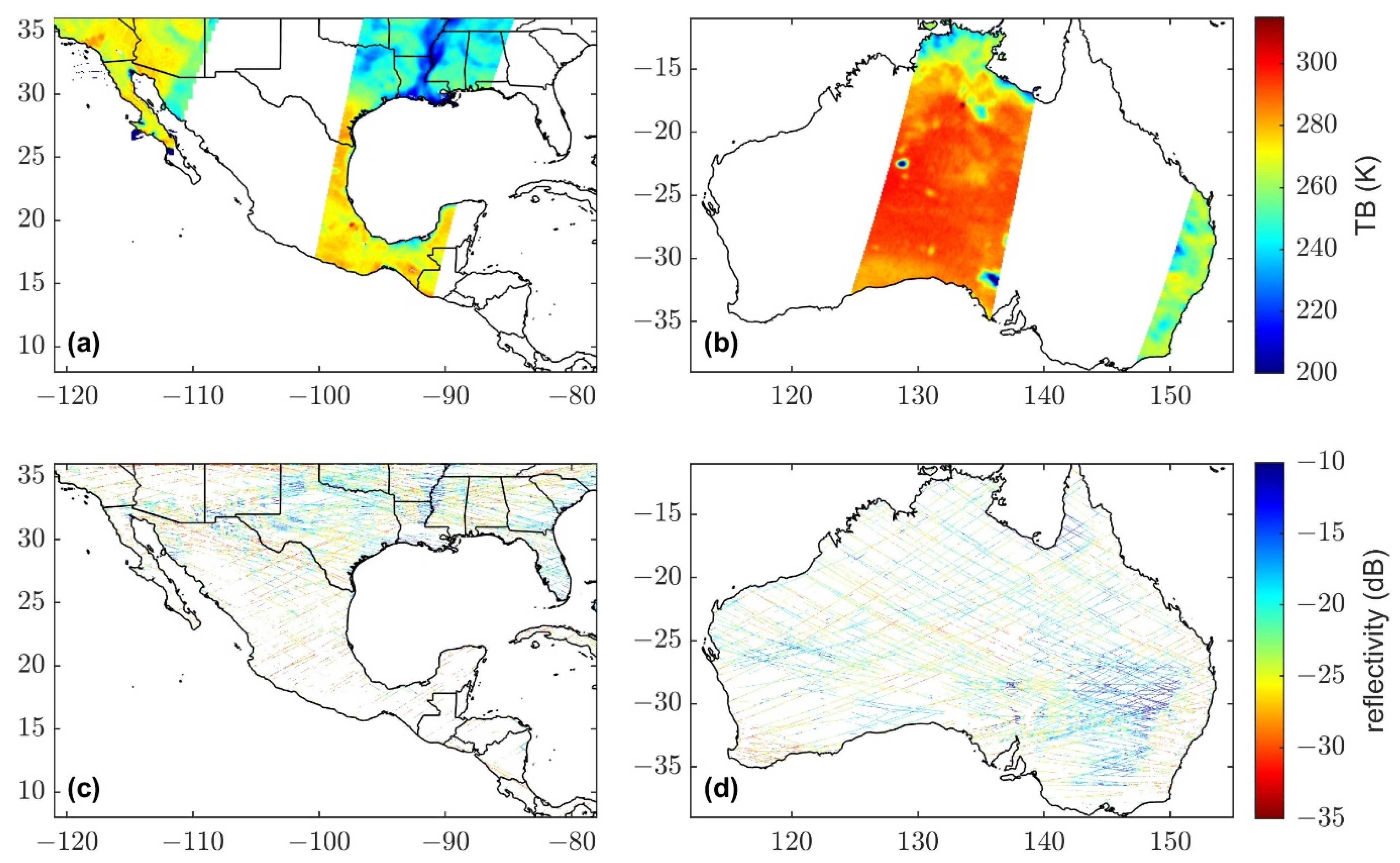
Figure 1.
9 km SMAP brightness temperatures (TBs) over (a) southern North America and (b) Australia, and CYGNSS reflectivity gridded at 3 × 3 km over (c) southern North America and (d) Australia on 9 March 2020.
Figure 1.
9 km SMAP brightness temperatures (TBs) over (a) southern North America and (b) Australia, and CYGNSS reflectivity gridded at 3 × 3 km over (c) southern North America and (d) Australia on 9 March 2020.
Figure 2.
We merged 9 km SMAP TBs with CYGNSS reflectivity data, gridded at 3 km, to create 3 km SMAP/CYGNSS TBs. 9 km SMAP TB data have a native resolution of approximately 33 km. To collocate SMAP and CYGNSS data, we derived 33 km boxes for each SMAP 9 km grid cell [
2,
3].
Figure 2.
We merged 9 km SMAP TBs with CYGNSS reflectivity data, gridded at 3 km, to create 3 km SMAP/CYGNSS TBs. 9 km SMAP TB data have a native resolution of approximately 33 km. To collocate SMAP and CYGNSS data, we derived 33 km boxes for each SMAP 9 km grid cell [
2,
3].
Figure 3.
All displayed data falls within the 33 km box centered on the 9 km grid cell at [31.2N, 98.7W]. In (b–d), the black borders are the 33 km box and the red squares are the 9 km grid cell. (a): A month-long timeseries of collocated SMAP and CYGNSS data, where each temporal collocation period is ±half the time between successive SMAP observations. The black lines denote the time of each SMAP observation, and the alternating gray and white shaded regions show the temporal collocation periods. The blue shaded region shows the collocation period depicted in (b–d). The green squares are SMAP observations. The blue dots are CYGNSS observations. The red diamond is the value shown in (c). (b): The map shows all the CYGNSS reflectivity values collocated with the SMAP observation on 17 February 2020. (c): is the median of all and is used to calculate within the central 9 km grid cell. (d) The map shows the 3 km SMAP/CYGNSS TBs calculated using the displayed and values.

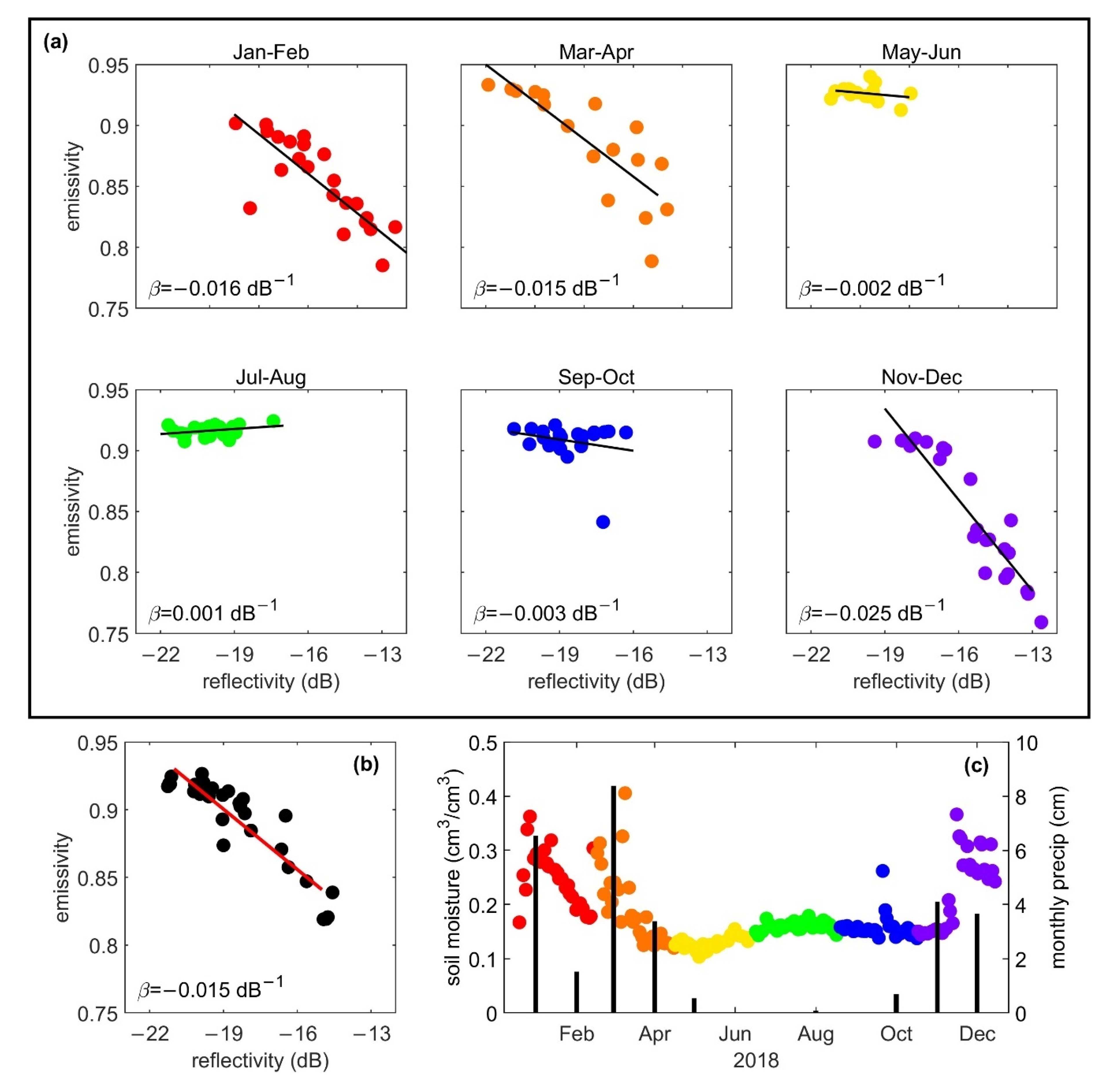
Figure 4.
Examples of 45-day SMAP emissivity and CYGNSS reflectivity data pairs and their corresponding linear regressions in (a) India, (b) the United States, (c) China, (d) Australia, (e) Brazil (Amazon Rainforest), and (f) Mauritania (Sahara Desert). Geographic coordinates, landcover class, β value (slope), and correlation value (R) are provided for each.
Figure 5.
Regional maps [25–37N, 85–99W] of all the parameters in the SMAP/CYGNSS TB algorithm. Each map is an aggregation of data from 1 June through 15 July 2020. (a) 33 km SMAP enhanced TB (gridded at 9 km), . (b) Slope of the linear regression between SMAP emissivity and CYGNSS reflectivity, . (c) Effective surface temperature, . (d) 33 km CYGNSS reflectivity (gridded at 9 km), . (e) 3 km CYGNSS reflectivity, . (f) 3 km SMAP/CYGNSS TB, .
Figure 6.
(
a) Map and histograms of median ΔΓ values (described in
Section 3.2), calculated using data from 2020. (
b) Map and histograms of SMAP/CYGNSS β values (described in
Section 2.2.2). (
c) Map and histograms of the median RMSD between 9 km SMAP TBs and 3 km SMAP/CYGNSS TBs (described in
Section 3.1), calculated using data from 2020. Gray histograms include all data. Red histograms only include data for 9 km grid cells with β values where R < −0.4 (
Section 4.3).
Figure 7.
(
a) Correlations for 45-day SMAP emissivity and CYGNSS reflectivity linear regressions (β values). (
b) SMAP/CYGNSS β values. (
c) SMAP active-passive β values. Mean of daily SMAP β (K/dB) divided by daily Ts (K) from 15 April 2015–7 July 2015 [
29]. (
d) NSSM variance, calculated using 9 KM SMAP soil moisture data from 2020. (
e) Mean annual precipitation, calculated using FLDAS precipitation data (described in
Section 2.3). (
f) Mean NDVI, calculated using MODIS/Terra data (described in
Section 2.3). (
g) 2020 MODIS IGBP landcover class. A landcover class key is included in the second figure in
Section 3.3.1.
Figure 8.
A depiction of the effect that NSSM variability has on β values. All displayed data falls within the 33 km box centered on the 9 km grid cell at [36.1N, 119.6W]. (
a) Bi-monthly SMAP emissivity and CYGNSS reflectivity data, collocated using ±half the time between successive SMAP observations, and their corresponding linear regressions. The seasonally varying β values are included in each plot. The SMAP/CYGNSS data points are colored to match the timeseries in (
c). (
b) 45-day SMAP emissivity and CYGNSS reflectivity data (as described in
Section 2.2.2) and the corresponding β value. (
c) SMAP NSSM timeseries with FLDAS monthly rainfall data. The NSSM data points are colored bi-monthly, to match the scatter plots in (
a).
Figure 9.
The number of 9 km grid cells (n-values) used to calculate each boxplot are included above each subplot. (a) Relationship between SMAP/CYGNSS β values and annual SMAP NSSM variance. Each boxplot spans a NSSM variance range of 0.0025. (b) Relationship between SMAP/CYGNSS β values and FLDAS mean annual precipitation. Each boxplot spans a precipitation range of 0.25 m. (c) Relationship between SMAP/CYGNSS β values and MOIDIS/Terra mean NDVI. Each boxplot spans an NDVI range of 0.05. (d) Relationship between SMAP/CYGNSS β values and SRTM topographic roughness. Each boxplot spans a topographic roughness range of 50 m. (e) Relationship between SMAP/CYGNSS β values and MOIDIS IGBP landcover class.
Figure 10.
A comparison of 9 km SMAP TBs and 3 km SMAP/CYGNSS TBs near New Delhi, India [28.25–29.5N, 75.5–77E]. (a) SMAP soil moisture timeseries for a single 9 km grid cell (location denoted by a black star in (d,e,g,h) from 1 August 2020 to 30 November 2020. (b) Landsat image aggregated from 15 September 2020 to 10 October 2020. This is the only relevant timeframe not obscured by clouds. (c) Regional [15–30N, 66–84E] 9 km SMAP TBs averaged from 1 August 2020 to 30 November 2020. The red box shows the area displayed in (d,e). (d) 9 km SMAP TBs averaged from 1 August 2020 to 30 September 2020. (e) 9 km SMAP TBs averaged from 1 October 2020 to 30 November 2020. (f) Regional [15–30N, 66–84E] 3 km SMAP/CYGNSS TBs aggregated from 1 August 2020 to 30 November 2020. The red box shows the area displayed in (g,h). (g) 3 km SMAP/CYGNSS TBs aggregated from 1 August 2020 to 30 September 2020. (h) 3 km SMAP/CYGNSS TBs aggregated from 1 October 2020 to 30 November 2020.
Figure 11.
(a) Uncorrected SMAP/CYGNSS β values. (b) Corrected SMAP/CYGNSS β values for 2020. All β values with R > −0.4 were replaced with representative β values, based on the median β values of the MODIS IGBP landcover classes.
Figure 11.
(a) Uncorrected SMAP/CYGNSS β values. (b) Corrected SMAP/CYGNSS β values for 2020. All β values with R > −0.4 were replaced with representative β values, based on the median β values of the MODIS IGBP landcover classes.
Figure 12.
(
a) RMSD between 3 km SMAP/Sentinel TBs and 9 km SMAP TBs. (
b) RMSD between 3 km SMAP/CYGNSS TBs and 9 km SMAP TBs. Gray histogram TBs were calculated using uncorrected β values. Red histogram TBs were calculated using landcover class corrected β values. The remaining zero-value RMSD TBs in the β-corrected histogram are due to ΔΓ values of zero, which occur when
is calculated using a single CYGNSS reflectivity value (
Section 4.6.1).
| Publisher’s Note: MDPI stays neutral with regard to jurisdictional claims in published maps and institutional affiliations. |
© 2022 by the authors. Licensee MDPI, Basel, Switzerland. This article is an open access article distributed under the terms and conditions of the Creative Commons Attribution (CC BY) license (https://creativecommons.org/licenses/by/4.0/).


