Abstract
Traditional synthetic aperture radar (SAR) autofocusing methods are based on the point-scattering model, which assumes the scattering phases of a target to be a constant. However, as for the distributed target, especially the arc-scattering target, the scattering phase changes with the observation angles, i.e., its scattering phase is time-varying. Hence, the compensated phases are a mixture of the time-varying scattering phases and the motion error phases in the traditional autofocusing methods, which causes the distributed target to be overfocused as a point target. To solve the problem, in this paper, we propose a SAR parametric autofocusing method with generative adversarial network (SPA-GAN), which establishes a parametric autofocusing framework to obtain the correct focused SAR image of the distributed targets. First, to analyze the reason for the overfocused phenomenon of the distributed target, the parametric motion error model of the fundamental distributed target, i.e., the arc-scattering target, is established. Then, through estimating the target parameters from the defocused SAR image, SPA-GAN can separate the time-varying scattering phases from the motion error phases with the proposed parametric motion error model. Finally, by adopting the traditional autofocusing method directly, SPA-GAN can obtain the correct focused image. Extensive simulations and practical experiments are carried out to demonstrate the effectiveness of the proposed method.
1. Introduction
A synthetic aperture radar (SAR) is a system that achieves two-dimensional high-resolution imaging by transmitting wideband signals and adopting synthetic aperture technology [1,2,3]. However, the motion error phases of the platform will cause the imaging result to be defocused and seriously affect the interpretation of the illuminated area [4]. To estimate and compensate for the motion error phases, many excellent SAR autofocusing methods have been proposed, which are mainly divided into the following two aspects.
The first type is based on image quality, e.g., minimum-entropy-based algorithm (MEA). The MEA estimates the motion error by minimizing the image entropy, and the motion error is usually modeled as a polynomial model to reduce the number of optimization variables [5,6,7]. However, it has high computational complexity and needs a lot of iterations to converge [8]. Moreover, it is difficult to set an appropriate learning rate. Too small or too large a learning rate will obtain a suboptimal solution. The second type is based on isolated strong points, e.g., phase gradient autofocus (PGA) algorithm: The PGA can quickly estimate and compensate for the motion error phases through the information of the echo signal itself and can handle the motion error phases of any order [9,10,11,12]. However, the performance of PGA heavily depends on the existence of the isolated strong points in the imaging scene.
In general, the traditional autofocusing methods (TAMs) are based on the point-scattering model, which consider that the phase modulation in the signal is the phase error caused by the motion error. Traditional airborne and spaceborne SARs have long observation distance and large swath. At this point, the illuminated scene contains abundant scattering information, which leads to fewer dominant scatterers. Therefore, robust autofocusing with TAMs can be achieved with multiple scattering units or all scattering units across the entire imaging swath.
However, in the cases of a distributed target whose scattering phases change drastically with observation angles and which lacks multiple relatively strong point-like targets, e.g., the vehicle-borne SAR imaging at short and medium range, ground-based radar imaging for an aerial cone-shaped target [13] and radar imaging for planet landforms [14], the phase modulation of the dominant distributed target may be caused by a combination of time-varying scattering and motion error. In these situations, the time-varying scattering phase is a normal phenomenon of fine-quality imaging and should not be classified as the phase error. At this point, if the TAMs are utilized to process the distributed target, there will be an overfocused phenomenon, i.e., the distributed target will be overfocused to a point target.
For the arc-scattering target (AST), the overfocused phenomenon occurs when TAM processes on an AST, i.e., the AST will be overfocused to a point-scattering target. As shown in Figure 1a–c, the metal top hat is overfocused to a point target after applying the TAM. Note that when the main lobe of the line-segment-scattering target is captured, the true contours of the line-segment-scattering target will be distorted by utilizing TAMs as well. Undoubtedly, this phenomenon brings the problem of target structure distortion when performing the autofocusing process in the aforementioned scenarios.
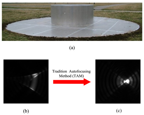
Figure 1.
Optical and SAR images of a metal top hat: (a) the optical image of the metal top hat; (b) the SAR image of the top hat under the influence of motion error; (c) the defocused SAR images after applying the TAM.
Hence, in this paper, we focus on solving the overfocusing problem of the AST, as shown in Figure 1c, since the arc-scattering target can represent both a point-scattering target and a line-segment-scattering target. From this perspective, theoretically, our proposed method is still adaptable to a certain extent when there is no interesting distributed target but only point-scattering targets in the scene.
To analyze the reason for the above overfocused phenomenon, first, it is necessary to analyze and model the overfocused phenomenon. Many researchers focus on characterizing the correlation between frequency and observation angles of some classic structures, and many scattering models are proposed, e.g., geometric theory of diffraction (GTD) model and the attributed scattering model (ASM) [15,16,17]. However, these models are not applicable under the influence of motion errors. The main reason is that the above models do not take into account the motion error, so they are unable to give a theoretical explanation for the overfocused phenomenon.
To solve the above problem, we must correctly estimate the phases caused by the real motion error. However, as we explained in Section 2.2, the motion error phases and the scattering phases will be coupled to each other under the influence of motion error; therefore, the parameters of the AST need to be estimated to decouple. Moreover, the phases after coupling are nonlinear because both the motion error phases and the angle-varying scattering phases are nonlinear. During the procedures of SAR autofocusing, the aforementioned TAMs adopt optimal image quality and linear unbiased minimum variance estimation to estimate the motion error phases [5,12]. However, for the above nonlinear coupling phase, the estimation methods adopted in the ATMs cannot correctly estimate the motion error due to the time-varying scattering phases.
Fortunately, in recent years, the emergence of deep learning (DL) technology makes it possible to solve the above nonlinear problem [18,19]. By using a multi-layered structure and embedding a nonlinear structure into the network layers, DL technology can solve many highly nonlinear problems in an extremely effective manner [20,21,22]. Generative adversarial network (GAN) is one of the most popular network architectures in the field of DL [23,24,25,26]. The main idea is to fit the mapping relationship between data distributions through the zero-sum game of the generator network and the discriminator network. GANs have been successfully applied to computer vision tasks, e.g., artificial image/video generation, image super-resolution, and text-to-image synthesis [27,28,29]. The applications of GANs in the SAR field mainly focus on the enhancement of SAR images, e.g., cloud removal, SAR image to optical image conversion, and SAR image denoising [30,31]. Guo used DCGANs to implement a SAR image simulator, which could be helpful to synthesize SAR images in a desired observation angle from a limited set of aspects [32]. Shi employed DCGAN for SAR image enhancement and used the result for the SAR-ATR task [33]. Zhang used DCGAN for transferring knowledge from unlabeled SAR images [34]. However, at this stage, the neural networks mainly focus on image vision and rarely involve parameter estimation [35]. So, they cannot directly solve the aforementioned overfocused problem.
In this paper, we propose an SAR parametric autofocusing method with generative adversarial network (SPA-GAN), which aims to make up for the deficiency of the point-scattering model when performing autofocusing processing for distributed targets. By introducing the scattering characteristics of the distributed target and establishing the framework of “parametric model → parameter estimation → SAR focusing”, this paper solves the problem of mismatch between traditional TAMs and an arc-scattering target. In particular, first, the arc-scattering parametric motion error model is established, which proves the AST will be overfocused to a point target with the ATMs. Then, the proposed SPA-GAN estimates the target parameters from the defocused image through the zero-sum game of the generator and discriminator, and the motion error phases and the arc-scattering phases are separated based on the proposed model.The proposed SPA-GAN in this paper is mainly applied for physical parameter estimation, where the estimated parameters can contribute additionally to the processing in SAR in [36,37,38]. Finally, since the arc-scattering phases have been separated, the motion error phases can be directly estimated and compensated for by adopting TAM to obtain a correct focused image.
The rest of this paper is organized as follows. In Section 2, we establish the arc-scattering parametric motion error model to analyze the overfocused phenomenon of the AST. In Section 3, the proposed SPA-GAN is developed to estimate the parameters of the AST and obtain the well-focused SAR image. In Section 4, simulation and real-data experiments are carried out to demonstrate the robustness of the proposed SPA-GAN and the effectiveness under different conditions. Finally, we discuss our finding, list our conclusions and outline our future work in Section 5 and Section 6.
2. Theoretical Analyses and Problem Formulation
In this section, we will introduce the overfocused phenomenon of the AST, and a parametric motion error model is proposed to explain the reason. Then, the problem formulation of the overfocused phenomenon will be analyzed in detail.
2.1. Phenomenon Presentation
According to the point-scattering model of the TAM [9], the motion error phases in Figure 2 can be expressed as:
where is the signal wavelength; is the azimuth time; are the point target coordinates; is the slant distance error; is the distance from the real radar platform to the point at ; is the distance from the ideal radar platform to the point at ; are the real trajectory position coordinates of the radar platform at ; are the ideal trajectory position coordinates of the radar platform at .
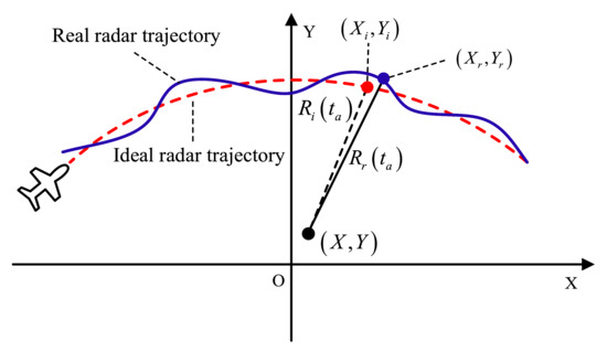
Figure 2.
Schematic diagram of the motion error geometric model of a point target.
According to the GTD [15], a distributed target with a curved edge appears as sliding scattering characteristics, i.e., the target appears as an AST in the SAR image. Therefore, we start from the most basic problem and simplify the distributed target with curved edges to the AST, as shown in Figure 3.
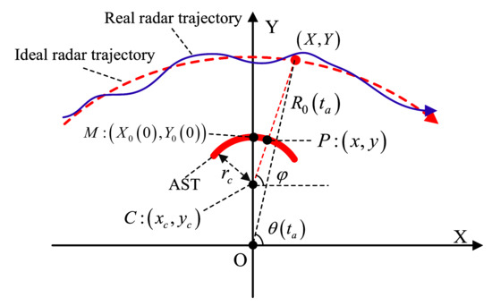
Figure 3.
Schematic diagram of the motion error geometric model of the AST.
After applying the TAM, we obtain the autofocusing result of the AST, as shown in Figure 4c. This result shows that when a TAM is utilized on the AST, the target will be overfocused to a point target. Undoubtedly, this kind of overfocused behavior will lead to the failure of image information interpretation.
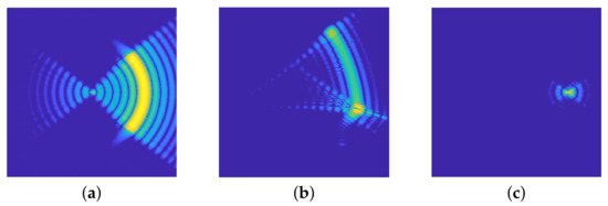
Figure 4.
The overfocused phenomenon of the AST: (a) SAR image of ideal trajectory; (b) SAR image of real trajectory; (c) SAR image after applying TAM to (b).
2.2. Analyses Based on the Proposed Parametric Motion Error Model
To explain the reason for the aforementioned overfocused phenomenon in Figure 4, we put forward the following proposition:
Proposition 1.
When the TAM is applied to the AST, the estimated motion error phases will be coupled with the arc-scattering phases, which are extremely related to the radius parameter of the AST; thus, the AST will be overfocused to a point target.
Proof.
As shown in Figure 3, the coordinates of any point P on an AST can be parametric expressed as follows:
where is the radius of the AST; are the coordinates of AST center C; is the angle between the straight line and the positive half axis of X. Similarly, the position of the radar platform at the azimuth time is:
where is the slant distance between the radar platform and the origin O at azimuth time ; is the angle between the radar platform and the X positive semi-axis at azimuth time . Then, the slant distance of the arc-scattering point P can be expressed as:
where is the distance from the radar trajectory to AST center C at the azimuth time , which is given by:
Thus, according to [39], if the radar observation angle includes the main lobe range of an AST, the imaging signal model of the AST can be expressed as:
where is the singh function; is the range time; ; is signal bandwidth; c is the speed of light.
According to (6), it is clear that the instantaneous scattering point of the AST is the intersection point of the AST center and radar. In other words, the arc-scattering point will slide with the movement of the radar. Note that at each azimuth time, all scattering points are fully illuminated. Due to coherent scattering, all scattering points will be coherently superimposed, which is equivalent to an instantaneous scattering point [40]. This means that the instantaneous scattering point is an equivalent point due to coherent scattering, while all scattering points are always illuminated. Therefore, the azimuth Doppler characteristics of the target scattering point still hold. As shown in Figure 3, when the radar platform is operating on the ideal trajectory and real trajectory, the phase histories of the AST, respectively, are:
where are the coordinates of the AST center C; and are the coordinates of the ideal and real radar trajectory at azimuth time , respectively; and are the slope distance from the radar platform to point P under the ideal and real trajectory, respectively; is the instantaneous scattering point of the AST at the azimuth time .
Therefore, according to the point-scattering model of the TAM, the estimated motion error phases of the AST are:
where is the phase history of point M; are the coordinates of the sliding scattering point of the AST at the center of the aperture.
It is clear that the estimated motion error phases of (9) are coupled with the arc-scattering phases in (6). The real motion error phases of sliding scattering points of the AST should be the difference between (8) and (7):
The difference between (9) and (10) is the arc-scattering phases caused by the sliding scattering model, which can be expressed as:
Once the above arc-scattering phases are utilized to compensate for the echo of the AST, it will become as below:
It can be seen that the echo is from the AST to the point M after compensating for the arc-scattering phases. In other words, the AST will be overfocused to a point target after adopting a TAM.
Then, we complete the proof. □
2.3. Problem Formulation
In the previous subsection, we analyzed that when the TAM performs on the AST, the estimated motion error phases will be coupled with the arc-scattering phases and the AST will be overfocused to a point target. The estimated motion error can be expressed as:
where represent high-order nonlinear motion error phases, and are arc-scattering phases. Note that both of these will change with the radar observation angle, i.e., they are both time-varying.
Suppose the number of radar azimuth points is N. It can be observed that the equation number of (13) is N, but there are unknowns. The equation is underdetermined and cannot be solved directly. Thus, it is important to reduce the number of unknowns.
A comparison of (10) with (1) reveals that the motion error of the sliding scattering point on the AST is the same as the point at the AST center. In other words, estimating the motion error of the AST center is equivalent to the scattering points on the AST. At the same time, according to (6), it can be observed that the echo of the AST and the echo of the AST center differ only in the slant range from the target parameters. According to the above analysis, one way to reduce the number of unknowns is to estimate the target parameter of the AST; thus, the number of unknowns is reduced to , where M is the parameter number of the target and in general.
Decoupling the motion error phase and the target scattering phase is an underdetermined problem, and the traditional autofocusing methods based on the point-scattering model, e.g., the method proposed in [41] (the TAMs method compared in this paper), will fail to solve this underdetermined problem. Moreover, since the sparse prior cannot be satisfied, the widely used sparse estimation methods cannot solve the above underdetermined problem, either.
Hence, in Section 3, we propose the SAR parametric autofocusing method with generative adversarial network (SPA-GAN) to estimate the target parameters and obtain the correct focused SAR image.
3. SAR Parametric Autofocusing Method with Generative Adversarial Network
To solve the problem in Section 2, we propose the SPA-GAN, whose flowchart is shown in Figure 5. The SPA-GAN is mainly composed of four parts: (1) a generator network module, (2) a discriminator network module, (3) a parameter estimation module, and (4) a motion error estimation and compensation module. In the following part, we will introduce the structures and principles of the above modules in detail.
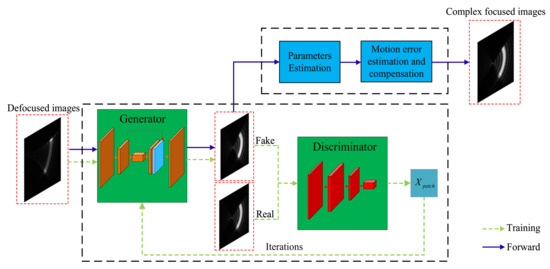
Figure 5.
The flowchart of the proposed SPA-GAN.
3.1. Generator Network Module
The generator network is trained to find the nonlinear mapping function for which can be expressed as:
where represents the AST focused distribution data; represents AST defocused distribution data; are the learning parameters of the generator network.
In this paper, as shown in Figure 6, we utilize the U-Net-shape network to construct the generator, whose structure is a symmetrical encoding–decoding architecture and is similar to the letter ‘U’ [42]. Due to the symmetrical structure, the input and output image sizes can be guaranteed to be consistent, and as the number of network layers goes deeper, the network can capture features of different scales. At the same time, the application of skip connection layers makes the output features contact the multi-scale information of the input features, which is helpful to restore the loss of input information caused by the downsampling of the encoder. This structure can help us find the deeper distribution relationship between input and output data.
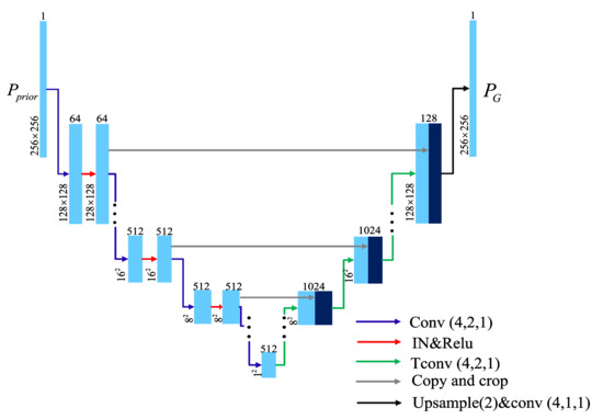
Figure 6.
Detailed structure of the generator network module. The and , respectively, denote the convolution operation and the de-convolution operation, where the size of the convolution kernel is set as , the stride is set as n, and the padding is set as q; represents the instance norm layer, and represents the network layer with an upsampling factor of 2.
In the encoder part, we increase the number of network layers to obtain deeper features. At the same time, we use to replace the combination of and to reduce the information loss caused by . Here, , respectively, denote the convolution operation, and the size of the convolution kernel is set as , the stride is set as n, and the padding is set as q. Therefore, the output of the encoder can be expressed as:
where is the output feature map of the encoder in the l-th layer; represents the weight of the l-th convolutional network layer of the encoder; is a combination of the convolutional layer , the normalization layer and the nonlinear layer in the encoder. can be expressed as:
As shown in Figure 6, the decoder and the encoder of the generator are mirrored and symmetrical. The output of the decoder is first upsampled by the transposed convolution, which can guarantee the feature map is the same size as the output of the encoder at the same layer. Then, we perform a concatenate operation with the output feature map of the encoder. Therefore, we can express the output of the l-th decoding layer as:
where and are the feature maps output by the encoder and the decoder in the -th layer, respectively; the final output is ; is the weight of the l-th convolutional network layers of the decoder; ∗ represents the matrix convolution operation; is the transposed convolution operation which can achieve upsampling; ⊕ is the matrix concatenate operation. After obtaining the real-valued through GAN, the parameters of the AST can be estimated. Thereafter, the scattering phase of the AST is obtained and compensated for based on (6) and the analyses of Section 2.3 in this paper. At this point, the final well-focused complex-valued image can be obtained by TAM.
3.2. Discriminator Network Module
The discriminator network is trained to distinguish the authenticity of the output data from the generator network. We define the input data of the discriminator network as , which are obtained by channel concatenate between the and the output data of the generator network or between the and the corresponding . Thus, can be written as:
where represents the channel concatenate operation.
The structure of our discriminator network is not the same as the original GAN [23], which only outputs a scalar about the authenticity of the input data. Instead, as shown in Figure 7, we adopt the discriminator network of the Patch-GAN in which the discriminator network outputs a matrix about the authenticity of the input data [25]. In this way, the discriminator can perform block discrimination on the input data so that the target can be discriminated from the high-frequency perspective. To be more specific, the block discriminant matrix output by the discriminator network is given by:
where N is the number of network layers; is the output feature map of the discriminator network in the -th layer; and are the output data of the discriminator, which is the authenticity matrix for the output data of the generator; is the weight of the N-th convolutional network layers of the discriminator network; is a combination of the convolutional layer , the normalization layer and the nonlinear layer .
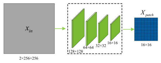
Figure 7.
The structure of the discriminator network module of the proposed SPA-GAN.
As for the loss function, in addition to the commonly used norm, we also utilize the norm to distinguish the authenticity from the low-frequency level. Thus, the discriminator network can distinguish from the two levels of the low frequency and high frequency of the image at the same time. In detail, the loss of the discriminator network consists of two parts:
where k is the ; is the true and fake label matrix of the input data for the discriminator, and it is the same size as . When the input data are , is an all-zero matrix, and is an all-one matrix when input data are ; is the regularization coefficient.
The main advantage of the Patch GAN proposed in this paper is that it can be discriminated from the low and high frequency of the image. According to (20), we can find that the second term is the norm of the image, which can be discriminated from the low frequency feature. The first item is the image block discrimination which can achieve the image high-frequency feature discrimination, owing to the number of samplings increasing. Furthermore, the low and high frequency discrimination of the image can be realized by controlling the regularization factor .
Through the zero-sum game between the generator in Section 3.1 and the discriminator in Section 3.2, an excellent generator can be trained.
3.3. Parameters Estimation Module
After sending a defocused image into a well-trained generator shown in Figure 6, the output of a well-focused image can be written as:
where is the output image of , is the input defocused image, and is the well-trained generative network.
Both the Hough transform and the Radon transform can detect line objects from images. The former is the discrete form of the linear parameter transformation, while the latter is the continuous form of the linear parameter transformation. In the process of this paper, the image can be binarized by a reasonable threshold setting, and then the target parameters can be quickly and accurately estimated by the Hough transform.
Once we obtain , we utilize the Hough transform (HT), which is one of the basic methods to identify geometric shapes from images in image processing [43], to extract the geometrical feature of the AST. The basic principle of HT is to use the duality of points and lines to transform a line in the original image space into a point target in the parameter space. In this way, the problem of detecting a given line target in the original image is transformed into a problem of finding a peak in the parameter space.
Thus, after applying the HT (marked as ), the estimations of the geometrical parameters of an AST can be given by:
where is the parameters of the AST; is the estimated radius of the AST; is the estimated coordinates of the AST center.
3.4. Motion Error Estimation and Compensation Module
After estimating the parameters of an AST, the arc-scattering phases can be obtained and compensated for according to the proposed model in Section 2. Note that the parameters estimation process is carried out in the image domain, and the compensation is processed in the echo domain sduch as the autofocusing methods based on minimum entropy (MEA) [44] and maximum sharpness (MSE) [45]. Once the arc-scattering phases are separated from the motion error phases, the TAM can be utilized to estimate the motion error phases. Finally, the estimated motion error is compensated for the original echo to obtain the well-focused image. The whole process can be expressed as:
where and represent the defocused echoes of the AST and the AST center, respectively; is the slope distance of AST; represents adopting TAM for motion error estimation; is the focused echo after compensating for the motion error phases.
In the autofocus processing flow, sometimes it is necessary to select the target to be processed. In this paper, it is to select the AST. Thus, the detection module, for example, can be embedded in the current front-end of SPA-GAN to realize the whole parametric autofocusing process.
3.5. Network Training
3.5.1. Training Data
The focused images of the ASTs are generated through the backprojection (BP) imaging algorithm, which can be specifically expressed as:
where is the echo of AST; denotes the BP imaging algorithm; are the aforementioned geometrical parameters of an AST. Then, we add a random phase within a reasonable range into the multi-frequency sine and polynomial form phase motion error to generate a corresponding defocused image , which can be represented by:
Therefore, a set of training set contains a pair of target focused and defocused images . Moreover, randomly changing the center coordinates , the radius , the central angle , and the center orientation angle of the AST within a certain reasonable range enhances the generalization of training data.
Note that the target parameters in the training samples are all randomly generated; therefore, all the training samples and test data in this paper are not the same or highly similar.
3.5.2. Training Skill
According to the training experience of [46], the discriminator network will slow down the learning speed of whole GANs when two networks have the same learning rate. During an actual training process, the update rate of the discriminator network is several times slower than the generator network, and this multiple is usually set to five. Hence, we use different learning rates for the generator network and the discriminator network, which can speed up the training procedure of the discriminator network.
3.5.3. Gradient Computation
We optimize the parameters of our generator and discriminator network by using the gradient-based algorithm, i.e., the Adam optimization algorithm, which is used with parameters , . The gradients of loss function with regard to parameters are calculated by backpropagation over the deep architectures. Due to the developments of the publicly available frameworks, e.g., TensorFlow and PyTorch, these complex gradient calculations can be fully automatically calculated. In this paper, we implement our method through PyTorch.
3.6. Network Convergence
The nonlinear mapping relationship between the sample data and the input data distribution is obtained through the zero-sum game of the generator network and the discriminator network. The ultimate goal of GAN is:
where
where G and D, respectively, are the generator network and the discriminator network; z is the input defocused AST data which satisfies distribution; is the distribution of G output; is the distribution of focused AST data. D and G are separately trained through iteration to obtain the distribution mapping between defocused and focused AST datas. According to [23], the above loss function can be trained to:
where represents KL divergence; represents JS divergence. Due to , when the G is optimal, , which is equal to . The minimum value of (28) is:
After a series of training iterations, is implemented, which is equal to . So the trained generator network can realize the mapping relationship from to . The training datasets are trained to obtain the mapping relationship: , and then the target parameters can be estimated from the focused image.
4. Numerical Experiments
In this section, first, some computer simulations are applied to validate the performance of our proposed SPA-GAN. Then, practical experiments in a microwave anechoic chamber are carried out to demonstrate the effectiveness of the proposed methods when applied to realistic targets. Finally, we adopt the public “Gotcha” data [47], which was released by the American Air Force Research Laboratory (AFRL) in 2007, to further demonstrate the effectiveness of our proposed method when applied to realistic scenarios.
4.1. Computer Simulation
4.1.1. The Scene That Contains an Arc Target
We place an arc target in the illuminated scene, the radius and central angle of the AST are and , respectively. The coordinates of the AST center is and the center orientation angle . Some radar parameters are listed in Table 1. Then, the BP imaging result with the ideal radar trajectory is shown in Figure 8a, which shows that the geometric information of the arc target can be clearly presented from the SAR image. The BP imaging result with the real radar trajectory is shown in Figure 8b, from which we can observe that the target has been deformed and defocused In addition, the geometric information of the target has been destroyed.

Table 1.
Simulation parameters.
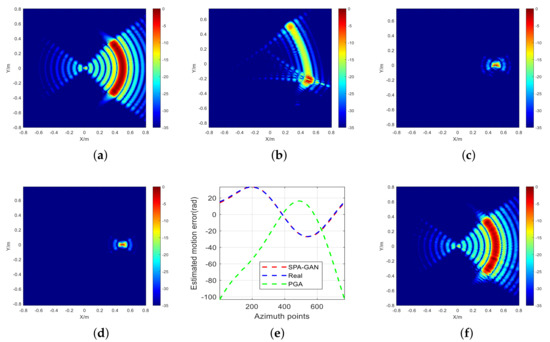
Figure 8.
Simulation experiment results of an arc target: (a) the BP result with the ideal trajectory; (b) the BP result with the real trajectory; (c) the PGA result; (d) the MSE result; (e) the estimated motion error of the proposed SPA-GAN, PGA and real motion error; (f) the proposed SPA-GAN result.
As shown in Figure 8c, the result of PGA becomes a point target that lost the real geometrical shape of the target completely. The reason is that the PGA is based on the point target model, which does not match the sliding scattering characteristics of the AST. Note that we converted the BP image to a polar coordinate domain to meet the conditions of using PGA [48]. The result in Figure 8c also verifies the proposed proposition in Section 2.2. In addition, the maximum sharpness estimation (MSE) [49] was applied to Figure 8b, and the result is shown in Figure 8d, which is similar to the PGA result because of the sliding scattering characteristics of the AST.
After sending the defocused arc image in Figure 8b into the proposed SPA-GAN, we can obtain the most important estimated result through the parameter estimation module of our SPA-GAN, i.e., the arc radius, given by = 0.508 m. Accordingly, in Figure 8e, we can see the estimated motion error of the proposed SPA-GAN is almost the same as the real motion error, and the estimated result of PGA is completely different from the real one. It should be noted that the experiments in this paper take sinusoidal error as an example, which does not mean that we can only deal with sinusoidal error. The final result is shown in Figure 8f, which shows that our proposed SPA-GAN can recover the same factual geometric information of the arc target as Figure 8a. Furthermore, compared with the results obtained by the ATMs shown in Figure 8c,d, the proposed SPA-GAN can cope with the autofocusing of the arc target accurately.
4.1.2. The Scene That Contains Multiple Targets
As shown in Figure 9, an arc target and three point targets were placed in the illuminated scene, and their parameter sets are listed in Table 2. Note that this does not mean that our method can only handle scenes that only contain a few simple targets. This is just to more easily show off the performance of our proposed method.
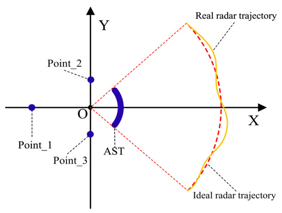
Figure 9.
The illuminated scene contains an arc target and three point targets.

Table 2.
The parameters of targets in Figure 9.
The BP imaging result of the ideal radar trajectory is shown in Figure 10a, and the corresponding result of the real radar trajectory is shown in Figure 10b. We can observe that the point targets and the arc target are defocused in the scene.
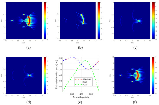
Figure 10.
Simulation experiment results of an arc target and three points; (a) the BP result with the ideal trajectory; (b) the BP result with the real trajectory; (c) the PGA resul; (d) the MSE result; (e) the estimated motion error of the proposed SPA-GAN, PGA and real motion error; (f) the proposed SPA-GAN result.
Figure 10c,d are the results of PGA and MSE for Figure 10b. It can be clearly observed that the arc target becomes a point target. At the same time, the point targets become arc-scattering targets because the scattering phases of the arc target are added to the point targets, which seriously change the original geometric information of the targets.
Then, after inputting the defocused arc image in Figure 10b into the proposed SPA-GAN, and according to the parameter estimation module of SPA-GAN, the radius of the arc target is estimated as = 0.505 m. Thus, in Figure 10e, we can see the estimated motion error of the proposed SPA-GAN is almost the same as the real motion error, and the PGA results are quite different. Finally, the final result is shown in Figure 10f, which demonstrates that the real geometric information of the multiple targets scene can be obtained through our proposed SPA-GAN directly.
4.1.3. The Scene That Contains Multiple Targets in a Noisy Environment
Based on the previous simulation experiments, to show the performance of the proposed SPA-GAN in a noisy environment, the image signal-to-noise ratio (SNR) reaches approximately 23 dB by adding specific complex Gaussian noise into the received echo.
The BP imaging result of the ideal radar trajectory is shown in Figure 11a. It can be seen that the noise destroys the details of the whole image. The BP imaging result of the real radar trajectory is shown in Figure 11b. which shows that point targets and the arc target are defocused in the scene. Figure 11c,d are the imaging results of PGA and MSE, which clearly show that the arc target becomes a point target and the point targets become arc-scattering targets at the same time.
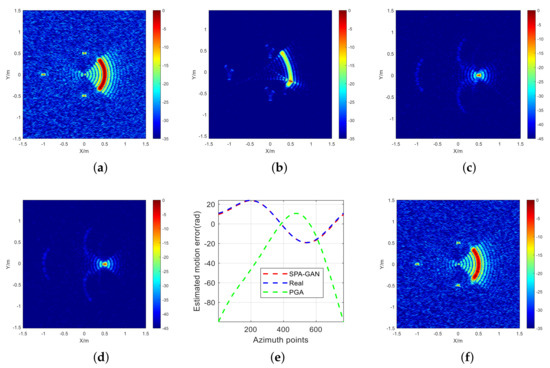
Figure 11.
Simulation experiment results of an arc target and three points for : (a) the BP result with the ideal trajectory; (b) the BP result with motion error; (c) the PGA result; (d) the MSE result; (e) the estimated motion error of the proposed SPA-GAN, PGA and real motion error; (f) the proposed SPA-GAN result.
Similarly, through our proposed SPA-GAN, we can obtain one of the estimated parameters as = 0.508 m. From Figure 11e,f, we can know that the estimated motion error of the proposed method is almost the same as the real motion error, and the geometric information of the image can be restored in a noisy environment, which shows that the proposed SPA-GAN is effective in a noisy environment.
4.1.4. The Scene That Contains Several ASTs with Different Shapes and Orientations
Based on the previous simulation parameters in Table 1, to demonstrate the effectiveness of the proposed method to deal with several ASTs with different orientations and shapes, several ASTs with different directions and radius were placed in the illuminated scene.
As shown in Figure 12c, similar to the previous three simulation experiment results, the several ASTs are all overfocused to point targets by the TAMs. In contrast, the proposed method is still valid for several ASTs with different shapes and orientations, as shown in Figure 12d, which demonstrates the generalization of the proposed method when handling several ASTs with different shapes and orientations as well.
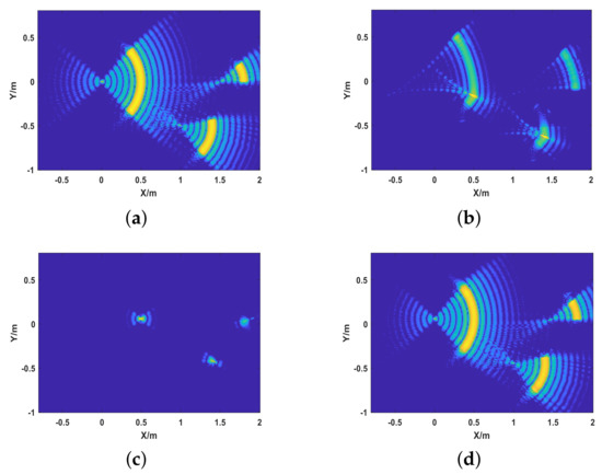
Figure 12.
Simulation experiments of different situations and methods; (a) the imaging result of ideal trajectory; (b) the imaging result of real trajectory; (c) the imaging result of TAMs; (d) the imaging result of the proposed method.
4.2. Performance Analyses
Based on the above simulation scenarios, this section will quantitatively evaluate performances from the signal SNRs and the levels of motion error.
4.2.1. Different SNRs
To quantitatively describe the performance of the proposed method under different SNRs, the image relevance (IR) is used to assess the ability of the complex information recovery with our proposed SPA-GAN, which is given by
where X and Y are the BP imaging result without motion error and the result of the proposed method, respectively. Equation (30) shows that the closer the IR is to one, the higher the image correlation becomes, which indicates that our method has a stronger ability to recover the complex image information. Conversely, the closer the IR is to 0, the lower the image correlation becomes.
In addition, to further measure the image structural similarity between the restored image and the true value image, the structural similarity (SSIM) is used for quantitative description [50], which is given by
where is the mean of X; is the mean of Y; is the variance of X; is the variance of Y; is the covariance of X and Y; and are the constants used to maintain stability; L is the dynamic range of pixel values; , . Equation (31) also shows that the closer the SSIM is to one, the more similar these two images become.
Keeping the simulation parameters the same as those in Table 1, we add some complex Gaussian noises of different amplitudes to the received signal echo to obtain noisy BP images with different SNRs.
After applying the proposed method, we can obtain the IR and SSIM curves with different methods at different SNRs as shown in Figure 13a.
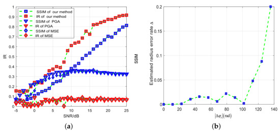
Figure 13.
Performance of our proposed method under the impact of two different nonideal factors in the simulation experiment. (a) The image relevance and structural similarity curves with different SNRs. (b) The estimated radius error rate curve with different levels of motion error.
Obviously, the proposed method can achieve better performance than the PGA and MSE methods. Even when SNR approaches 25 dB, the SSIM and IR for PGA and MSE still remain below 0.5, which means PGA and MSE cannot recover the structure of the target in the simulation experiments.
For the proposed method, as SNR increases, the IR and SSIM curves continuously increase. When the SNR is as low as 5 dB, the IR is only 0.37, and the SSIM is only 0.23. In that case, the reliability of the image information recovered by the proposed method is very low. The reason is that excessive noise leads to incorrect estimation of motion errors. When SNR reaches 20 dB, the IR increases to 0.87, and SSIM increases to 0.7 at the same time, which means the image information recovered by the proposed method is very close to the real result.
In addition, some typical values are listed in Table 3 and Table 4, which add the comparisons of the peak SNR (PSNR). PSNR is defined as follows:
where represents the mean square error of the current image and the reference image Y. H and W represent the length and width of the image, respectively; n is the number of bits per pixel, generally 8, that is, the number of pixel gray levels is 256. The unit of PSNR is dB, and the larger the value is, the smaller the distortion will be. In this paper, since more attention is paid to the structure of the AST, SSIM can better reflect the image structure restoration situation, but PSNR can also be used as an index reference for image restoration.

Table 3.
The metrics of proposed method at different SNRs.

Table 4.
The metrics of TAMs at different SNRs.
4.2.2. Motion Errors with Different Levels
To quantitatively describe the estimated accuracy of the proposed method under the motion error of different levels, the following estimated error rate of the most important target parameter, i.e., the radius of the target, is utilized:
where and are the estimated radius and real radius, respectively.
Keeping the simulation parameters the same as those in Table 1, we add some motion errors of different amplitudes to the radar trajectory to obtain defocused BP images with different motion errors. Through the parameter estimation module of the proposed SPA-GAN, the estimated radius error rate curve under different motion error levels is shown in Figure 13b. When the is within 120 radians, the estimated radius error rate is less than 0.05, in which case the estimated radius is effective for the next motion error estimation and compensation module of our SPA-GAN. Note that 120 radians represent 20 wavelengths, i.e., 60 cm, which satisfy the accuracy after inertial navigation of INS and IMU [51]. When the reaches 137 radians, the estimated radius error rate is 0.2, which means that the motion error is difficult to be accurately estimated under the circumstances. This is because the excessive motion errors lead to excessive dispersion of the AST energy, which leads to the failure of our SPA-GAN.
4.3. Practical Experiments
To further validate the effectiveness of our proposed SPA-GAN, the real-data experiments which contain a metal arc cylinder in a microwave anechoic chamber and the public real-data experiments released by the American AFRL were carried out.
4.3.1. Real-Data Experiment That Contains a Metal Arc Cylinder
As shown in Figure 14a, we placed a metal arc cylinder in the center of the solid foam column. We simulated the rotation of the radar platform by turning a 2-D turntable. The specific detail of the metal arc cylinder is shown in Figure 14b, and its parameters are listed in Table 5. The elevation angle was . The carrier frequency was 15 GHz. The bandwidth B was set to 3 GHz, and the azimuth angle was set to .
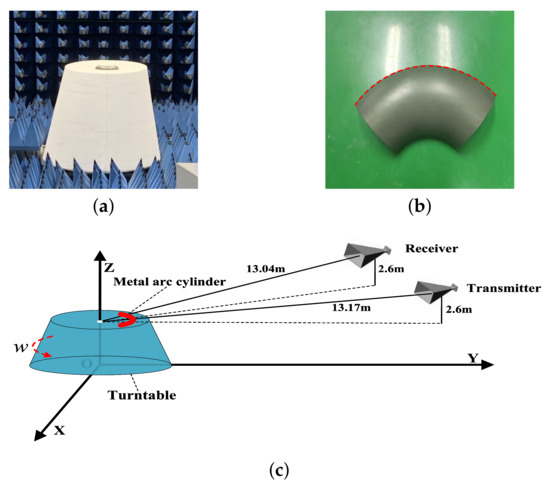
Figure 14.
Target and observation geometry for the real-data experiments: (a) metal arc cylinder on the turntable. (b) detail of metal arc cylinder. (c) observation geometry.

Table 5.
Target parameters in Figure 14.
Hereafter, the corresponding results are shown in Figure 15. The imaging result of the real radar trajectory is shown in Figure 15a. It can be seen that the metal arc target is defocused, and the geometric information is almost lost. As shown in Figure 15b,c, the results obtained by PGA and MSE show that the metal arc cylinder has been overfocused to a point target, which is the same as the simulation results in Figure 8c,d. Finally, the result of our proposed SPA-GAN is shown in Figure 15d. We can obtain the geometric information of the metal arc cylinder the same as Figure 14b, which means the proposed SPA-GAN effectively realized autofocusing during the real-data experiment.
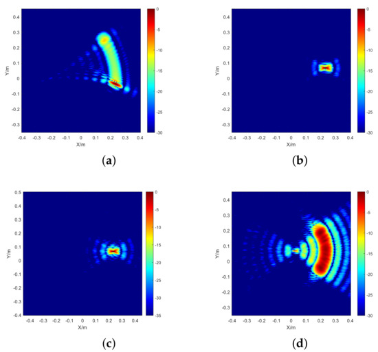
Figure 15.
Real-data experimental imaging results of the metal arc cylinder: (a) the BP result of the real trajectory; (b) the PGA result; (c) the MSE result; (d) the proposed SPA-GAN result.
4.3.2. Real-Data Experiment That Contains a Metal Arc Cylinder in Noisy Environment
To further prove the reliability of our proposed SPA-GAN in a noisy environment. We added Gaussian noise to the microwave anechoic chamber echo, which made the image reach dB. The corresponding results are shown in Figure 16. The BP imaging result of real trajectory is shown in Figure 16a. It can be seen that the image quality is much worse compared with Figure 15a, and the target is defocused. Figure 16b,c are the results of PGA and MSE for Figure 16a, respectively, which also shows that the metal arc cylinder has been overfocused to a point target. As shown in Figure 16d, although the result of our SPA-GAN is slightly different from the ideal result, the target geometry information can also be recovered correctly, which proves the proposed SPA-GAN is effective in the noisy environment.
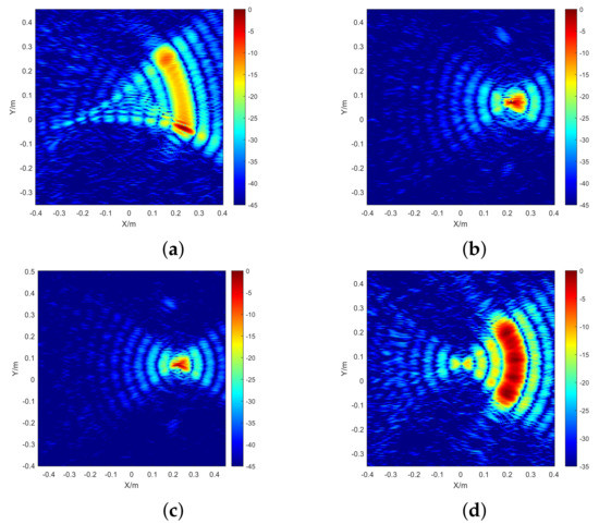
Figure 16.
Real-data experimental imaging results of the metal arc cylinder for : (a) the BP result of the real trajectory; (b) the PGA result; (c) the MSE result; (d) the proposed SPA-GAN result.
4.3.3. Publicly Released Airborne Data Which Contains Multiple Targets
The selected data for the following experiments are the publicly released HH polarized scattering echo of the artificials and vehicles (see Figure 17) with the corresponding experimental parameters listed in Table 6 [52]. There is a top hat with a radius of 1m and some vehicles in the scene (see Figure 17b,c in detail). In addition, to better show the effectiveness of our method when applied to “Gotcha”, we increased the motion error of the original data.
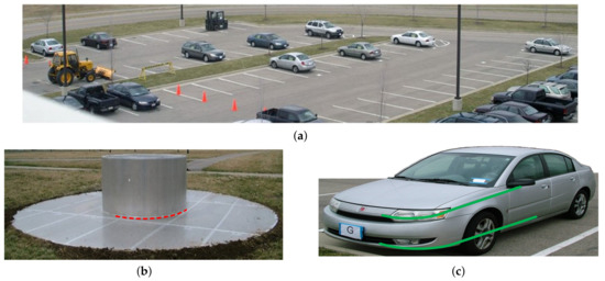
Figure 17.
The illuminated scene of publicly released data: (a) vehicles in the scene; (b) the top hat; (c) a vehicle.

Table 6.
Experimental parameters of publicly released airborne data.
The BP imaging results of real trajectory are shown in Figure 18a. It can be seen that the top hat is severely defocused, and the structure of the vehicle is destroyed. Note that by utilizing the YOLOv4-based AST detection module, as shown in Figure 18a, we succeeded in detecting the AST with a confidence of 0.94, even though the imaging scene is complex and diverse. Then, after applying the PGA method, as shown in Figure 18b, the top hat becomes a point target, and the structure of the vehicle is not corrected. Next, MSE is also applied, and the result is shown in Figure 18c. Unfortunately, the top hat has also become a point target, and the vehicle structure is still deformed.
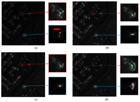
Figure 18.
Experimental results of publicly released data: (a) the BP result of real trajectory; (b) the PGA result; (c) the MSE result; (d) the proposed SPA-GAN result.
After utilizing our proposed SPA-GAN, we can obtain the result as shown in Figure 18d. The top hat in the imaging result becomes an arc target because of the limited angle of the radar trajectory and the arc-scattering characteristics, as mentioned in Section 2. Compared with Figure 17b,c, the autofocusing results of the proposed SPA-GAN are very close to the real structure of the targets, which demonstrate the effectiveness of our proposed SPA-GAN in practical scenarios.
As listed in Table 7 and Table 8, the IR and SSIM of the proposed method are much better than the TAMs, which verifies the effectiveness of the proposed method for recovering the true contours of arc-scattering targets. Moreover, the visual comparison of the enlarged imaging results in Figure 18 and the optical images of the top hat and car illustrate the effectiveness of the proposed method as well.

Table 7.
The metrics of different methods for the top hat area in Figure 18.

Table 8.
The metrics of different methods for the enlarged car area in Figure 18.
5. Discussion
In this paper, we proposed a SAR parametric autofocusing method with generative adversarial network (SPA-GAN) to solve the overfocused phenomenon. In the following, we will discuss the contributions and particularity of our proposed method in detail.
5.1. Contributions
After being validated by the simulations and real data experiments in Section 4, the contributions of our proposed method are threefold: (1) An arc-scattering parametric motion error model is established to analyze and explain the overfocused phenomenon of the AST. (2) Based on the proposed parametric motion error model, SPA-GAN is proposed to obtain the correct focused SAR image of distributed targets through solving the nonlinear coupling of the time-varying scattering phases and the real motion error phases. (3). A SAR parametric autofocusing framework, which contains a parametric motion error model, target parameter estimation and motion error phase estimation and compensation, is established to recover the real structure of a distributed target in the process of SAR autofocusing.
Additionally, the proposed network may also inspire other parameter estimation methods in the SAR field. For example, the proposed Patch GAN is mainly applied for physical parameter estimation, where the procedure or estimated parameters might potentially contribute to the processes in [36,37,38].
5.2. Network Generalization
When using SAR images of complex scenes as training samples, due to the few training samples, it is difficult for deep networks to learn various features of complex scenes, resulting in poor generalization. However, different from the traditional idea of using SAR complex scenes as training samples, the AST was chosen as training sample in our proposed method, which can allow a large amount of data to be generated. At the same time, through the analysis of scattering characteristics, an analytical scattering model of the AST was established under the influence of motion error. Based on this model, considering various non-ideal factors, we generated a large amount of training samples to achieve fine generalization and robustness., Furthermore, through combining a small amount of real data, the generalization and robustness can ultimately be guaranteed to have good generalization and robustness.
Accordingly, even though the same batch of simulation data was used for training in this paper, the proposed method still works well on multiple batches of different validation data containing targets with different shapes and orientations, which verifies that the proposed network has high robustness and generalization.
5.3. Network Structure
In order to discuss the advantages of the proposed GAN structure in this paper, some comparative experiments with other GAN networks were carried out. The network output and the true value of SSIM was applied to define the parameter estimation ability of the network. Finally, the result is given in Table 9. Compared with other GAN structures, the proposed GAN structure has better performance in parameter estimation.

Table 9.
Some comparative experiments with other GAN networks.
6. Conclusions
In this paper, through presenting the overfocused phenomenon of an AST by a TAM, the following problem is proposed: how to recover the real structure of the distributed target when it has been overfocused to a point target by a TAM. To solve this problem, a parametric autofocusing framework based on parametric modeling, parameter estimation, and motion error estimation was established.
First, to analyze the reason for the overfocused phenomenon, we proposed a parametric motion error model for the AST. According to the proposed model, we conclude that because the time-varying scattering phase and motion error phase were coupled, the anisotropic scattering phase and envelope of the target are compensated to be isotropic by the TAMs, which reduces the AST to a point target after autofocusing.
Next, after transforming the problem into estimating target parameters from a defocused image, we proposed SPA-GAN to estimate the target parameters from the defocused SAR image, so as to separate the scattering phase and the motion error phase. Afterward, by estimating the motion error phases of the whole trajectory with ATMs accurately, SPA-GAN can obtain a high-quality focused SAR image containing real structure of the distributed target successfully.
The results of simulations, real data, and publicly released data demonstrate that the proposed method can effectively solve the problem of overfocusing and obtain a high-quality focused image of the whole illuminated scene correctly. Furthermore, the experimental results verify that the proposed method has good robustness in many non-ideal situations.
Author Contributions
Conceptualization, Z.W. and Y.W.; methodology, Z.W.; software, Z.W. and L.L.; validation, Z.W.; formal analysis, Z.W., L.L. and Y.W.; investigation, Z.W. and X.M.; purces, L.L.; data curation, Z.W., Y.W. and X.M.; writing—original draft preparation, Z.W. and Y.W.; writing—review and editing, Z.W. and Y.W.; visualization, Z.W. and Y.W.; supervision, Z.W., Y.W. and X.M.; project administration, Z.W., Y.W. and T.Z. (Tianyi Zhang); funding acquisition, Z.D. and T.Z. (Tao Zeng). All authors have read and agreed to the published version of the manuscript.
Funding
This work was supported by the Key Program of National Natural Science Foundation of China (nos. 11833001 and 61931002) and the National Science Foundation for Distinguished Young Scholars under Grant 2020-JCJQ-ZQ-062.
Data Availability Statement
Not applicable.
Conflicts of Interest
The authors declare no conflict of interest.
References
- Soumekh, M. Synthetic Aperture Radar Signal Processing; Wiley: New York, NY, USA, 1999; Volume 7. [Google Scholar]
- Cumming, I.G.; Wong, F.H. Digital Processing of Synthetic Aperture Radar Data: Algorithms and Implementation [with CDROM] (Artech House Remote Sensing Library); Artech House: Boston, MA, USA, 2005. [Google Scholar]
- Soumekh, M. A system model and inversion for synthetic aperture radar imaging. In Proceedings of the International Conference on Acoustics, Speech, and Signal Processing, Albuquerque, NM, USA, 3–6 April 1990; pp. 1873–1876. [Google Scholar]
- Moreira, A.; Huang, Y. Airborne SAR processing of highly squinted data using a chirp scaling approach with integrated motion compensation. IEEE Trans. Geosci. Remote Sens. 1994, 32, 1029–1040. [Google Scholar] [CrossRef]
- Wang, G.; Bao, Z. The minimum entropy criterion of range alignment in ISAR motion compensation. In Proceedings of the Radar 97 (Conf. Publ. No. 449), Edinburgh, UK, 14–16 October 1997; pp. 236–239. [Google Scholar]
- Xi, L.; Guosui, L.; Ni, J. Autofocusing of ISAR images based on entropy minimization. IEEE Trans. Aerosp. Electron. Syst. 1999, 35, 1240–1252. [Google Scholar] [CrossRef]
- Wang, J.; Liu, X. SAR minimum-entropy autofocus using an adaptive-order polynomial model. IEEE Geosci. Remote Sens. Lett. 2006, 3, 512–516. [Google Scholar] [CrossRef]
- Fletcher, I.; Watts, C.; Miller, E.; Rabinkin, D. Minimum entropy autofocus for 3D SAR images from a UAV platform. In Proceedings of the 2016 IEEE Radar Conference (RadarConf), Philadelphia, PA, USA, 2–6 May 2016; pp. 1–5. [Google Scholar]
- Eichel, P.H.; Jakowatz, C. Phase-gradient algorithm as an optimal estimator of the phase derivative. Opt. Lett. 1989, 14, 1101–1103. [Google Scholar] [CrossRef]
- Jakowatz, C.V.; Wahl, D.E. Eigenvector method for maximum-likelihood estimation of phase errors in synthetic-aperture-radar imagery. JOSA A 1993, 10, 2539–2546. [Google Scholar] [CrossRef]
- Restano, M.; Seu, R.; Picardi, G. A phase-gradient-autofocus algorithm for the recovery of marsis subsurface data. IEEE Geosci. Remote Sens. Lett. 2016, 13, 806–810. [Google Scholar] [CrossRef]
- Wahl, D.E.; Eichel, P.; Ghiglia, D.; Jakowatz, C. Phase gradient autofocus-a robust tool for high resolution SAR phase correction. IEEE Trans. Aerosp. Electron. Syst. 1994, 30, 827–835. [Google Scholar] [CrossRef]
- Ao, D.; Wang, R.; Hu, C.; Li, Y. A sparse SAR imaging method based on multiple measurement vectors model. Remote Sens. 2017, 9, 297. [Google Scholar] [CrossRef]
- Chen, Y.X.; Guo, K.Y.; Mou, Y.; Sheng, X.Q. Scattering Center Modeling of Typical Planetary Landforms for Planetary Geomorphologic Exploration. IEEE Trans. Antennas Propag. 2021, 70, 1553–1558. [Google Scholar] [CrossRef]
- Keller, J.B. Geometrical theory of diffraction. JOSA 1962, 52, 116–130. [Google Scholar] [CrossRef]
- Potter, L.C.; Moses, R.L. Attributed scattering centers for SAR ATR. IEEE Trans. Image Process. 1997, 6, 79–91. [Google Scholar] [CrossRef] [PubMed]
- Akyildiz, Y.; Moses, R.L. Scattering center model for SAR imagery. In Proceedings of the Remote Sensing, 1999, Florence, Italy. International Society for Optics and Photonics. SPIE 2019, 3869, 76–85. [Google Scholar]
- LeCun, Y.; Bengio, Y.; Hinton, G. Deep learning. Nature 2015, 521, 436–444. [Google Scholar] [CrossRef]
- Goodfellow, I.; Bengio, Y.; Courville, A. Deep Learning; MIT Press: Cambridge, MA, USA, 2016. [Google Scholar]
- Krizhevsky, A.; Sutskever, I.; Hinton, G.E. Imagenet classification with deep convolutional neural networks. Adv. Neural Inf. Process. Syst. 2012, 25, 1097–1105. [Google Scholar] [CrossRef]
- Simonyan, K.; Zisserman, A. Very deep convolutional networks for large-scale image recognition. arXiv 2014, arXiv:1409.1556. [Google Scholar]
- He, K.; Zhang, X.; Ren, S.; Sun, J. Deep residual learning for image recognition. In Proceedings of the IEEE Conference on Computer Vision and Pattern Recognition, Las Vegas, NV, USA, 27–30 June 2016; pp. 770–778. [Google Scholar]
- Goodfellow, I.; Pouget-Abadie, J.; Mirza, M.; Xu, B.; Warde-Farley, D.; Ozair, S.; Courville, A.; Bengio, Y. Generative adversarial networks. Commun. ACM 2020, 63, 139–144. [Google Scholar] [CrossRef]
- Radford, A.; Metz, L.; Chintala, S. Unsupervised representation learning with deep convolutional generative adversarial networks. arXiv 2015, arXiv:1511.06434. [Google Scholar]
- Isola, P.; Zhu, J.Y.; Zhou, T.; Efros, A.A. Image-to-image translation with conditional adversarial networks. In Proceedings of the IEEE Conference on Computer Vision and Pattern Recognition, Honolulu, HI, USA, 21–26 July 2017; pp. 1125–1134. [Google Scholar]
- Zhu, J.Y.; Park, T.; Isola, P.; Efros, A.A. Unpaired image-to-image translation using cycle-consistent adversarial networks. In Proceedings of the IEEE International Conference on Computer Vision, Venice, Italy, 22–29 October 2017; pp. 2223–2232. [Google Scholar]
- Tulyakov, S.; Liu, M.Y.; Yang, X.; Kautz, J. Mocogan: Decomposing motion and content for video generation. In Proceedings of the IEEE Conference on Computer Vision and Pattern Recognition, Salt Lake City, UT, USA, 18–23 June 2018; pp. 1526–1535. [Google Scholar]
- Ledig, C.; Theis, L.; Huszár, F.; Caballero, J.; Cunningham, A.; Acosta, A.; Aitken, A.; Tejani, A.; Totz, J.; Wang, Z.; et al. Photo-realistic single image super-resolution using a generative adversarial network. In Proceedings of the IEEE Conference on Computer Vision and Pattern Recognition, Honolulu, HI, USA, 21–26 July 2017; pp. 4681–4690. [Google Scholar]
- Reed, S.; Akata, Z.; Yan, X.; Logeswaran, L.; Schiele, B.; Lee, H. Generative adversarial text to image synthesis. In Proceedings of the International Conference on Machine Learning, New York, NY, USA, 20–22 June 2016; pp. 1060–1069. [Google Scholar]
- Singh, P.; Komodakis, N. Cloud-gan: Cloud removal for sentinel-2 imagery using a cyclic consistent generative adversarial networks. In Proceedings of the IGARSS 2018—2018 IEEE International Geoscience and Remote Sensing Symposium, Valencia, Spain, 22–27 July 2018; pp. 1772–1775. [Google Scholar]
- Li, X.; Du, Z.; Huang, Y.; Tan, Z. A deep translation (GAN) based change detection network for optical and SAR remote sensing images. ISPRS J. Photogramm. Remote Sens. 2021, 179, 14–34. [Google Scholar] [CrossRef]
- Guo, J.; Lei, B.; Ding, C.; Zhang, Y. Synthetic aperture radar image synthesis by using generative adversarial nets. IEEE Geosci. Remote Sens. Lett. 2017, 14, 1111–1115. [Google Scholar] [CrossRef]
- Shi, X.; Zhou, F.; Yang, S.; Zhang, Z.; Su, T. Automatic target recognition for synthetic aperture radar images based on super-resolution generative adversarial network and deep convolutional neural network. Remote Sens. 2019, 11, 135. [Google Scholar] [CrossRef]
- Zhang, W.; Zhu, Y.; Fu, Q. Semi-supervised deep transfer learning-based on adversarial feature learning for label limited SAR target recognition. IEEE Access 2019, 7, 152412–152420. [Google Scholar] [CrossRef]
- Zhu, X.X.; Montazeri, S.; Ali, M.; Hua, Y.; Wang, Y.; Mou, L.; Shi, Y.; Xu, F.; Bamler, R. Deep learning meets SAR. arXiv 2020, arXiv:2006.10027. [Google Scholar]
- Huang, Z.; Yao, X.; Han, J. Progress and Perspective on Physically Explainable Deep Learning for Synthetic Aperture Radar Image Interpretation. J. Radars 2022, 10, 1–19. [Google Scholar]
- Niu, S.; Qiu, X.; Lei, B.; Ding, C.; Fu, K. Parameter extraction based on deep neural network for SAR target simulation. IEEE Trans. Geosci. Remote Sens. 2020, 58, 4901–4914. [Google Scholar] [CrossRef]
- Sica, F.; Gobbi, G.; Rizzoli, P.; Bruzzone, L. Φ-Net: Deep residual learning for InSAR parameters estimation. IEEE Trans. Geosci. Remote Sens. 2020, 59, 3917–3941. [Google Scholar] [CrossRef]
- Wang, Y.; Wen, Y.; Chen, X.; Kuang, H.; Fan, Y.; Ding, Z.; Zeng, T. Parametric reconstruction of arc-shaped structures in synthetic aperture radar imaging. Int. J. Remote Sens. 2021, 42, 7143–7165. [Google Scholar] [CrossRef]
- Guo, K.Y.; Li, Q.F.; Sheng, X.Q.; Gashinova, M. Sliding scattering center model for extended streamlined targets. Prog. Electromagn. Res. 2013, 139, 499–516. [Google Scholar] [CrossRef]
- Chen, L.; An, D.; Huang, X. A backprojection-based imaging for circular synthetic aperture radar. IEEE J. Sel. Top. Appl. Earth Obs. Remote Sens. 2017, 10, 3547–3555. [Google Scholar] [CrossRef]
- Ronneberger, O.; Fischer, P.; Brox, T. U-net: Convolutional networks for biomedical image segmentation. In Proceedings of the International Conference on Medical Image Computing and Computer-Assisted Intervention, Singapore, 18–22 September 2015; pp. 234–241. [Google Scholar]
- Illingworth, J.; Kittler, J. A survey of the Hough transform. Comput. Vision Graph. Image Process. 1988, 44, 87–116. [Google Scholar] [CrossRef]
- Wang, J.; Liu, X.; Zhou, Z. Minimum-entropy phase adjustment for ISAR. IEE Proc.-Radar Sonar Navig. 2004, 151, 203–209. [Google Scholar] [CrossRef]
- Morrison, R.L.; Do, M.N.; Munson, D.C. SAR image autofocus by sharpness optimization: A theoretical study. IEEE Trans. Image Process. 2007, 16, 2309–2321. [Google Scholar] [CrossRef] [PubMed]
- Zhang, H.; Goodfellow, I.; Metaxas, D.; Odena, A. Self-attention generative adversarial networks. In Proceedings of the International Conference on Machine Learning, Long Beach, CA, USA, 9–15 June 2019; pp. 7354–7363. [Google Scholar]
- Austin, C.D.; Ertin, E.; Moses, R.L. Sparse multipass 3D SAR imaging: Applications to the GOTCHA data set. In Proceedings of the Algorithms for Synthetic Aperture Radar Imagery XVI, International Society for Optics and Photonics, St. Asaph, UK, 5–7 June 2009; Volume 7337, p. 733703. [Google Scholar]
- Zhou, S.; Yang, L.; Zhao, L.; Bi, G. Quasi-polar-based FFBP algorithm for miniature UAV SAR imaging without navigational data. IEEE Trans. Geosci. Remote Sens. 2017, 55, 7053–7065. [Google Scholar] [CrossRef]
- Gao, Y.; Yu, W.; Liu, Y.; Wang, R. Autofocus algorithm for SAR imagery based on sharpness optimisation. Electron. Lett. 2014, 50, 830–832. [Google Scholar] [CrossRef]
- Wang, Z.; Bovik, A.C.; Sheikh, H.R.; Simoncelli, E.P. Image quality assessment: From error visibility to structural similarity. IEEE Trans. Image Process. 2004, 13, 600–612. [Google Scholar] [CrossRef]
- Xiaolan, Q.; Zekun, J.; Zhenli, Y.; Yao, C.; Bei, L.; Yitong, L.; Wei, W.; Yongwei, D.; Liangjiang, Z.; Chibiao, D. Key Technology and Preliminary Progress of Microwave Vision 3D SAR Experimental System. J. Radars 2022, 11, 1–19. [Google Scholar]
- Dungan, K.E.; Ash, J.N.; Nehrbass, J.W.; Parker, J.T.; Gorham, L.A.; Scarborough, S.M. Wide angle SAR data for target discrimination research. In Proceedings of the Algorithms for Synthetic Aperture Radar Imagery XIX.SPIE Defense, Security, and Sensing, 2012, Baltimore, Maryland, United States; SPIE: Bellingham, WA, USA, 2012; Volume 8394, pp. 181–193. [Google Scholar]
Publisher’s Note: MDPI stays neutral with regard to jurisdictional claims in published maps and institutional affiliations. |
© 2022 by the authors. Licensee MDPI, Basel, Switzerland. This article is an open access article distributed under the terms and conditions of the Creative Commons Attribution (CC BY) license (https://creativecommons.org/licenses/by/4.0/).