1. Introduction
High-resolution remote-sensing scene-image classification, as a fundamental task in remote-sensing-image understanding, has received increasing attention in the past few years [
1,
2,
3]. Thanks to the development of satellite and remote-sensing technologies, remote-sensing scene-image classification plays an important role in real-life applications, such as urban construction and planning [
4,
5], land cover and land use (LCLU) [
6], vegetation mapping [
7], remote monitoring and intelligent decision making [
8,
9].
Difficulties in the study of remote-sensing scene-image classification are influenced by the characteristics of the images themselves. Compared to natural images, remote-sensing scene images contain more objects at different scales because they are taken from a bird’s eye view. As shown in
Figure 1a, remote-sensing images often contain many objects which are diverse in size. As shown in
Figure 1b, objects in natural images are usually medium-sized and centered, but in remote-sensing images, objects generally have multiple scales and show a dense distribution at any location in the image. In addition, remote-sensing images often contain a large amount of useless background information due to the angle of imaging, making it more difficult to capture key object features than natural images. In addition, the remote-sensing scene images contain a large number of similar scenes, and have the characteristics of small inter-class differences and large intra-class differences. As shown in
Figure 2, the categories in (a) are the same, but their architectural styles are obviously different, and the shapes of the main objects are not similar; the categories in (b) are different but very similar, such as “runway”, “freeway”, “railway” and “intersection”, which are sometimes difficult to distinguish with the naked eye. Another example involves “terrace”, “meadow”, “wetland” and “forest”, which mostly contain similar or identical objects, but they have completely different semantic labels. The above problems pose difficulties for accurate classification of remote-sensing scene images.
The early research methods are mainly based on low-level features, which represent the features of remote-sensing scene images by selecting different feature description operators. Some of the widely used methods include SIFT [
10], CH [
11], HOG [
12], GIST [
13] and LBP [
14]. However, with the rapid development of remote-sensing imaging technologies and platforms, the internal information contained in remote-sensing images is becoming more and more complex, and a single shallow feature is no longer applicable. To overcome the limitations of low-level feature description, the researchers proposed a method based on mid-level features. This type of approach obtains global features by encoding the extracted features (such as BoVW [
15], LDA [
16] and pLSA [
17]). However, these methods rely on a large amount of a priori information and sparse local features, and thus have limited ability to characterize remote sense images.
With the rapid development of deep learning methods (high-level features) since 2012, deep CNN models have become able to automatically learn and extract representative features from given data, and have achieved many impressive results in several fields [
18]. Compared with traditional feature extraction methods, deep learning methods have stronger recognition and feature description capabilities [
19]. Remote-sensing scene-image classification methods based on deep learning can be broadly classified into three categories, namely, fine tuning, full training and using a CNN as a feature extractor. The fine-tuning-based methods usually target CNN models pre-trained on large natural-image datasets beforehand, and use remote-sensing image datasets. CNN models require a large amount of data for training to reach their true potential, but remote-sensing datasets have the problem of small samples, so fine-tuning-based methods are generally effective. Full-training-based methods usually redesign the CNN structure based on remote-sensing scene-image features or improve the currently available superior models [
20,
21,
22]. The new model can extract key features directly from remote-sensing scene images, and thus works better than existing models such as VGGNet [
23], AlexNet [
24] and ResNet [
25]. Using a CNN as a feature extractor usually fuses multiple layers of features from a CNN model to obtain a more comprehensive feature representation map [
26,
27,
28,
29]. Although such methods outperform existing CNN models, they require CNN models that have already been trained on remote sensing datasets, and thus they lack flexibility.
Although the CNN has achieved some good results in the study of remote-sensing scene-image classification, the following problems still exist:
(1) Insufficient description of key semantic feature representations: The remote-sensing scene-image contains many objects or redundant backgrounds inside the image that are not related to labels, and also has the characteristics of large intra-class differences and small inter-class differences, but the CNN focuses on global features, which are easily disturbed by useless information and affect the final performance.
(2) Too many parameters make it difficult to train: Although the deeper CNNs have stronger feature representation capabilities, the small sizes of remote-sensing scene-image datasets tend to cause parameter redundancy, resulting in low accuracy. Meanwhile, the problem of gradient disappearance easily arises during the training process, which generates a high computational cost.
(3) Loss of shallow features: Although the discriminative power of deep features is stronger, retaining shallow features is more helpful to enriching the diversity of features. For remote-sensing scene images with complex spatial information, retaining shallow features is more helpful to describing different spatial structures and improving the final classification performance.
In recent years, multiple-instance learning (MIL) is often combined with a CNN. This combined approach can effectively distinguish the local semantic information associated with the scene labels [
30]. MIL was originally designed for drug activity prediction [
31]. Its effectiveness has since also been demonstrated in a range of computer-vision tasks, such as image recognition [
32], saliency detection [
33] and target detection [
34]. In MIL, training samples are specified as bags, each containing multiple instances, each with a predefined semantic label. A bag is labeled as a positive bag if it contains at least one positive instance, and vice versa. In general, there are no specific instance labels, and each instance can only be judged to belong to or be deployed in one bag category [
35], which makes MIL well suited for learning from weakly labeled data [
36,
37]. In the past few years, the combination of MIL and trainable CNNs has become a new trend. For example, Wang et al. [
36] used max pooling and mean pooling to aggregate instance representations in the network. However, this method is applicable to medical images or natural images, and does not adapt to create remote-sensing scene maps that contain complex spatial information.
To solve the above problems, this paper proposes a framework for remote-sensing scene-image classification based on the CNN and MIL. The main objectives include the following.
(1) Improved utilization of shallow features: Deep CNNs usually cannot retain shallow features, but shallow features help to improve feature diversity and enhance the performance of the final classification decision. Therefore, our model should effectively improve the feature reuse rate, improve feature propagation and make full use of the limited samples of remote-sensing scene images.
(2) Enhance the extraction of key features: The commonly used deep CNN models are inadequate in key local feature extraction. Since remote-sensing scene images contain a large amount of redundant background information and have high inter-class similarity, our model needs to improve the feature representation of key objects.
(3) Improved parameter utilization: Although increasing the depth of the CNN model helps to extract deeper features with more discriminative rows, it can easily cause parameter redundancy and overfitting. Therefore, our model should minimize the parameters while ensuring the feature extraction capability of the image-depth semantic information.
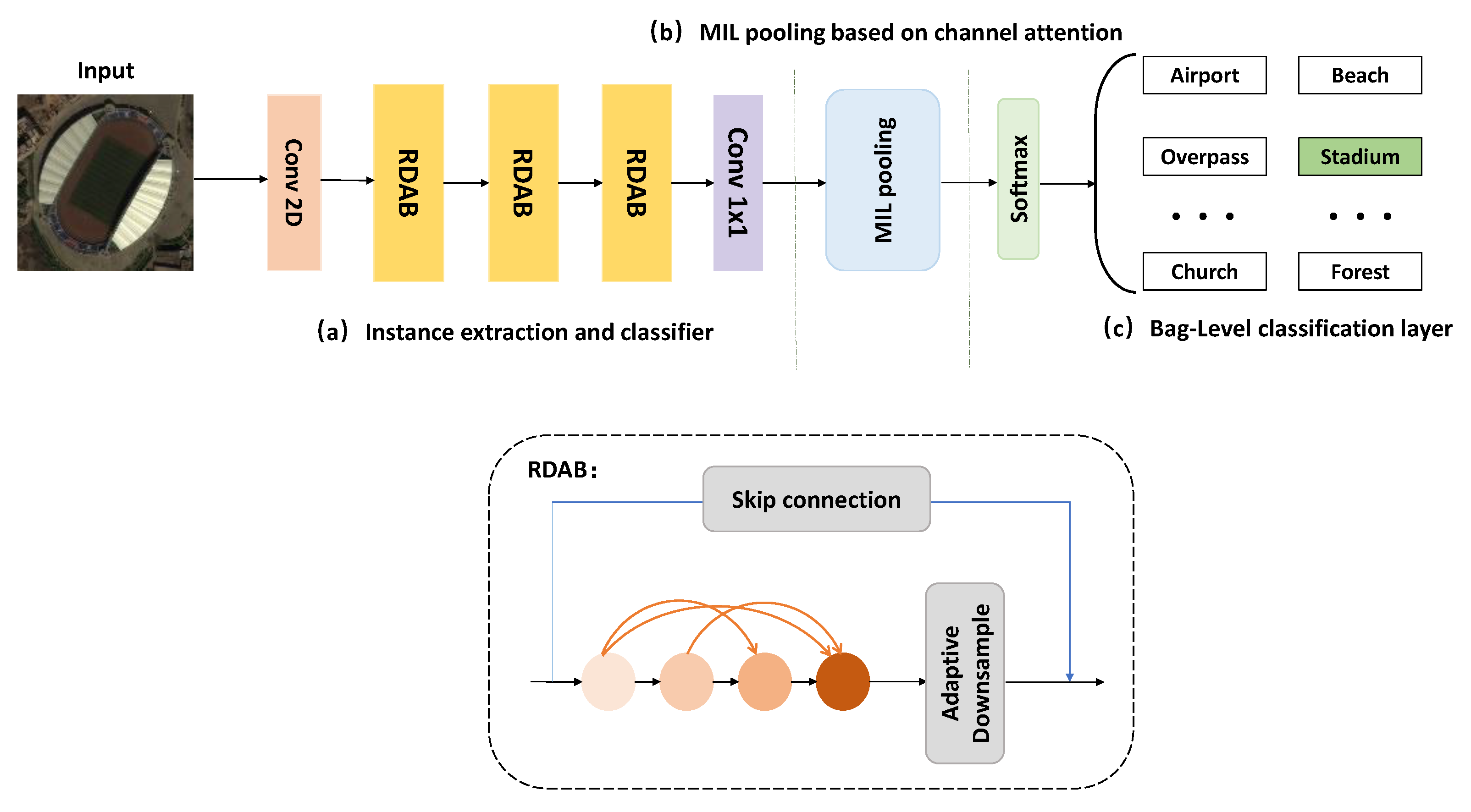
In summary, we first constructed a feature extraction module, RDAB, based on local residuals and dense connectivity, and converted the extracted features into local instance vectors. Then, the correlation weights were generated by aggregating the instance information through MIL pooling based on channel attention. Finally, the whole network is constrained by a cross-entropy loss function, so that the whole model outputs the final result directly under the supervision of bag-level labels.
The main contributions of this paper are as follows.
(1) We constructed an end-to-end lightweight network, MILRDA, for remote-sensing scene-image classification. Additionally, it has much smaller parameters and computational complexity compared to existing CNN models.
(2) We constructed the feature extraction module RDAB with local residuals and dense connections, which performs feature reuse and retains shallow features, which helps the network generate more discriminative information.
(3) The constructed MIL pooling based on channel attention and aggregating relevant instances, helps to suppress redundant background information of remote-sensing scene images while highlighting major instance weights and outputting prediction results directly under the supervision of bag-level labeling.
The rest of the article is organized as follows.
Section 2 introduces our proposed framework and describes its component parts in detail.
Section 3 describes the experimental results and compares them with those of other methods. In
Section 4, we discuss the proposed approach.
Section 5 summarizes the proposed method.
2. Methodology
Figure 3 shows the architecture of the proposed MILRDA method. MILRDA consists of three parts: (1) instance extraction and classifier, (2) MIL pooling and (3) a bag-Level classification layer. In this framework, we first extract features with the proposed convolution module and then feed the extracted features into the instance-level classifier to obtain instance-level feature vectors. The instance-level classifier here is made up of a series of
convolutions that are proportional in number to the number of remote-sensing scene images (for example, the UCM dataset corresponds to 21 convolutional groups, and the AID dataset corresponds to 30). Then, we use the proposed MIL pooling with channel attention to obtain the bag-level class probabilities. Finally, the true labels of the scene images are predicted by the softmax classifier. The network as a whole creates an end-to-end structure.
For remote-sensing scene classification tasks, each image in a training set
T is converted into a collection of local patches, which are referred to as instances. Let
denote each local patch that maps to the class label
of instance
through the instance-level classifier
h; each instance
is a local piece of image
. Then, the instance label is changed into an image (bag) label under the common MIL assumptions, which are based on the MIL pooling function
, denoted as:
This indicates that the negative image has solely negative patches, whereas the positive image has at least one positive patch. Since the instance-level label is an unknown hidden variable during the training process, it is crucial to establish the image-to-instance mapping h, and to establish the that transforms the instance label to the bag label. Deep convolutional neural networks have shown powerful capabilities in the field of computer vision, and we constructed a deep CNN to learn hidden variables, and the pooling function is a module based on channel attention to better highlight local key regions of images under class label supervision.
2.1. Instance Extraction and Classifier
Scene classification performance is somewhat impacted by the influence of feature extraction. Stronger feature representation may be attained with deeper CNN structures; however, these structures also come with issues, including gradient disappearance, parameter redundancy and challenging training [
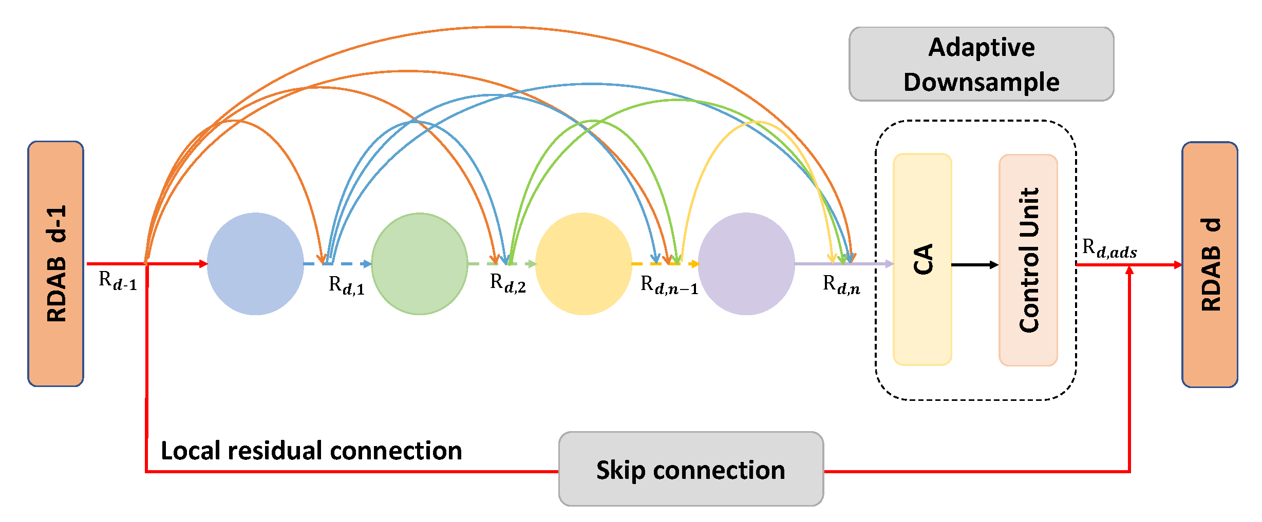
38]. We built a residual dense attention block (RDAB) for feature extraction to solve this problem and transformed it into an instance feature vector. The complete structure of the block is shown in
Figure 4. It consists of a dense connection layer, an attention-based adaptive downsampling layer and local residual connection.
(1) Dense Connection Layer
It is known that deep neural networks can be optimized with dense connections for more efficient feature extraction [
39]. When training deep neural networks, a large number of trainable parameters are often required, but the small data size of remote-sensing-image datasets makes it difficult to train the networks effectively. The densely connected structure provides feature reuse, which to some extent mitigates the remote sensing datasets’ limited sample learning difficulty and boosts training effectiveness. The output feature maps from each layer during feature extraction can be used as inputs for all succeeding layers. We set the number of densely connected layers in the three RDABs to four for multi-level feature representation, which makes the network structure more organized. The dense connection layers consist of
and
convolution operations; let
be the input of the
d-th RDAB, and
stands for the output of the
n-th dense connection layer in the
d-th RDAB. The whole process of dense connection can be expressed as:
where
H denotes the convolution; BN, ReLU three consecutive composite functions;
denotes the successive operations of the feature map generated by the
th RDAB. The output feature map channel of
is
, where
is the input feature map channel of
, and
N is the growth rate of each dense connection layer.
(2) Attention-Based Adaptive Downsampling
The final output number of feature channels, after the features have passed through numerous tightly coupled layers, is the total of the earlier channels. To ease the network training burden and improve the features while drawing attention to the weights of important regions, we created an attention-based control unit called the adaptive downsampler. The original control unit (CU) consists of
convolution and average pooling [
39]. We placed a coordinate attention (CA) at the front end to highlight key discriminative features while reducing the number of feature channels and improving the efficiency of sampling. CA is a light and high-efficiency attention mechanism that embeds location information into the channel [
40]. Compared with the original channel attention mechanism, CA allows lightweight CNNs to acquire critical information at a larger scale. Referring to the experimental procedure of CA, this mechanism is introduced into the constructed residual densely connected module in this paper. CA generates attention weights by encoding channel information in horizontal and vertical coordinates, which are then aggregated. The complete structure is shown in
Figure 5, which contains two parts: coordinate information embedding (CIE) and coordinate attention generation (CAG).
CIE: Encoding using the global pooling makes it difficult to retain location information [
41]. Therefore, the global average pooling is first decomposed into a bi-directional average set of channels, and the association between long distances is obtained by location information. The outputs of the
c-th channel with height
h and width
w are expressed, respectively, as:
where
W and
H denote the width and height of the feature map F, and
represents the pixel value of c-th channel in the feature map. This operation compresses all pixels of each channel into a single feature vector that gets long dependencies along both directions, helping the network to better capture important information.
CAG: The features obtained in both directions are concatenated and then channel compressed by a shared 1 × 1 convolutional layer:
where
represents the concatenation operation for manipulating the spatial dimension, and
represents the non-linear and BatchNorm, which encode spatial information in both horizontal and vertical directions. The resulting tensor is then split into its component pieces,
and
, and its dimensionality is changed using convolution operation, yielding
where
and
represent two 1 × 1 convolutional operations that convert
and
into a tensor with the same number of channels as the input features.
is the sigmoid activation function. The outputs
and
are re-weighted and fused as attention weights with the original input features to get
, which can be represented as:
where
denotes the
c-th channel of the input feature map. In the
H and
W directions,
and
are the attention weights for the
i-th and
j-th positions. The output flow of the whole adaptive downsample can be expressed as:
where
is the output of adaptive downsample, and
W is the operation of CA and CU.
(3) Local Residual Connection
To further ensure that the feature information transmitted by RDAB is not lost and to improve the efficiency and use of the transferred features, driven by the idea of RDN [
42], a local residual connection is added between the RDAB input and output. This skip connection technique can address the issue of gradient disappearance in deep networks and achieve the fusion of local features of densely connected blocks, which to some extent increases the variety of features. The
convolution is utilized for the local residual connection in order to preserve the consistency of the RDAB input and output dimensions, and the output
of the
d-th RDAB can be written as follows:
The output of RDAB can connect with all preceding layers and directly access the original input features, which not only increases feature reuse but also creates implicit deep supervision.
(4) Instance-level Classifier
For remote-sensing scene-image classification tasks, when MIL is introduced, an instance-level classifier needs to be built to sample the local image patches [
43]. Specifically, in MILRDA, the image is obtained as a multi-channel feature map after a series of convolutional-feature-extraction operations. Each position on the feature map corresponds to a local feature vector. The feature maps are fed into a
convolution layer consistent with the number of scenes needed to build an instance-level classifier. Additionally, bag-level semantic labels can be given to the local instances in each feature map.
2.2. MIL Pooling Based on Channel Attention
The MIL pooling converts the instance feature vector to a label at the bag level. The remote-sensed scene images contain many occurrences unrelated to the bag level labels and are available in various sizes. In other words, the instances in the feature map can cover one or more categories (channels). Therefore, there is nonlinear dependence between the different channels. To solve this problem, we constructed MIL pooling based on channel attention [
41] that combines CNN and MIL to suppress irrelevant instances while highlighting important regions. The module structure is shown in
Figure 6.
The MIL pooling based on channel attention first initializes channel weights by global average pooling of
u:
Then, the nonlinearity between different channels is captured by two fully connected layers:
where
is the sigmod function and
is the ReLU function to limit the range of instance weights. There is a skip connection between the output of the input and the sigmoid layer. The final outputs, feature maps
, are obtained by channelwise multiplication:
After obtaining the instance weights, the class-score vector
at the bag level is calculated by weighted average. Each channel of
P represents an image class. The probability of the input image belonging to class
c is
.
2.3. Bag-Level Classification
The softmax classifier receives the output bag-level scores and converts them into conditional probabilities for each class. Then, we calculate the loss between the bag level probability
and the true label
by the cross-entropy loss function:
Here, the loss between the bag-level prediction and the true label is obtained by direct minimization of the global optimization [
43].


