Abstract
High-Resolution Wide-Swath (HRWS) is an important development direction of space-borne Synthetic Aperture Radar (SAR). The two-dimensional spatial variation of the Doppler parameters is the most significant characteristic of the sliding spotlight space-borne SAR system under the requirements of HRWS. Therefore, the compensation of the two-dimensional spatial variation is the most challenging problem faced in the imaging of HRWS situations. The compensatory approach is then proposed to address this problem in this paper. The spatial distribution of the Doppler parameters for the HRWS space-borne SAR data in the sliding spotlight working mode is firstly analyzed, based on which a Spatial-Variant Equivalent Slant Range Model (SV-ESRM) is put forward to accurately formulate the range history for the distributed target. By introducing an azimuth-varying term, the SV-ESRM can precisely describe the range history for not only central targets but also marginal targets, which is more adaptive to the HRWS space-borne SAR requirements. Based on the SV-ESRM, a Modified Hybrid Correlation Algorithm (MHCA) for HRWS space-borne SAR imaging is derived to focus the full-scene data on one single imaging processing. A Doppler phase perturbation incorporated with the sub-aperture method is firstly performed to eliminate the azimuth variation of the Doppler parameters and remove the Doppler spectrum aliasing. Then, an advanced hybrid correlation is employed to achieve the precise differential Range Cell Migration (RCM) correction and Doppler phase compensation. A range phase perturbation method is also utilized to eliminate the range profile defocusing caused by range-azimuth coupling for marginal targets. Finally, a de-rotation processing is performed to remove the azimuth aliasing and the residual azimuth-variance and obtain the precisely focused SAR image. Simulation shows that the SAR echoes for a 20 km × 20 km scene with a 0.25 m resolution in both the range and azimuth directions could be focused precisely via one single imaging processing, which validates the feasibility of the proposed algorithm.
1. Introduction
Synthetic aperture radar (SAR) is a powerful remote sensing technology which can obtain the two-dimensional image and relevant information of the Earth’s surface regardless of weather conditions [1,2,3,4]. Since the successful launch of the first space-borne SAR SEASAT-1 in 1978 [5,6], significant progress has been made in this area in terms of hardware and the imaging algorithms. Nowadays, high-resolution and wide-swath have become an important direction for the design of the new generation space-borne SAR [7,8,9,10]. For example, the TerraSAR-X Next Generation (TSX-NG) will allow a high spatial resolution down to 0.25 m and a 5 km swath in both azimuth and range directions [11,12,13]. This has also posed new challenges for the imaging processing. In order to obtain such a high resolution in azimuth direction, a much larger synthetic aperture is required, and the conventional time-invariance assumption no longer holds. Therefore, the conventional processing methods cannot meet the requirement of HRWS in sliding spotlight space-borne SAR. Firstly, the conventional range models fail to describe the actual range history of the distributed target. Secondly, the spatial variation of the Doppler parameters for targets in the same range cell becomes non-negligible, which means that their echoes cannot be focused via a single processing directly.
Due to the curvature of the satellite orbit and the rotation of the Earth, the range history of the space-borne SAR data is quite complex. Some range models have already been proposed to formulate the range history of space-borne SAR in a concise form. The Equivalent Squint Range Model (ESRM) or the Hyperbolic Range Equation Model (HREM) is the most well-known one [14,15], which assumes that the satellite has a straight path and a constant velocity. As the resolution of the space-borne SAR and consequently the synthetic aperture time increase, some high order range models have been established. The fourth-order Doppler range model (DRM4) [16,17,18] is derived by expanding the range history in a Taylor series and keeping terms up to the fourth order. In [19], a Modified Equivalent Squint Range Model (MESRM) is developed by introducing the equivalent radar acceleration into the conventional range model ESRM, which can not only describe the actual range history from first-order term to fourth-order term but also partially compensate the higher-order term and can therefore handle the higher resolution conditions. The precise focusing of space-borne SAR echo data with a resolution of 0.25 m is achieved in [19] by adopting the MESRM. However, in the HRWS space-borne SAR, the aforementioned range models can only match the range history for the point at the scene center, whereas for the azimuth marginal point, a non-negligible range error occurs, which results in the degradation in the imaging quality. Therefore, the establishment of a proper range model that can formulate the range history for the distributed targets is required in the HRWS space-borne SAR.
Another challenge faced in the HRWS space-borne SAR imaging is the two-dimensional spatial variation of the Doppler parameters. In the air-borne SAR, the Doppler parameters are identical for targets appearing in the same range cell, which could be called azimuth-invariance. This assumption is the basis for various frequency domain imaging algorithms, such as the Range Doppler Algorithm (RDA) [20,21], the Frequency Scaling Algorithm (FSA) [14,22], the Chirp Scaling Algorithm (CSA) [23,24,25], and the High-order Hybrid Correlation Algorithm (HHCA) [19], which can achieve the batch processing of the target echoes in the same range cell. In the HRWS space-borne SAR, however, this assumption no longer holds, which means that the azimuth marginal targets will suffer from defocusing when the conventional frequency domain algorithms are directly utilized in the imaging. Hence, the azimuth variance of the Doppler parameters should be dealt with before employing these frequency domain algorithms. In order to handle this issue, an azimuth-time resampling method in Joint Time-Doppler Resampling Algorithm (JTDRA) is proposed in [26], which could equalize the Doppler Frequency Modulation Rate (DFMR) by the scaling of the azimuth time. However, the non-linear resampling of the azimuth axis needs an interpolation process which is fairly time consuming, and the precision is also limited by the length of the interpolation kernel. In [27], a Doppler phase perturbation method is firstly proposed to equalize the azimuth-variant Doppler parameters for the bi-static air-borne SAR. The implementation of the Doppler phase perturbation requires only complex multiplications, which could achieve both high efficiency and good precision. In [28,29], the Doppler phase perturbation method is introduced to the space-borne SAR imaging with meter level resolutions based on the conventional range models. For the HRWS space-borne SAR, however, the characteristic of the two-dimensional spatial variation is much more complex than that in the medium resolution case, and the derivation and expression of the perturbation function should be adapted to the HRWS case and the new range model.
The spatial variance of the target echoes in the range direction behaves in the range-dependent DFRM and Range Cell Migration (RCM). In order to correct the range-variant RCM of the target echoes across different range cells, typically, a Chirp Scaling (CS) method [23,24,25] is performed which can eliminate the linear differential RCM through complex multiplications. When the resolution increases, the non-linear differential RCM becomes significant, and the Nonlinear Chirp Scaling (NCS) algorithm [30,31,32] is correspondingly proposed. However, when the resolution further increases, the precision of the NCS similarly cannot meet the requirement, and meanwhile, the NCS will introduce high-order modulations to the range phase, which could cause the degradation of the range profile for the imaging result.
In this paper, the precision of the conventional range models for HRWS space-borne SAR working in the sliding spotlight mode is analyzed for both the central target and the marginal targets. Then, the two-dimensional spatial variation characteristic of the Doppler parameters is studied, which illustrates that the DFMR variation is approximately proportional to the azimuth position of the target. Based on the analysis, a Spatial-Variant Equivalent Slant Range Model (SV-ESRM) is established for the requirement of the HRWS space-borne SAR. By introducing an additional spatially variant term to the MESRM, the SV-ESRM can precisely describe the range history for not only the central target but also the marginal targets. Based on the SV-ESRM, a Modified Hybrid Correlation Algorithm (MHCA) is proposed for the HRWS space-borne SAR imaging. Firstly, the sub-aperture method is adopted to eliminate the azimuth spectrum aliasing of the target echoes. Secondly, a Doppler phase perturbation method is performed to equalize the DFRM for the same range cell targets. Next, an advanced high-order hybrid correlation operation is employed to accomplish the precise differential RCM correction and Doppler phase compensation. A range phase perturbation method is also performed to equalize the range frequency modulation rate across different range cells and eliminate the defocusing in range profile for marginal targets. Finally, a de-rotation processing is performed to remove the azimuth aliasing and the residual azimuth-variance, and the precisely focused SAR image of the whole scene is then acquired. Simulation shows that the SAR echo signal for a scene with a 0.25 m resolution in both range and azimuth directions could be focused precisely through one single imaging processing, which demonstrates the accuracy of the SV-ESRM and the feasibility of the proposed algorithm. As a summary, Table 1 categorizes the distinctive characteristics of the aforementioned algorithms as well as the proposed MHCA. The mathematical notations adopted in this paper are given in Table 2.

Table 1.
Comparison between the related algorithms.
Table 2.
The mathematical notations.
The rest of this paper is organized as follows: The analysis of the spatial-variant system and the establishment of the spatial-variant signal model for HRWS space-borne SAR are given in Section 2. The details of the proposed algorithm are displayed in Section 3. The stimulations and results are illustrated in Section 4. A further discussion is presented in Section 5. The conclusions are drawn in Section 6.
2. The Spatial-Variant System and Signal Model
2.1. The Analysis of Spatial-Variant System
Due to different principles of antenna beam control, the SAR radar system has a variety of working modes. The geometry of the space-borne SAR is shown in Figure 1, and it works in the sliding spotlight mode, which means the azimuth antenna beam points to a fixed position below the scene center. The actual path of the satellite is represented by the black solid line, and the MESRM and HREM paths are denoted by the red dashed line and blue dotted line, respectively. and are the marginal targets in the azimuth direction, and is the central target. Point O represents the beam rotation center. where represent the time when the beam center traverses target , which is named the beam-center-time in this paper. and where are the start and end positions of the illumination for the corresponding target . presents the distance between sensor and central target .
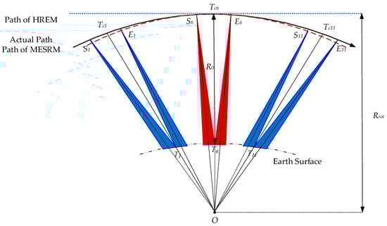
Figure 1.
Geometric model of sliding spotlight mode for space-borne SAR.
The most classic range model utilized in space-borne SAR is the ESRM, in which the straight path approximation is made. The range history described by ESRM can be expressed as
where
where is the azimuth slow time, is the slant range at the Doppler center time, is signal wavelength of the carrier, represents the equivalent radar velocity at the reference azimuth time, represents the equivalent squint angle, is the Doppler centroid frequency, and is the DFMR.
When the synthetic aperture time is not too long, the ESRM can formulate the range history in a concise form. However, as the resolution of the space-borne SAR and the integration time increase, the range deviation between the range model and actual history becomes significant, which is caused by the straight track deviation from the curved orbit. Hence, a more precise range model is needed.
By introducing equivalent radar acceleration into conventional ESRM, the MESRM in [19] can then be expressed as
where
where represents the cubic coefficient, represents the quartic coefficient, denotes the first-order derivation of the DFMR, and is the second-order derivation of DFMR.
Figure 2 shows the phase errors for the ESRM and MESRM as a function of integration time, which indicates the accuracy of these range models. As can be seen, the phase error cause by ESRM increases significantly as the integration time becomes longer. This phenomenon can be explained by Equations (1) and (2), which describe the range history only by the Doppler centroid frequency and the DFMR. As can be seen from (3) and (4), the MESRM not only perfectly describes the actual range history from the first-order to the fourth-order terms but also partially compensates the higher-order terms, leading to a much smaller slant range error. Therefore, the MESRM is more suitable for extremely high azimuth resolution cases, and the accuracy of the MESRM is sufficient for the target at the scene center.
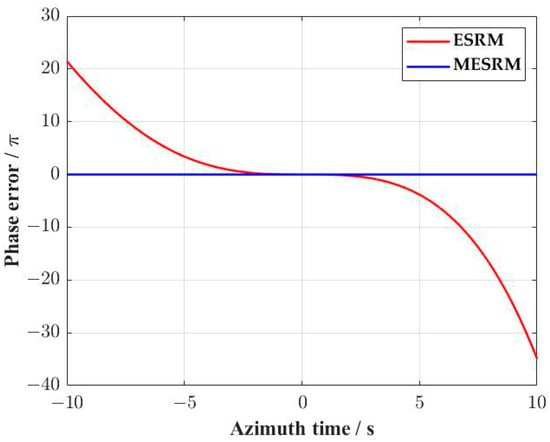
Figure 2.
Phase error caused by range deviation as a function of the integration time in ESRM and MESRM.
Meanwhile, the accuracy of the MESRM for targets with different angles is also analyzed. The range history of eleven targets evenly distributed in the azimuth direction with an interval of 2 km is simulated for different range cells, and the range errors between the simulated range history and the MESRM model for these targets are examined, which are shown in Figure 3. The horizontal axis is the beam-center-time of the stimulated targets, whereas the vertical axis represents the slant range error of the MESRM for these targets and the corresponding Doppler phase error. The synthetic aperture time is set to be 4.65 s, which corresponds to an azimuth resolution of 0.25 m, and the relevant azimuth swath is 20 km. It can be seen from Figure 3 that the accuracy of MESRM deteriorates significantly as the position displacement from the central target increases in azimuth direction, and the phase error even gradually approaches for the targets 10 km away, which indicates that the imaging quality will degrade for marginal targets. Constrained by the maximum phase error of , the azimuth imaging width is approximately limited within 4 km, which is represented by the green solid line in Figure 3. Therefore, the MESRM is not precise enough to match the range history of the points far away from the scene center, i.e., and in Figure 1.
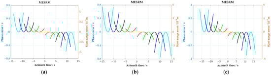
Figure 3.
The slant range error and phase error as a function of azimuth time caused by MESRM. (a–c) represent the errors along azimuth direction in the near, central, and far range cells, respectively. Lines with different colors represent the errors of different targets with a constant interval of 2 km along azimuth direction.
In conclusion, the MESRM can only match the range history for the central point target, but for the azimuth marginal point target, a non-negligible range deviation occurs, which will lead to the severe degradation of the imaging quality.
It can be observed from Figure 3 that the quadratic term is the major component of the slant range error, and the magnitude of this error is approximately proportional to the azimuth displacement of the target relative to the scene center. Therefore, for the targets appearing in the same range cell, there is a quasi-linear mapping relationship between their DFRM errors and the beam-center-times. Essentially, the slant range error for a target is caused by the range deviation between the actual range history during the integration time and a certain segment of the range history corresponding to MESRM, both of which have the same Doppler centroid frequency. The relationship between the slant range error and the DFMR error can be analytically expressed as
where
is the slant range error,
is the DFMR error, represents the absolute value of an element, is the synthetic aperture time, and denotes the beam-center-time of the target positioned at in azimuth direction. In this paper, the variation scope of the DFMR error is limited within 0.0462 Hz/s, which can be obtained by (6). The DFMR error as a function of azimuth time caused by MESRM is displayed in Figure 4, where the red dashed lines are the safe lines corresponding to the maximum phase error of , and the magenta dots identify the eleven targets in the different azimuth positions above. The result demonstrates the quasi-linear mapping relationship between the DFRM errors and the beam-center-times, which can be formulated as
where is the first-order fitting coefficient regarding the azimuth time. The actual DFMR can then be given by
where represents the DFMR of MESRM along different azimuth times and can be given by
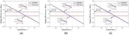
Figure 4.
The DFMR error as a function of azimuth time caused by MESRM. (a–c) represent the DFMR errors at near, central, and far range cells, respectively.
Additionally, the calculation formula of the effective imaging area can be described as
where is the effective imaging time scope, and denotes the velocity of the antenna beam on the ground. As can be seen in Figure 4, the blue solid line indicates that the effective imaging time scope and area are close to 5.8 s and 4 km in the azimuth direction, respectively. The marginal areas will suffer from severe deterioration in imaging quality when the MESRM is utilized.
According to (3) and (5), a Spatial-Variant MSERM (SV-ESRM) is proposed in this paper, which can be formulated as
where .
Compared to the MESRM modeled in Equation (3), a quadratic slant range deviation with respect to azimuth time exists for the marginal targets, which could be observed in Equation (11), and hence, a linear DFRM error correction regarding azimuth time should be introduced to remove the deviation of the DFRM. After the DFRM correction, the phase error for different targets declines significantly, and the maximum phase error is extremely smaller than as shown in Figure 5. The partial magnification result of the phase error indicated by the blue solid line is also displayed in Figure 5, and the maximum phase error is limited within . The SV-ESRM retains a highly precise description of the scene center and also exhibits good performance in modeling the spatial variance. These analyses and simulated results above also highlight the necessity and feasibility of introducing the spatial-variant term.
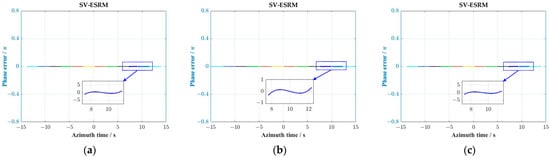
Figure 5.
The phase error as a function of azimuth time caused by MESRM. (a–c) represent the errors along azimuth direction in the near, central, and far range cells, respectively. Lines with different colors represent the errors of different targets with a constant interval of 2 km along azimuth direction.
2.2. The Estabishment of Spatial-Variant Signal Model
According to the previous analyses, the received signal for a point target could be expressed as
where is the scattering coefficient, and represent the antenna pattern functions in the azimuth and range directions, respectively, is the fast time, is the Doppler center time, is the speed of light, is the range phase modulation rate, and is the slant range at the different azimuth time.
The first exponential component in (12) represents the azimuth modulation phase. When neglecting the last term of range history in (11), which is spatially varying with the azimuth position, the residual and spatially variable quadratic azimuth modulation phase will lead to an image defocusing phenomenon in the azimuth profile. To address this problem, a more detailed analysis is given below.
Through the Equations (7) and (8), it can be observed that the small change in the DFMR is formulated by a quasi-linear mapping relationship, which is proportional to the azimuth position of the targets. Naturally, a Doppler phase perturbation method is introduced to eliminate the deviation of the DFMR for MESRM. If the small variation of the DFMR introduced by the Doppler phase perturbation is equal to the deviation of that, precise focusing of the full scene can be realized through one single imaging processing. As shown in earlier analyses, the Doppler phase perturbation function is sufficient to equalize the DFMR along range cells. Considering the first order fitting coefficient , the Doppler phase perturbation function should be expressed as
Then, neglecting the small phase modulation above, the principle of stationary phase (POSP) is used to derive the azimuth-invariant component of the two-dimensional point target spectrum (PTS), which can be obtained as
where and denote the azimuth and range frequency, respectively. is the stationary point and could be derived from the following equation:
The stationary point of the SV-ESRM can be obtained by solving (15), we have
Substituting (16) into (14) leads to
where
3. Imaging Algorithm
Based on the above analyses, an efficient and general imaging algorithm is proposed for HRWS space-borne SAR. The block diagram of the MHCA is shown in Figure 6. Firstly, the novel azimuth preprocessing, which consists of the sub-aperture operation [14,33,34] and the Doppler phase perturbation, is applied to remove the azimuth spectrum aliasing caused by the insufficient Pulse Repetition Frequency (PRF) [33,35] and the azimuth-variance introduced by the last term of (11). Then, the modified focusing processing is adopted to correct the total RCM and compensate the Doppler phase, and the high-precision focusing is subsequently fulfilled within the full wide-swath. The range phase perturbation method is also performed in this step to equalize the range frequency modulation rate across different range cells for further refined focusing. Finally, the residual phase compensation operation is used to remove the image aliasing and residual phase, simultaneously. Details of the proposed imaging algorithm are provided in the following:
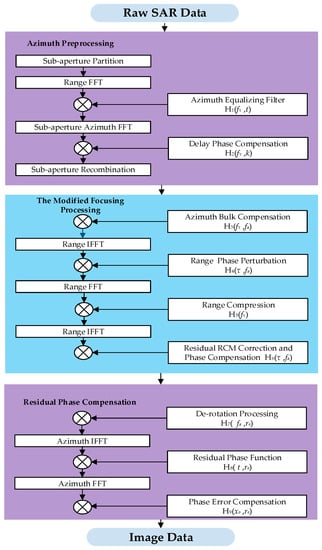
Figure 6.
Block diagram of the MHCA based on the SV-ESRM.
3.1. Azimuth Preprocessing
In the sliding spotlight mode, the azimuth bandwidth is much greater than the PRF. The bandwidth introduced by beam steering occupies a larger proportion. To solve the azimuth aliasing problem of the Doppler spectrum, together with the removing of the azimuth variance of the Doppler parameter, an improved azimuth sub-aperture processing method is adopted here. Compared to traditional processing [36], the novel azimuth equalizing filter adds a Doppler phase perturbation, which is implemented to eliminate the azimuth-variance of the echo signal, while the term “equalize” means adjusting the DFMR to be equal.
The novel azimuth equalizing filter function is given by
where represents the reference slant range, is PRF, is range frequency, is the carrier frequency, is the Doppler center frequency of the th sub-aperture, is the center time of the th sub-aperture, is the rounding down operation, and and denote the size and the azimuth sample number of the sub-aperture, respectively.
Then, the Fast Fourier Transform (FFT) of the sub-aperture along the azimuth direction is performed, and delay phase compensation and sub-aperture recombination are accomplished in the range frequency domain. The two-dimensional spectrum can then be obtained in a discrete form without aliasing in the azimuth direction. The expression of the delay phase compensation function is given by
3.2. The Modified Focusing Processing
After removing the azimuth-variance by the Doppler phase perturbation within the full swath, the modified focusing processing can then be employed to achieve the total RCM correction and phase compensation. Regarding the focusing operation of HRWS space-borne SAR, the total RCM increases significantly, which leads to an apparent decrease in computational efficiency for the conventional hybrid algorithm [20]. Therefore, the focusing processing of the conventional hybrid algorithm is unsatisfied in this case. As a result, the correction of the total RCM in focusing processing is divided into two steps: the bulk RCM correction and subsequently the differential RCM correction, which could keep a balance between the accuracy and the efficiency. The correction of bulk RCM can be achieved by performing the azimuth bulk compensation at the reference range cell. Then, the differential RCM and Doppler phase can be compensated through hybrid correlation processing in the range-Doppler domain. Meanwhile, a range phase perturbation is also implemented to equalize the range frequency modulation rate across different range cells and eliminate the defocusing in range profile for marginal targets. The details of the modified focusing processing are shown as follows.
3.2.1. Azimuth Bulk Compensation
In order to remove the bulk RCM and azimuth phase modulation, the azimuth bulk compensation operation is performed through a complex multiplication with an azimuth reference function at the central range cell. After this operation, the coarse focusing with in the full scene is completed. The reference function is given by
where
where the subscript represents the reference position. is the reference slant range. The slant range corresponding to the central range cell is generally chosen as . Other reference parameters can then be denoted as , , , , and . Next, the Inverse FFT (IFFT) along the range direction is realized. Note that the bulk RCM, azimuth phase modulation, and range-azimuth cross-coupling at the reference slant range are then corrected. The data is then transformed into the range-Doppler domain.
3.2.2. Range Phase Perturbation
On the premise of HRWS space-borne SAR, the residual range-azimuth-coupled spatial variation still exists, which will result in the variance of the range frequency modulation rate across different range cells in the range-Doppler domain. The actual range frequency modulation rate will deviate from that of the transmission signal , which indicates that the length of the hybrid correlation sliding window becomes longer, and the defocusing phenomenon of the range profile may occur for the marginal targets. Thus, the range phase perturbation operation should be introduced to remove the slight deviation in the range frequency modulation rate , which is proportional to the range deviation of the differential RCM from the point at the scene center, and is then introduced by the range phase. Additionally, the length of the sliding window used subsequently will be shortened for the purpose of high efficiency. Figure 7a,b shows the compression result before and after the range phase perturbation, respectively. The range phase perturbation function is given by
where
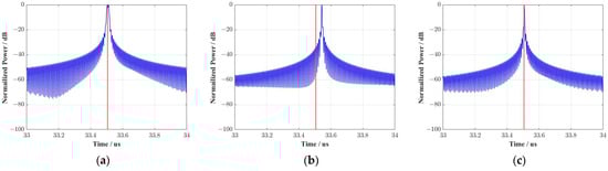
Figure 7.
The results of range phase perturbation processing. (a) Compression result before range phase perturbation. (b) Compression result after range phase perturbation (c) Compensation result of range phase perturbation compensation. The red solid line represents the reference position of range compression.
Substituting with , the equations in (24) can be described as , , and .
After the range phase perturbation operation, the purpose of equalizing the range frequency modulation rate is accomplished. Besides, the range perturbation filter function also brings some side effects, which could be analyzed below.
Expanding the equation (23) based on the Taylor polynomial with respect to , (23) can be written as follows:
where
- The first term : this is a constant component, which varies according to the range position deviation of targets and is negligible when only the amplitude of the image is considered.
- The second term : this is a linear component, which causes a range position shift to the targets. The shift is a quadratic term of time deviation in the range direction and is expressed as
- The third term : the quadratic component equalizes the range frequency modulation rate of different range cells. The range frequency modulation rate is replaced by
- The fourth term : the cubic component is same for all targets, which leads to slightly asymmetric side lobes.
These side effects are compensated by the following processing, which can be incorporated into the residual RCM correction and Doppler phase compensation. The compensation result is revealed in Figure 7c. The red solid line represents the reference position of range compression. Figure 7b,c demonstrates the effectiveness of the range phase perturbation compensation.
3.2.3. Range Compression
FFT along the range direction is achieved for a transformation back to the two-dimensional frequency domain. The range compression for all targets is realized by the range matched filter, which is given by
Next, IFFT along the range direction is performed. The data is then transformed into the range-Doppler domain.
3.2.4. Differential RCM Correction and Doppler Phase Compensation
After azimuth bulk compensation, the differential RCM and Doppler phase still exist in the echo signal. The hybrid correlation processing in the range-Doppler domain is employed to address these problems, and the refined focusing result can be acquired by complex conjugate multiplications in the sliding window between the target echoes and reference functions. The details of the differential RCM correction and Doppler phase compensation are illustrated in the following.
A hybrid correlation sliding window in the range direction is applied, which has the following form:
where represents the length of the sliding window, is the range sample rate, is the differential RCM correction and Doppler phase compensation function, and is the range position shift of the sliding window at the slant range .
where denotes IFFT, and is the complex conjugate, and is given by
3.3. Residual Phase Compensation
The image aliasing in time domain and residual azimuth-variance problems still exist. The azimuth resample operation is adopted to eliminate aliasing and the residual phase. This operation starts with de-rotation processing, which is selected as
where , is the slope of the varying Doppler centroid introduced by beam rotating, and is the hybrid factor, which can be denoted as
where and shown in Figure 1 are the distance from the scene center point and the rotation point O to the radar sensor at the Doppler center time, respectively.
Next, IFFT along the azimuth direction is performed, and the residual phase function, which is expressed in the following, is used to compensated the residual phase.
After the azimuth FFT, the phase error is compensated by , which is given by
where , , , and denote , , and , respectively. The focused SAR image is then described as
4. Simulations and Results
Stimulation results for the point targets are conducted to demonstrate the performance of the MHCA based on the SV-ESRM for HRWS space-borne SAR imaging. The raw SAR data are generated for the point targets using the parameters listed in Table 3, which are laid out on a square area of 20 km 20 km as shown in Figure 8. The distances of different targets along the range and azimuth directions are 10 km and 2.0 km, respectively. The rectangular antenna pattern is assumed in both the range and azimuth directions.
Table 3.
List of simulation parameters.
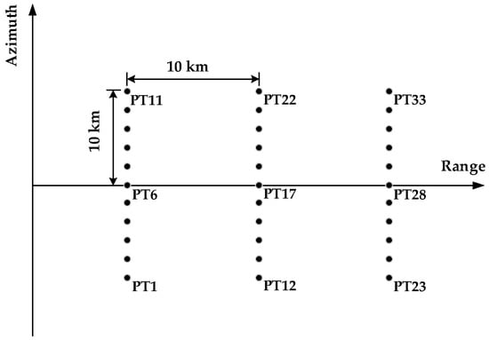
Figure 8.
Ground scene layout of the point targets in the simulation.
4.1. Validation of the Range Phase Perturbation
Due to the spatial variant cross-coupling phase along both the range and azimuth directions in the case of HRWS space-borne SAR, the range frequency modulation rate varies with different range cells, which results in the defocusing phenomenon of the range profile for the point targets at the edge of the swath as can be seen from Figure 7a. Simultaneously, the subsequent problem of a longer sliding window caused by range defocusing will reduce the processing efficiency of the differential RCM correction and Doppler phase compensations. Consequently, the range phase perturbation function is introduced to remove the variation of the range modulation frequency rate across the different range cells and improve the compression result in the range direction. Then, the azimuth bulk compensation within the full wide-swath can be achieved. To illustrate the validation of the range phase perturbation and the consistency with theoretical analyses, the echo signal of the marginal targets is compressed by the range matched filter shown in (30) after the range phase perturbation. Corresponding results are displayed in Figure 7b,c, where Figure 7b represents the compression result before residual effects compensation, and Figure 7c denotes that after residual effects compensation, and the latter result shows that the signal is compressed to the reference position. Up until now, the effectiveness of the range phase perturbation operation has been completely validated. Additionally, the deviation of the stationary phase point introduced by (23) is ignored, which is far smaller than the phase modulation caused by the platform motion in the following processing.
4.2. Validation of the Doppler Phase Perturbation
The point target scene is used in the simulation to illustrate the validation of the Doppler phase perturbation as shown in Figure 8. The preciseness of the conventional range models is analyzed for HRWS space-borne SAR, which indicates their non-adaptability for the full-scene targets in HRWS situations as shown in Figure 2 and Figure 3. Based on the MESRM, the spatial-variant characteristic of the Doppler parameters along the azimuth direction is studied, which reveals that the variation of the DFMR with respect to azimuth time is approximately a quasi-linear mapping relationship observed in Figure 3. Therefore, the Doppler phase perturbation suitable for SV-ESRM is then applied to address this problem. The phase errors of the marginal targets are much smaller than the maximum phase error of as can be seen from Figure 5, which means good compression results can be obtained in the azimuth direction.
The imaging results of eight selected targets (Targets 1, 17–22, 33) corresponding to 0.25 m azimuth resolution are shown to demonstrate the feasibility of the novel hybrid correlation algorithm for HRWS space-borne SAR based on the SV-ESRM. The imaging results of Targets 17–22 are presented in Figure 9 and Figure 10, where (a1–a6) and (b1–b6) represent the focused results of the azimuth profile and the two-dimensional contour before and after azimuth Doppler phase perturbation, respectively. It can then be seen that the central target (Target 17) is well focused, and the azimuth profile is quietly consistent with the theoretical one, whereas the marginal targets (Targets 21 and 22) deviating from the center of the scene suffer from severe degradation in their azimuth profiles. For Targets 18 and 19, slight degradation can also be observed at the same time. For two targets (Targets 1 and 33) positioned at the corner of the scene, the imaging results are presented in Figure 11. It can also be observed that significant defocusing occurs in their azimuth profiles. The aforementioned phenomena are also consistent with the analyses, since the targets positioned at the edge of the scene suffer from the most severe mismatch of the DFMR, which could lead to a distortion of the azimuth profile, including azimuth main-lobe broadening and side-lobe arising. After introducing the Doppler phase perturbation in the proposed MHCA, well-focused azimuth profiles can then be acquired for all targets in the full scene. As a comparison, Figure 10 also shows the imaging results of the JTDRA for the corner points (Targets 1 and 33). As can be seen, the imaging quality of the proposed MHCA is nearly identical with that of the JTDRA. However, the processing efficiency of the MHCA has improved by about 40% in the simulation. The side effects caused by the cubic term of (13) can be ignored during the deviation of the stationary phase point of the signal, which is rather smaller. In order to quantify the imaging processing performance, the evaluation results of the point targets are listed in Table 4, where the ideal Peak Side-Lobe Ratio (PSLR) and the ideal Integrated Side-Lobe Ratio (ISLR) are −13.26 dB and −9.68 dB, respectively. and represent theoretical resolution calculated by the following equation:
where denotes the length of antenna, and is the transmitted bandwidth in the range direction. It is obvious that the deterioration of the Impulse Response Width (IRW) in the range direction is less than 1%, whereas that in the azimuth direction is less than 2%.
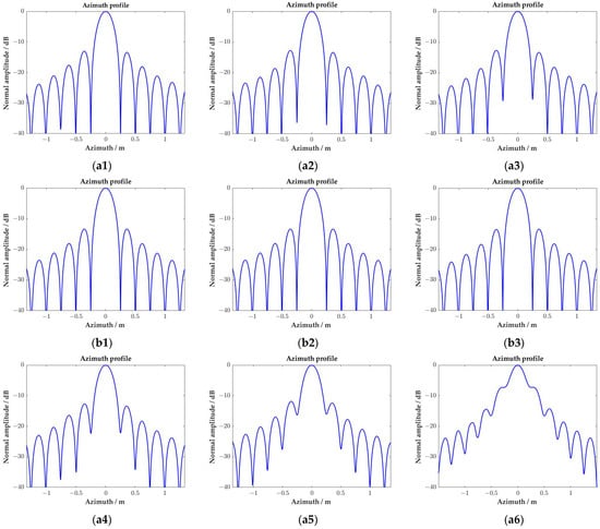
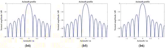
Figure 9.
Evaluated results of azimuth profile for the chosen targets corresponding to 0.25 m azimuth resolution. (a1–a6) The results of Targets 17–22 before the Doppler phase perturbation. (b1–b6) The results of Targets 17–22 after the Doppler phase perturbation. All of the results have been up-sampled by 32× to better illustrate the details.
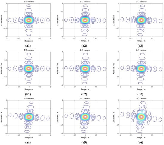
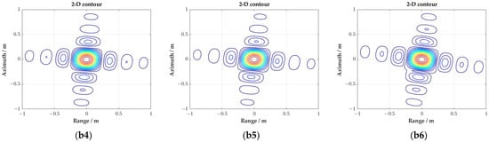
Figure 10.
Evaluated results of azimuth two-dimensional contour for the chosen targets corresponding to 0.25 m azimuth resolution. (a1–a6) The results of Targets 17–22 before the Doppler phase perturbation. (b1–b6) The results of Targets 17–22 after the Doppler phase perturbation. All of the results have been up-sampled by 32× to better illustrate the details.
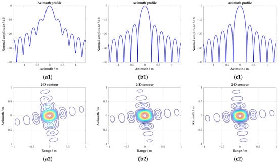
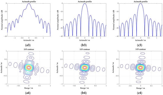
Figure 11.
Evaluated results of azimuth profile and two-dimensional contour for the chosen targets corresponding to 0.25 m azimuth resolution. (a1–c1) The azimuth profile of Target 1 before spatial variance compensation, after Doppler phase perturbation in MHCA, and after azimuth-time resampling in JTDRA, respectively. (a2–c2) The azimuth two-dimensional contour of Target 1 corresponding to (a1–c1). (a3–c3) The azimuth profile of Target 33 before spatial variance compensation, after Doppler phase perturbation in MHCA, and after azimuth-time resampling in JTDRA, respectively. (a4–c4) The azimuth two-dimensional contour of Target 33 corresponding to (a3–c3). All of the results have been up-sampled by 32× to better illustrate the details.
Table 4.
The evaluation results of nine targets.
As shown in Figure 11, an azimuth variant rotation in the range side lobe can be observed in the two-dimensional contour of the targets’ imaging results, which is caused by the variation of the Doppler frequency from the near to far range and the spatial variation of the equivalent squint angle. The range side lobes are distributed along the iso-Doppler line, and the azimuth variant rotation is determined by the Doppler centroid frequency when the target is illuminated by the center of the radar beam.
According to the analyses above, some significant conclusions can be drawn. The imaging results validate the azimuth Doppler phase perturbation and improve the focusing performance, and all the targets in the whole scene are well focused by the advanced algorithm via a batch imaging processing. The evaluation results of the nine targets are present in Table 4.
4.3. Computational Complexity Analysis
The computational complexity of the MHCA and the JTDRA is compared in Table 5. The proposed MHCA requires only complex multiplications, whereas the JTDRA demands two interpolations in the imaging processing. The computational complexities of the MHCA and JDTRA can be summarized by (41) and (42), respectively,
where and are the number of samples in azimuth and range directions, respectively; represents the length of the interpolation kernel, which is chosen as 16 to maintain satisfactory accuracy. Assuming that , the computational complexities of them could be simplified as
Table 5.
Analysis of the computational complexity for different algorithms.
The total computational complexities of the two algorithms with respect to number of samples are shown in Figure 12, which indicates a clear improvement of the proposed MHCA on the computational burden. As is shown in Figure 12b, the computational complexity in dealing with spatial variance dramatically decreases compared to the interpolation operation in JTDRA.
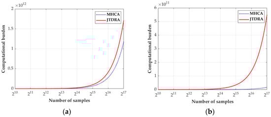
Figure 12.
Comparison of computational complexities for the MHCA and the JTDRA. (a) The computational complexity of the whole algorithm. (b) The computational complexity in dealing with spatial variance.
5. Discussion
The major error of the proposed algorithm is introduced by the Doppler phase perturbation step, which dominates its maximum applicable swath width. In addition to equalizing the DFMR within the range cell, the Doppler phase perturbation step also brings some extra effects. For a target positioned at t0 in the data matrix, The Doppler phase perturbation could be decomposed into four components with different orders:
- The constant component : this term brings a range position shift and causes a phase error , which can be ignored when only the amplitude of the imaging result is considered. Their expressions are given by (45) and (46)
- The linear component : it leads to a small spatially varying Doppler centroid shift to the echo signal , which is a quadratic term as a function of the azimuth time. The linear component will cause a range shift and an azimuth shift to the target position. Moreover, these position shifts should be considered in the geometric calibration
Additionally, the Doppler shift will cause a mismatch on the RCM correction filter, while the corresponding RCM correction error is
The safe line of the RCM error could typically be chosen as
where represents the range resolution. The maximum swath width should satisfy that the RCM correction error for the edge target does not exceed the set safe line.
- The quadratic component : this item is the desired component, which removes the deviation of the DFMR within the same range cell.
- The cubic component : it is a cubic Doppler phase modulation, which is azimuth-invariant and can be identically compensated for all targets, otherwise slight asymmetry of the side lobes will arise for the imaging results. This small phase modulation could be negligible in the derivation of the stationary phase point.
6. Conclusions
For HRWS space-borne SAR working in the sliding spotlight mode, the Spatial-Variant Equivalent Slant Range Model (SV-ESRM), which can precisely describe the range history of the distributed-target echo, is established based on the accuracy analyses of the conventional range models in a larger azimuth swath. Subsequently, the MHCA is proposed on the basis of the SV-ESRM in this paper. A Doppler phase perturbation method incorporated with the sub-aperture operation is performed to remove the DFMR variation of the echo data by the novel azimuth equalizing filter, and the well-focused azimuth results can then be acquired. Simultaneously, a range phase perturbation processing is implemented to equalize the range frequency modulation rate in different range cells and eliminate the defocusing of range profile caused by range-azimuth coupling for the targets at the edge of swath. The modified hybrid correlation method is employed to remove the differential RCM more precisely, which can keep a balance between focusing accuracy and processing efficiency. After the accurate focusing is performed, the residual azimuth variance and imaging aliasing are removed by the residual phase compensation operation. The point target stimulation results demonstrate the accuracy of the SV-ESRM and the effectiveness of the proposed imaging algorithm, which can be applied to HRWS space-borne SAR system.
The spectrum shift introduced by the azimuth equalizing filter discussed in Section 5 increases rapidly for the marginal targets, which limits the maximum applicable scene size of the proposed algorithm. In our future work, methods to eliminate this spectrum shift will be discussed to enhance the applicability of the proposed algorithm.
Author Contributions
Conceptualization, P.W. and J.C.; methodology, P.W. and Y.G.; software, Y.G.; validation, Y.G., Z.M., L.C. and L.Z.; formal analysis, Y.G.; investigation, P.W. and Y.G.; resources, Y.G.; data curation, Y.G.; writing—original draft preparation, Y.G.; writing—review and editing, P.W.; visualization, P.W.; supervision, J.C.; project administration, J.C.; funding acquisition, P.W. All authors have read and agreed to the published version of the manuscript.
Funding
This research was funded by the Innovation Fund Project of Shanghai Aerospace Science and Technology (SAST) under Grant No. SAST2020-038.
Institutional Review Board Statement
Not applicable.
Informed Consent Statement
Not applicable.
Data Availability Statement
The study did not report any data.
Conflicts of Interest
The authors declare no conflict of interest.
Abbreviations
| SAR | Synthetic Aperture Radar |
| HRWS | High-Resolution Wide-Swath |
| ESRM | Equivalent Squint Range Model |
| HREM | Hyperbolic Range Equation Model |
| DRM4 | the fourth-order Doppler Range Model |
| MESRM | Modified Equivalent Squint Range Model |
| SV-ESRM | Spatial-Variant Equivalent Squint Range Model |
| MHCA | Modified Hybrid Correlation Algorithm |
| RCM | Range Cell Migration |
| TSX-NG | TerraSAR-X Next Generation |
| RDA | Range Doppler Algorithm |
| HHCA | High-order Hybrid Correlation Algorithm |
| JTDRA | Joint Time-Doppler Resampling Algorithm |
| FSA | Frequency Scaling Algorithm |
| CSA | Chirp Scaling Algorithm |
| NCS | Nonlinear Chirp Scaling |
| DFMR | Doppler Frequency Modulation Rate |
| POSP | Principle of Stationary Phase |
| PTS | Point Target Spectrum |
| PRF | Pulse Repetition Frequency |
| FFT | Fast Fourier Transform |
| IFFT | Inverse Fast Fourier Transform |
| PSLR | Peak Side-Lobe Ratio |
| ISLR | Integrated Side-Lobe Ratio |
| IRW | Impulse Response Width |
References
- Ciuonzo, D.; Carotenuto, V.; De Maio, A. On Multiple Covariance Equality Testing with Application to SAR Change Detection. IEEE Trans. Signal Process. 2017, 65, 5078–5091. [Google Scholar] [CrossRef]
- Liu, G.; Li, L.; Jiao, L.; Dong, Y.; Li, X. Stacked Fisher autoencoder for SAR change detection. Pattern Recognit. 2019, 96, 106971. [Google Scholar] [CrossRef]
- Yang, W.; Chen, J.; Liu, W.; Wang, P. Moving Target Azimuth Velocity Estimation for the MASA Mode Based on Sequential SAR Images. IEEE J. Sel. Top. Appl. Earth Observ. Remote Sens. 2017, 10, 2780–2790. [Google Scholar] [CrossRef] [Green Version]
- Jung, H.; Lu, Z.; Shepherd, A.; Wright, T. Simulation of the SuperSAR Multi-Azimuth Synthetic Aperture Radar Imaging System for Precise Measurement of Three-Dimensional Earth Surface Displacement. IEEE Trans. Geosci. Remote Sens. 2015, 53, 6196–6206. [Google Scholar] [CrossRef]
- Townsend, W. An initial assessment of the performance achieved by the Seasat-1 radar altimeter. IEEE J. Ocean. Eng. 1980, 5, 80–92. [Google Scholar] [CrossRef] [Green Version]
- Moreira, A.; Prats-Iraola, P.; Younis, M.; Krieger, G.; Hajnsek, I.; Papathanassiou, K.P. A tutorial on synthetic aperture radar. IEEE Geosci. Remote Sens. Mag. 2013, 1, 6–43. [Google Scholar] [CrossRef] [Green Version]
- Villano, M.; Krieger, G.; Moreira, A. Staggered SAR: High-Resolution Wide-Swath Imaging by Continuous PRI Variation. IEEE Trans. Geosci. Remote Sens. 2014, 52, 4462–4479. [Google Scholar] [CrossRef]
- Cerutti-Maori, D.; Sikaneta, I.; Klare, J.; Gierull, C.H. MIMO SAR Processing for Multichannel High-Resolution Wide-Swath Radars. IEEE Trans. Geosci. Remote Sens. 2014, 52, 5034–5055. [Google Scholar] [CrossRef]
- De Almeida, F.Q.; Younis, M.; Krieger, G.; Moreira, A. A New Slow PRI Variation Scheme for Multichannel SAR High-Resolution Wide-Swath Imaging. In Proceedings of the 2018 IEEE International Geoscience and Remote Sensing Symposium, Valencia, Spain, 22–27 July 2018; pp. 3655–3658. [Google Scholar]
- De Almeida, F.Q.; Younis, M.; Prats-Iraola, P.; Rodriguez-Cassola, M.; Krieger, G.; Moreira, A. Slow Pulse Repetition Interval Variation for High-Resolution Wide-Swath SAR Imaging. IEEE Trans. Geosci. Remote Sens. 2021, 59, 5665–5686. [Google Scholar] [CrossRef]
- Janoth, J.; Gantert, S.; Koppe, W.; Kaptein, A.; Fischer, C. TerraSAR-X2—Mission overview. In Proceedings of the 2012 IEEE International Geoscience and Remote Sensing Symposium, Munich, Germany, 22–27 July 2012; pp. 217–220. [Google Scholar]
- Janoth, J.; Gantert, S.; Schrage, T.; Kaptein, A. Terrasar next generation—Mission capabilities. In Proceedings of the 2013 IEEE International Geoscience and Remote Sensing Symposium-IGARSS, Melbourne, VIC, Australia, 21–26 July 2013; pp. 2297–2300. [Google Scholar]
- Janoth, J.; Jochum, M.; Petrat, L.; Knigge, T. High Resolution wide Swath—The Next Generation X-Band Mission. In Proceedings of the IGARSS 2019—2019 IEEE International Geoscience and Remote Sensing Symposium, Yokohama, Japan, 28 July–2 August 2019; pp. 3535–3537. [Google Scholar]
- Mittermayer, J.; Moreira, A.; Loffeld, O. Spotlight SAR data processing using the frequency scaling algorithm. IEEE Trans. Geosci. Remote Sens. 1999, 37, 2198–2214. [Google Scholar] [CrossRef]
- Sun, X.; Yeo, T.S.; Zhang, C.; Lu, Y.; Kooi, P.S. Time-varying step-transform algorithm for high squint SAR imaging. IEEE Trans. Geosci. Remote Sens. 1999, 37, 2668–2677. [Google Scholar]
- Eldhuset, K. A new fourth-order processing algorithm for spaceborne SAR. IEEE Trans. Aerosp. Electron. Syst. 1998, 34, 824–835. [Google Scholar] [CrossRef] [Green Version]
- Eldhuset, K. Ultra high resolution spaceborne SAR processing. IEEE Trans. Aerosp. Electron. Syst. 2004, 40, 370–378. [Google Scholar] [CrossRef]
- Eldhuset, K. Spaceborne Bistatic SAR Processing Using the EETF4 Algorithm. IEEE Geosci. Remote Sens. Lett. 2009, 6, 194–198. [Google Scholar] [CrossRef]
- Wang, P.; Liu, W.; Chen, J.; Niu, M.; Yang, W. A High-Order Imaging Algorithm for High-Resolution Spaceborne SAR Based on a Modified Equivalent Squint Range Model. IEEE Trans. Geosci. Remote Sens. 2015, 53, 1225–1235. [Google Scholar] [CrossRef] [Green Version]
- Wu, C.; Liu, K.Y.; Jin, M. Modeling and a Correlation Algorithm for Spaceborne SAR Signals. IEEE Trans. Aerosp. Electron. Syst. 1982, 18, 563–575. [Google Scholar] [CrossRef]
- Bamler, R. A comparison of range-Doppler and wavenumber domain SAR focusing algorithms. IEEE Trans. Geosci. Remote Sens. 1992, 30, 706–713. [Google Scholar] [CrossRef]
- Li, Y.; Zhang, Z.; Xing, M.; Bao, Z. Bistatic Spotlight SAR Processing Using the Frequency-Scaling Algorithm. IEEE Geosci. Remote Sens. Lett. 2008, 5, 48–52. [Google Scholar] [CrossRef]
- Raney, R.K.; Runge, H.; Bamler, R.; Cumming, I.G.; Wong, F.H. Precision SAR processing using chirp scaling. IEEE Trans. Geosci. Remote Sens. 1994, 32, 786–799. [Google Scholar] [CrossRef]
- Moreira, A.; Huang, Y. Airborne SAR processing of highly squinted data using a chirp scaling approach with integrated motion compensation. IEEE Trans. Geosci. Remote Sens. 1994, 32, 1029–1040. [Google Scholar] [CrossRef]
- Moreira, A.; Mittermayer, J.; Scheiber, R. Extended chirp scaling algorithm for air- and spaceborne SAR data processing in stripmap and ScanSAR imaging modes. IEEE Trans. Geosci. Remote Sens. 1996, 34, 1123–1136. [Google Scholar] [CrossRef]
- Liu, W.; Sun, G.; Xia, X.; Chen, J.; Guo, L.; Xing, M. A Modified CSA Based on Joint Time-Doppler Resampling for MEO SAR Stripmap Mode. IEEE Trans. Geosci. Remote Sens. 2018, 56, 3573–3586. [Google Scholar] [CrossRef]
- Wong, F.H.; Cumming, I.G.; Neo, Y.L. Focusing Bistatic SAR Data Using the Nonlinear Chirp Scaling Algorithm. IEEE Trans. Geosci. Remote Sens. 2008, 46, 2493–2505. [Google Scholar] [CrossRef] [Green Version]
- Sun, G.; Xing, M.; Wang, Y.; Yang, J.; Bao, Z. A 2-D Space-Variant Chirp Scaling Algorithm Based on the RCM Equalization and Subband Synthesis to Process Geosynchronous SAR Data. IEEE Trans. Geosci. Remote Sens. 2014, 52, 4868–4880. [Google Scholar]
- Huang, L.; Qiu, X.; Hu, D.; Han, B.; Ding, C. Medium-Earth-Orbit SAR Focusing Using Range Doppler Algorithm with Integrated Two-Step Azimuth Perturbation IEEE Geosci. Remote Sens. Lett. 2015, 12, 626–630. [Google Scholar] [CrossRef]
- Davidson, G.W.; Cumming, I.G.; Ito, M.R. A chirp scaling approach for processing squint mode SAR data. IEEE Trans. Aerosp. Electron. Syst. 1996, 32, 121–133. [Google Scholar] [CrossRef]
- Huang, L.; Qiu, X.; Hu, D.; Ding, C. Focusing of Medium-Earth-Orbit SAR with Advanced Nonlinear Chirp Scaling Algorithm. IEEE Trans. Geosci. Remote Sens. 2011, 49, 500–508. [Google Scholar] [CrossRef]
- Wang, P.B.; Liu, W.; Chen, J.; Yang, W.; Han, Y. Higher order nonlinear chirp scaling algorithm for medium Earth orbit synthetic aperture radar. J. Appl. Remote Sens. 2015, 9, 096084. [Google Scholar] [CrossRef] [Green Version]
- Prats, P.; Scheiber, R.; Mittermayer, J.; Meta, A.; Moreira, A. Processing of Sliding Spotlight and TOPS SAR Data Using Baseband Azimuth Scaling. IEEE Trans. Geosci. Remote Sens. 2010, 48, 770–780. [Google Scholar] [CrossRef] [Green Version]
- Prats, P.; Scheiber, R.; Mittermayer, J.; Meta, A.; Moreira, A.; Sanz-Marcos, J. A SAR processing algorithm for TOPS imaging mode based on extended chirp scaling. IEEE Int. Geosci. Remote Sens. Symp. 2007, 148–151. [Google Scholar]
- An, D.; Huang, X.; Jin, T.; Zhou, Z. Extended Two-Step Focusing Approach for Squinted Spotlight SAR Imaging IEEE Trans. Geosci. Remote Sens. 2012, 50, 2889–2900. [Google Scholar] [CrossRef]
- Luo, Y.; Zhao, B.; Han, X.; Wang, R.; Song, H.; Deng, Y. A Novel High-Order Range Model and Imaging Approach for High-Resolution LEO SAR. IEEE Trans. Geosci. Remote Sens. 2014, 52, 3473–3485. [Google Scholar] [CrossRef]
Publisher’s Note: MDPI stays neutral with regard to jurisdictional claims in published maps and institutional affiliations. |
© 2022 by the authors. Licensee MDPI, Basel, Switzerland. This article is an open access article distributed under the terms and conditions of the Creative Commons Attribution (CC BY) license (https://creativecommons.org/licenses/by/4.0/).