Abstract
Due to the strong speckle noise caused by the seabed reverberation which makes it difficult to extract discriminating and noiseless features of a target, recognition and classification of underwater targets using side-scan sonar (SSS) images is a big challenge. Moreover, unlike classification of optical images which can use a large dataset to train the classifier, classification of SSS images usually has to exploit a very small dataset for training, which may cause classifier overfitting. Compared with traditional feature extraction methods using descriptors—such as Haar, SIFT, and LBP—deep learning-based methods are more powerful in capturing discriminating features. After training on a large optical dataset, e.g., ImageNet, direct fine-tuning method brings improvement to the sonar image classification using a small-size SSS image dataset. However, due to the different statistical characteristics between optical images and sonar images, transfer learning methods—e.g., fine-tuning—lack cross-domain adaptability, and therefore cannot achieve very satisfactory results. In this paper, a multi-domain collaborative transfer learning (MDCTL) method with multi-scale repeated attention mechanism (MSRAM) is proposed for improving the accuracy of underwater sonar image classification. In the MDCTL method, low-level characteristic similarity between SSS images and synthetic aperture radar (SAR) images, and high-level representation similarity between SSS images and optical images are used together to enhance the feature extraction ability of the deep learning model. Using different characteristics of multi-domain data to efficiently capture useful features for the sonar image classification, MDCTL offers a new way for transfer learning. MSRAM is used to effectively combine multi-scale features to make the proposed model pay more attention to the shape details of the target excluding the noise. Experimental results of classification show that, in using multi-domain data sets, the proposed method is more stable with an overall accuracy of 99.21%, bringing an improvement of 4.54% compared with the fine-tuned VGG19. Results given by diverse visualization methods also demonstrate that the method is more powerful in feature representation by using the MDCTL and MSRAM.
1. Introduction
As a main detection approach for many underwater tasks—such as maritime emergency rescue, wreckage salvage, and military defense—side-scan sonar (SSS) can quickly search sizeable areas and obtain continuous two-dimensional images of the marine environment, even in low-visibility water [1,2]. The underwater search procedure usually adopted by engineers is to first scan the target sea area with sonar, then export the image after a global scan, and finally judge whether there is a target according to the experience of the sonar operator [3]. However, manual judgement is of low efficiency, time-consuming, resource intensive, and overly reliant on experience. With the development of equipment such as unmanned ships and autonomous underwater vehicles (AUVs) [4], how to identify the sunken target in SSS images accurately, quickly, and automatically becomes increasingly important. In order to achieve automatic operation of AUVs, researchers have done a great deal of work on automatic target classification (ATC) in SSS images [5,6,7,8,9].
Seabed reverberation and the complex underwater environment cause various noises in sonar images, such as speckle noise, Gaussian noise, and impulse noise—the most prominent one of which is speckle noise [10]. Speckle noise [11], represented by the random particles of brighter and darker pixels in sonar images, will lead to the loss of image details, contrast reduction, and edge blur, and therefore it makes the feature extraction of the targets in sonar images more difficult. Traditional underwater sonar image classification methods, developed from the optical image classification methods, usually include noise reduction preprocessing, feature extraction, feature classification, and other steps [12,13]. The key module of sonar image classification is feature extraction, which usually have to be noise robust. Traditional feature extraction methods can be divided into local feature descriptors and model-based methods. Local feature descriptors, without prior knowledge, can extract shallow visual features, such as the Haar feature [14], Haar-like and the local binary pattern (LBP) features [15], scale invariant feature transform (SIT) features [16,17], and oriented FAST and rotated BRIEF (ORB) features [18]. With the use of prior knowledge or driven data, model-based methods have also been proposed for feature extraction, which needs great consistency and similarities between testing and training datasets. Myers [19] combined the information from both highlight regions and shadow regions with multi-view templates to improve the classification accuracy. Hausdorff distance from the synthetic shadows to the real object shadow was combined with highlight and scale information to produce a membership function, and then the objects were classified using both mono-view and multi-view analysis with the help of Dempster–Shafer information theory [20].
The extracted features are used to train classifiers, such as hidden Markov model [21], k-nearest neighbor model [22], support vector machine (SVM) [23], and other classifiers to realize underwater target recognition. Çelebi [24] used Markov Random Fields to detect potential mines in the SSS images after compensating for illumination variations. The effectiveness and generality of the trained classifiers are limited due to the poor quality of noisy sonar images and the specificity of artificial feature templates. Moreover, when the recognition task or the corresponding environment changes, the feature templates need to be adjusted and the classification models may also need to be redesigned, which is time-consuming and inconvenient.
In recent years, with the tremendous increase in computational power, convolutional neural networks (CNNs), as a representative method for deep learning, have been widely used in computer vision and natural language. Unlike artificially designed features, CNNs, inspired by the human visual system, can learn features at different levels of abstraction, and therefore are more applicable to image understanding, especially in the field of image recognition and classification [25,26]. The ATC of SSS images using deep learning (DL) methods has become a new trend. Over the past few years, the use of CNNs in SSS image classification has proved to be more effective than traditional image processing methods [3,8,9,27,28,29]. Luo [9] proposed a shallow CNN for classifying seabed which outperformed deep CNN in classification accuracy and speed. In [3], Ye tried to apply the pretrained VGG11 and ResNet18 to classify underwater targets in SSS images and presented the pre-processing method for the training samples which is meaningful in transfer learning. Huo [8] demonstrated that semisynthetic data can benefit fine-tuning a lot and the pretrained VGG19 after fine-tuning had better performance than the models trained from scratch. Qin [27] introduced generative adversarial networks (GANs) to enhance the small size dataset to improve the accuracy of sediment classification. Gerg [28] proposed a structural prior driven regularized deep learning method which outperformed other methods for synthetic aperture sonar image classification. Zhang [29] used automatic deep learning (AutoDL) in classification of sonar images, and their model achieved excellent accuracy at 99.0% after 2.9 h of training. However, the following problems must be overcome when using the DL methods in SSS image classification.
One problem is that, owing to the lack of SSS images, the DL-based models cannot be fully trained, which can cause over fitting—i.e., the model has a poor generalization ability. In order to tackle the challenge of lacking datasets, data enhancement and transfer learning methods have been adopted to improve the generalization ability of the DL-based models.
Data enhancement methods can be categorized according to the types of data synthesis as follows.
- Data transformation rules, such as flipping, rotating, cropping, distorting, scaling, and adding noise, are used on the existing images to enhance data. Inoue [30] used two randomly selected images from the training set and processed them by basic data enhancement operations. Then, a new sample can be formed by averaging two processed images in pixel with one of the original sample labels set as the new label.
- Multiple samples are used to generate similar pseudo samples. The input optical image is preprocessed and combined with sonar image features to create semi synthetic training data to enhance the dataset [8,31]. The method of style transferring with a pre-trained CNN was adopted to generate pseudo SSS images, which can be added to the training set, finally achieving a similar improvement compared with the former method [32]. By changing the upsampling method of style transfer [33], the noise ratio can be changed by manually adjusting parameters, and the generated pseudo SSS images are more related to the real SSS images.
- The randomly generated samples with consistent distribution of the training dataset are created by the generative adversarial networks (GAN), which are trained to learn an image-translation from low-complexity ray-traced images to real sonar images [27,34]. Sung [35] et al. introduced a method of GAN to translate actual sonar images into simulator-like sonar images to generate a great deal of template images.
Meanwhile, transfer learning [36] can also efficiently relieve the pressure of the lack of datasets. Pre-trained CNNs—e.g., the neural networks pre-trained by ImageNet dataset—are usually used [37,38,39], which can somewhat improve the performance of the model when trained with a small-size dataset.
In the method of style transfer, the final synthesized images have the noise from sonar images and the target contour features from optical image. Therefore, the model trained with synthesized images can have a better ability of extracting features from noise background and identifying contour features simultaneously. Therefore, we try to utilize different features of multi-domain images instead of synthesizing data to guide the training of classification model on a limited SSS dataset.
Another problem is that the complex characteristics of SSS images—such as blurred edges, strong noise, and various shapes of targets—bring great difficulties in extracting useful features in SSS images. Traditional image preprocessing methods may lead to the loss of detail information, while the pre-trained models based on a large optical dataset are unable to entirely match the SSS image features. Therefore, it is also important to make the model focus on useful features and extract all available features as much as possible.
Inspired by the inter-domain transfer learning methods [40,41] and the neural network architecture proposed by the Google company [42], the main contributions of the paper are as follows:
- An automatic side-scan sonar image classification method is proposed, which combines the multi-domain collaborative transfer learning (MDCTL) with the multi-scale repeated attention mechanism (MSRAM). The proposed MDCTL method transfers the parameters of low-level feature extraction layers learned from the SAR images and the high-level feature representation layers learned from the optical images, respectively, which gives a new way of transfer learning.
- By combining the channel attention mechanism (CAM) and the spatial attention mechanism (SAM) [43,44], the MSRAM makes the model do better in extracting and focusing on features of the target, and therefore more key features can be used for classification, which brings the model higher classification accuracy, as well as stability.
- The proposed MDCTL method has been tested on a new SSS dataset, which adds 115 more side-scan sonar images to the SeabedObjects-KLSG dataset. The new SSS dataset is now available at https://github.com/HHUCzCz/-SeabedObjects-KLSG--II (accessed on 16 November 2021). Feature response maps and class activation heatmaps are used to demonstrate the effect of the proposed MDCTL method with MSRAM.
The remainder of this paper is organized as follows. Section 2 details the proposed SSS classification method with MDCTL and MSRAM. Section 3 verifies the method proposed by the experiments. In Section 4, the advantages and limitations of this method are discussed. Finally, some conclusions are given in Section 5.
2. Materials and Methods
2.1. Multi-Domain Collaborative Transfer Learning
2.1.1. Fine-Tuning
Typical CNNs have a deep network structure with a huge number of weight parameters to be optimized. Therefore, it needs a great number of training samples to determine all the parameters. For instance, the ImageNet dataset of optical images contains over 1,000,000 labeled training samples. However, for the sonar image classification task which usually relies on a small dataset, the CNN cannot achieve ideal results because the network is hard to train sufficiently from scratch. Transfer learning, which transfers knowledge from the source domain to the target domain, can help to improve the learning ability of a model using only a limited data in the target domain. Transfer learning methods can be categorized as instance-based, parameter-based, adversarial-based, and mapping-based methods [36].
With the application of deep learning in those domains without a large number of training samples, transfer learning has gradually become a popular solution to the problem of inability to apply deep learning. There are two major transfer learning scenarios. In scenario one, an existing network such as a CNN is used as a fixed feature extractor. First, after replacing the last layer or layers in the network, bottleneck features are extracted from the rest network with the inputted image passing through. Then the classification is done in the feature space where classes can be easily discriminated with the bottleneck features. The commonly used classifiers are the Softmax and SVM classifiers [45], which have to learn from the limited training data in the target domain. In scenario two, a method called fine-tuning first replaces the classifier with a new CNN classifier to match the classes of the new dataset and then retrains the whole network or a subset of the network layers using the new dataset based on a pre-trained model [37,38,39]. These two scenarios are both parameter-based. In the scenario one, the parameters are frozen, and the pre-trained network is only used as a feature extractor, and finally the classifier is used to map the extracted features. When the parameters are frozen, the network is unable to learn new knowledge in a new task. Therefore, if the dataset for the new classification task is not strongly related to the dataset used for pre-training, it is very necessary to unlock and retrain some or all of the parameters in the task domain. Fine-tuning is more suitable for learning new knowledge from similar image datasets to perform the classification task.
As shown in Figure 1, after training on a large-scale optical image dataset—e.g., ImageNet—the model can be quickly applied to classification of over 1000 common target categories. However, for underwater SSS images classification, the model pre-trained on optical images is unable to achieve satisfactory results because sonar images and optical images are quite different, and the size of sonar image dataset used for training is very small.
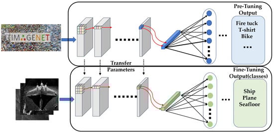
Figure 1.
The architecture of fine-tuning the pre-trained CNN model initialized with the weights trained by ImageNet.
2.1.2. Transfer Learning from Multi-Domain
Considering that methods of transfer learning are unable to achieve optimal results due to the small size of training samples in some special applications, some scholars have focused on the methods of sample generation for enhancing the dataset [8,27,31,32,33,34]. For instance, in the data enhancement method for sonar images, the pseudo-sample synthesis model takes a conventional optical image and SSS images as inputs to generate a pseudo-SSS image with the content of the optical image but with the characteristics of the SSS image. The pseudo-SSS images can improve the model’s ability of feature extraction and feature representation during training. However, due to the complex noise of SSS images, the class imbalance in the dataset, and the different poses of the targets, data enhancement methods using pseudo-samples can only play a limited role in SSS image classification tasks.
Therefore, we try to make the DL-based models learn a powerful feature representation directly from both real SAR and optical datasets instead of from synthetic samples. After training on the SAR dataset with a pre-trained VGG19 network, the convolutional layers close to the input layer can improve the ability of extracting the low-level edge features from the noisy background of the target in SSS images which usually have noise statistical characteristics similar to SAR images. Meanwhile, the selected optical dataset has the same target categories as the SSS dataset—i.e., ships, airplanes, and seabed—and therefore the optical images have similar shape characteristics to the same target category in SSS images. After training a pre-trained VGG19 network on the optical dataset, the several fully-connected (FC) layers close to the output layer enhance the ability to map the high-level feature vector to the semantic space of the sample categories. Finally, parameters of the two models learned from different domains are transferred to the classification model of the SSS image to obtain better low-level and high-level feature extraction and representation capabilities.
Let be the SAR image dataset (feature-source domain), be the optical image dataset (content-source domain), and be the SSS image dataset (target domain), where , and ti respectively denote the categories of labels in SAR image dataset, optical image dataset and SSS image dataset. It should be noted that is equal to because there are the same target categories in both optical image dataset and SSS image dataset. Learning the similar shape information in the source domain can improve the model’s ability to map the shape features learned to the target domain.
As shown in Figure 2, in source domains, the classification models for SAR and optical images cannot be used for classification of SSS images directly, therefore it is necessary to transfer some useful parameters to the target model. It should be noted that SAR and optical images are used as the auxiliary tasks. The loss function of an auxiliary task is defined as
where M represents the number of source domain samples used in the training, represents the convolution and pooling layers, represents the FC layers of the network model, represents the i-th sample used in the source domain training, and represents the label corresponding to the i-th sample.
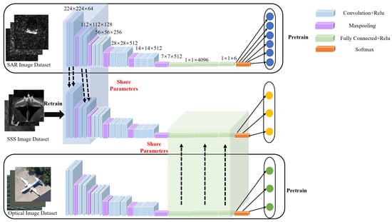
Figure 2.
Architecture diagram of transfer learning from multi-domain.
Classifying SSS images in the target domain is the main task, and its loss function is defined as . Let N represent the number of target domain samples used in the training, the loss function is defined as
The total loss function is defined as
If the size of the sample dataset in the source domain is too large compared to that in the target domain, parameter transfer will result in overfitting, which will have a negative impact on the target domain task, and therefore the constraint coefficient ε is introduced to prevent overlearning in the source domain.
2.2. Backbone Network-VGG19
The VGG19 network is a deep convolutional neural network structure jointly developed by the Computer Vision Laboratory of Oxford University and the group of Google DeepMind, which is used for classification and positioning of 1000 categories of images in ImageNet. As shown in Figure 3, VGG19 has a simple network structure, which includes 5 convolutional blocks and 3 full connection blocks. Each convolution block uses a continuous 3 × 3 convolution kernel to replace the larger convolution kernel, which reduces the number of parameters while expanding the receptive field. Therefore, VGG19 is a good feature extractor, and the layer-by-layer structure is very convenient for parameter transfer learning, so VGG19 is selected as the backbone network in this paper. In addition, the generalization ability of the pre-trained VGG19 has been proved to be very powerful, due to its good performance on different data sets after transfer learning.
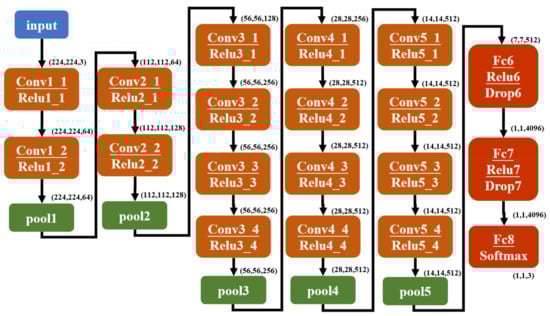
Figure 3.
Detailed architecture diagram of the VGG19 network.
In this paper, we will fine-tune the VGG19 trained on the ImageNet dataset, and replace the last full connected layer and Softmax layer to match the number of categories of samples in the target domain. After re-training with the SSS images dataset, the model obtained an overall accuracy of 94.5% in the classification task, which is used as the baseline in this paper.
2.3. Attention Mechanism
Inspired by the attention mechanism in human perception [46], there have been attempts [43,44] to incorporate attention processing into CNNs to make them exploit a sequence of partial glimpses and selectively focus on salient parts in order to better capture visual structure.
2.3.1. Channel Attention Module
The channel attention module is used to explore the relationship of feature maps between different channels. Each channel itself acts as a feature detector, but has different impact on feature extraction. With the channel attention module, the model can learn which channel output features should be paid more attention.
Traditional algorithms such as squeeze and excitation network (SENet) [47] and bottleneck attention module (BAM) [44] use average pooling in the channel attention branch to compress the spatial dimensions, which fails to fully extract detailed features; CBAM [43] sums the average pooling result and the maximum pooling result directly, which is not yet enough. Therefore, in order to fully preserve the background and detailed information, this paper contacts the two pooling results, as shown in Figure 4a.
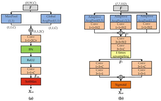
Figure 4.
Improved attention modules: (a) Improved CAM; (b) Improved SAM.
Given that the dimensions of the input feature maps F are (H, W, C), weights need to be assigned to each feature map in X in dimension C based on its importance. The process is that the initial feature is firstly spatially compressed and mapped from space (H, W, C) to space (1, 1, C) to remove the interference of spatial position information; and the global average pooling and global maximum pooling methods are then used, and the pooling results are contacted to obtain the feature maps with dimensions (B, 1, 1, 2C). As the initial input feature maps have C channels, two 1 × 1 convolution kernels are needed to reduce the number of channels to further extract the channel features. Let r represent the channel compression rate, with r = 16 used in this experiment. The above process can be expressed as
where BN is the normalization layer; ReLU is the activation function; represents the channel characteristic matrix; and the corresponding weight matrix will be obtained after passing through the softmax layer.
2.3.2. Spatial Attention Module
Spatial attention helps to remove the interference information of the image background. For instance, CBAM uses the pooling operation to compress the channel in the spatial branch, and BAM uses the serial convolution and dilated convolution to compress the channel. In order to get richer feature information, this paper uses parallel convolution structures of different sizes when compressing channels. To get diversified feature information, two convolutional kernel sizes of 1 × 1 and 3 × 3 are used respectively, and the 3 × 3 size convolutional kernel is split into 1 × 3 and 3 × 1 size convolutional kernel in different order, which can effectively reduce the amount of calculation.
In this paper, the spatial attention mechanism is implanted into the back-end of the network, and the high-level feature is pooled to enrich the global semantic information. Then the high-level pooled feature map is sampled to the scale of each low-level feature (k = 2, 4, 8) and converted into the attention maps. The specific implementation process is summarized as Equation (6). Firstly, two branch convolutional structure with convolution kernel sizes of respectively 1 × 3, 3 × 1 and 3 × 1, 1 × 3 are constructed to extract the semantic information of unsampled features in different directions and orders. Finally, the features got from the two branches are added together and be mapped into the [0,1] interval to get the attention map by the sigmoid activation function. The above process can be expressed as
where F represents feature map outputted from the final convolution block.
2.3.3. Multi-Scale Repeated Attention Module
Due to the large number of convolutional kernels in the convolutional layers of the backbone network, the output of each convolution kernel is quite different when the input is the same. The channel attention mechanism is equivalent to adding a multiplicative weight to the output feature of each convolution kernel, which increases the importance of the convolutional kernel with strong feature extraction ability in the convolutional layer. Therefore, the channel attention module is used to make a model pay more attention to the useful edge information in the low-level feature response map, which can improve the ability of feature extraction. The spatial attention module focuses on the importance of different positions on the feature map, i.e., the positions of useful semantic feature in the high-level feature map. However, the low-level feature map contains not only edge information but also a lot of unimportant background information, which is easy to interfere with the position information of the target. In order to help the network to focus on target and nearby useful information, the attention map of the back-end spatial attention module is upsampled for the front-end low-level feature extraction module to know where the key feature is.
As is shown in Figure 5, the process details are as follows: firstly, the feature map F of a certain layer passes through the channel attention branch to get the channel weight matrix , while the spatial weight matrix can be obtained by upsampling the high-level spatial attention feature map. Secondly, by multiplying F with , the network can assign weights to the input of different kernels according to importance, and the feature maps from relevant kernels have higher weight value. Thirdly, the result is multiplied by , so that the network can learn the position information of the important area of each feature map to remove the interference of irrelevant background. In this process, the results of the two attention branches are successively applied to the input feature matrix, which reflects the repeated operation of the attention mechanism in this paper. Finally, the attention result is combined with the input feature F as residual feature reuse. The process can be expressed as
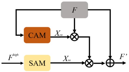
Figure 5.
Architecture diagram of proposed repeated attention mechanism.
2.4. Proposed Network
In this paper, based on a VGG19 classification model trained on SAR and optical image datasets, the method of parameter transfer learning is used to achieve two different aspects of knowledge from multiple source domains, which cooperatively work for SSS image classification task. Meanwhile, SAM will provide the key position information for multi-scale CAMs to further improve feature extraction. The detailed process is as follows.
- Multi-domain pre-training: Using the VGG19 pre-trained on ImageNet dataset, the corresponding classification models are trained on SAR images and optical images respectively;
- Parameter transfer: The VGG19 model, pre-trained on the ImageNet dataset, is set as the backbone. The first two convolutional blocks of the SAR image classification network are first transferred as a new feature extraction branch; the last three convolutional layers of the optical image classification network will then replace the corresponding layers of the SSS image classification network. The transferred parameters will be unfrozen and retrained to fit the SSS image classification task in the target domain;
- Adding multi-scale repeated attention mechanism: SAM is placed at the back end of the network to obtain the spatial attention map through the feature map output from the last convolution layer. Then, the spatial attention map will be upsampled into different scales to multiply with the channel weight matrix obtained from CAM.
As shown in Figure 6, by using transfer learning, the classification model in target domain can learn from multiple source domain datasets in different modules, i.e., the feature extraction module trained on the SAR image dataset and the feature representation module trained on the optical image dataset.
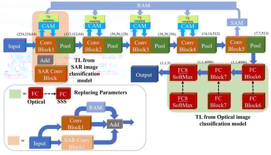
Figure 6.
Architecture diagram of proposed MDCTL-MSRAM network.
Since the statistical features of SAR images are similar to those of SSS images, the convolutional layers close to the input layer are more capable of extracting target edge features and detailed information from noisy images. Therefore, we select part of the convolutional layers as an additional feature extractor, and unfreeze the parameters to make it retrainable to the target task. Likewise, as the selected optical dataset has the same categories as the SSS image dataset, the fully connected layers near the output pay more attention to the contour features corresponding to these categories; therefore, we replace all the fully connected layers and unfreeze the parameters to retrain them. The method of transfer learning from multi-domains is adopted to exclude useless noise and make model focus on useful features.
However, traditional classification networks make classification decisions based on category-related features, which are only a part of all extracted features. Due to the shape diversity of targets caused by collisions and burial, the category-related features—such as the wings of the airplane targets—are inconspicuous in sonar images with strong noise. Therefore, the network should make the most of each sample, i.e., learn as many features of the target as possible to maintain good generalization performance when faced with new samples. Repeated attention mechanism (RAM) is proposed to require the model to gain sufficient edge and contour information in the key regions of the target by combining spatial attention with channel attention. Therefore, the RAM is able to exploit as many details as possible around the contours and shadows of the target in the image, thus better coping with situations where key features of the target are not apparent or enough.
3. Results
This section describes the learning process and experimental results of MDCTL model in SSS image classification. Experiments were carried out on a computer with windows10 operating system, with a RTX2070s GPU and 16 GB memory. In all experiments, we used the VGG19 as the deep convolutional architecture, and conventionally fine-tune a pre-trained network with the same architecture without using any source dataset as our baseline. To significantly save the training time of CNNs, several pre-trained deep learning models on ImageNet have been downloaded from the MATLAB Central.
In this section, comparative experiments and analysis are conducted to demonstrate the effectiveness and robustness of the proposed method. The experimental results of the proposed method are compared with commonly used fine-tuning methods to verify the improvement of the performance of the model with different transfer learning methods and training methods. In addition, feature visualization and class activation heat map visualization are used to reveal the effects of transfer learning multimodal datasets in multiple source domains.
3.1. Experimental Setup
3.1.1. Dataset Used
We conduct experiments on the SSS image dataset called SeabedObjects-KLSG-II, which adds 102 images of shipwrecks and 4 images of airplane wreckage to the SeabedObjects-KLSG dataset. The dataset used here contains three main types of images: wreck, airplane, and seabed background. The dataset currently contains 487 shipwreck images, 66 airplane images, and 583 seabed images. Some selected samples from the dataset are shown in Figure 7, where it can be seen that each type of images has various appearances. Basic data enhancement methods—including horizontal flipping, rotation, random cropping, and other operations—are used.
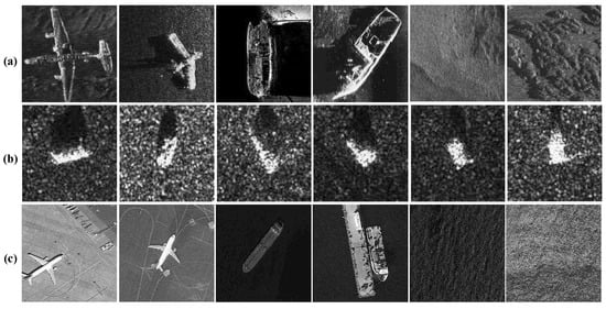
Figure 7.
The datasets used in the experiments: (a) SSS image samples; (b)SAR image samples; (c) Grayscale optical image samples.
The transfer learning approach proposed in this paper exploits two other related datasets. The SAR dataset is selected from the MSATR dataset. MSTAR was introduced in the mid-1990s by the US Defense Advanced Research Projects Agency (DARPA). The SAR imagery of a wide range of former Soviet target military vehicles was acquired via high-resolution, cluster-beam synthetic aperture radar. The categories of targets in SAR images are not related to SSS images. However, the similarity of image statistical features between the two datasets deserves our attention. Therefore, we tried to train the feature extraction module of VGG19 on the SAR dataset and transfer it to the SSS image classification network to improve the extraction of low-level detailed features from strong noise. The optical dataset is made up of optical aerial images, including ships and sea surface images in MAritime SATellite Imagery dataset (MASATI), and airplane images in Dataset of Object Detection in Aerial Images (UCAS-AOD). This conventional optical dataset is used to train the feature mapping module in the optical image classification network, which will be transferred to the SSS image classification network. The feature mapping module contains the FC layers close to outputs, in which the majority of parameters are concentrated.
3.1.2. Experimental Details
For each class of the SeabedObjects-KLSG-II dataset, 70% and 30% of the images were randomly selected as training and test samples respectively. The numbers of training samples and testing samples are shown in the Table 1. To eliminate possible influence of sample partitioning on the performance of the classifier, a hold-out scheme was used to randomly create 10 datasets to test the classifier. To minimize the impact of random initialization of parameters, 10 test repetitions are conducted on each dataset and the average value is taken as the result of the classification on this dataset. The average value of the results on the 10 datasets is taken as the final result.

Table 1.
Division situation of SeabedObjects-KLSG-II dataset.
Due to the small size of the SSS image dataset, several basic data enhancement methods—including flipping, rotating, cropping, and stitching—were used, which are shown in Figure 8. In practice, the target in the image acquired by the side-scan sonar may be at the edge of the image, or even mutilated. The enhanced dataset obtained by using cropping and stitching more closely resembles the actual sonar images, giving the model a stronger generalization capability.
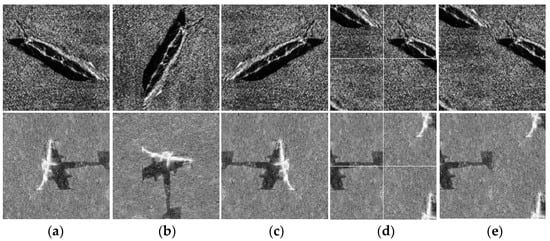
Figure 8.
Sample examples of basic data enhancement methods: (a) original image sample; (b) flipping sample; (c) rotating sample; (d) cropping samples; (e) cropping and stitching sample.
Before parameter transfer, we need to train the source domain models with SAR image and grayscale optical image datasets. Pretrained VGG19 on ImageNet was used to save time significantly. Some training hyper-parameters were set as: the batch size was 16, the epochs were 15, and the initial learning rate was 0.001 which will be multiplied by a decay factor 0.1 after 10 epochs. Constraint coefficients of source domain models were set according to the Formula (4).
In the training process, the training samples were first input into the detector to generate the feature map by feature extraction modules of Backbone. Then, the feature maps were enhanced and fused by RAM for a better representation, and were mapped from feature space to label space by FC layers. Afterwards, the loss value was calculated between the predicted label vector and the true label to evaluate the performance of the model’s parameters in predicting target category information. Finally, the parameters of the model were updated using the stochastic gradient descent (SGD) algorithm.
Some training hyper-parameters were set as: the initial learning rate was 0.0001, the batch size was 16, the epochs were 20, and the probability of dropout scheme was 0.5. The weighted learning rate and the bias learning rate were both set to 20 to accelerate the learning of parameters for the newly added final fully connected layer. For the method of using bag of features (BOF) model on SIFT features with SVM as the classifier, the size of BOF was set to 300.
3.2. Network Model Evaluating Indicator
The criteria for assessing model performance are the average overall accuracy (OA), the variance OA, and the precision of each class.
The overall accuracy (OA), which is the percentage of all correct positive classifications, represents the overall classification performance; the variance of the overall accuracy demonstrates the stability of the model over multiple tasks; and the analysis of the accuracy of each class is necessary because of the intra-class imbalance in the dataset. In addition, as we also judge from the convergence curve of the model whether or not over-fitting occurs.
where Nii is the number of test samples that should have been classified as class i and were classified as class i in the actual classification result, and t means the categories of labels in test samples.
Using the airplane target as an example, TP (true positive) indicates that the model predicts that there is an airplane, and the result is true; FP (false positive) indicates that the content of the predicted target is an airplane, but it is not true. In short, precision means the proportion of correctly predicted results in all the samples whose predicted label is true.
Variance is used to measure the stability and robustness of the algorithm, which can be obtained by comparing the results of multiple experiments with their mean values.
3.3. Performance Analysis
The model is constructed using the training set and verification set divided by 10 times cross validation strategy. The final performance is measured according to each performance index in the test dataset.
As shown in Table 2, we compared state-of-the-art (SOTA) methods [3,8,9,27,28,29] with our method and listed their details and performance. The CNN models based on LeNet-5 [9] and GoogLeNet [27] are super lightweight and easy to train, while their performance is unsatisfactory for practical use. Various data enhancement methods are used in these SOAT methods including semisynthetic data generation [3,8], despeckling [28], and extracting derived classification dataset [29], which greatly improve the classification accuracy but cause more time consumption. For example, the effective FL-DARTS [29] algorithm, which also uses radar and sonar datasets together, have close classification performance to our method, but excessive complexity and training time of auto learning presents obstacles to its wider use in underwater tasks. Compared with these existing methods, our proposed transfer learning method has significant performance improvement and competitive classification speed with acceptable complexity and training time.
Table 2.
Comparison of methods for the classification of SSS images.
Table 3 shows quantitative results comparing different backbone networks on the SeabedObjects-KLSG test set for the target classification task. By comparison, we found that the VGG19 network exhibited good generalization performance after fine-tuning. Fine-tuned VGG19 achieved the highest overall accuracy and the highest precision of the classification of ship and seafloor. Although VGG16 has a significantly better precision of airplane classification, it got the worst precision of seafloor classification, which means it has a high false alarm rate. Compared with VGG16, VGG19 has three more convolutional layers, which makes it more suitable to be combined with the proposed MSRAM that can work better with a deeper model structure. By using a deeper network structure likeVGG19, the proposed MSRAM can combine more multi-scale features to improve the feature representation ability.
Table 3.
Comparison of different fine-tuning backbones for the classification of SSS image.
Ablation experiments on different methods of transfer learning were conducted to verify the performance improvement as well as the stability of transfer learning for the SSS image classification task, 10 times for each method, and calculated the average and the variance of the overall accuracy. As can be seen from the results in the Table 4 below, the model achieved a good improvement after transferring parameters from the SAR dataset alone, indicating that the similarity of the low-level features between SAR images and SSS images makes the model learn the extracted features in advance. To confirm this, we used a feature response visualization approach to observe the performance improvement owing to transfer learning from the SAR dataset. Transfer learning from optical datasets likewise improved the model overall accuracy, while resulting in significant instability which can be seen from the highest variance. Although transfer learning from both SAR and optical data sets enables further performance improvements, the model was still instable compared to the baseline model. MSRAM is therefore introduced to stabilize the learned feature extraction and mapping capabilities from multi-domain transfer learning. The method of MCDTL with MSRAM finally got the best classification accuracy and the lowest variance, which means it was able to eliminate performance fluctuations and maintain optimum performance.
Table 4.
Comparison of different transfer learning methods.
However, we found that the model had poor ability to recognize and classify airplanes, which resulted from the class imbalance in the SSS image dataset. To investigate the effect of the proposed method on different target classes, we observed the precision corresponding to the classes.
As can be seen from the boxplots in Figure 9 below, when training directly from scratch using VGG19, the classification of the airplane category is poor and unstable, with the best result not even reaching 65%, although the OA reaches over 90%. The direct fine-tuning and transfer learning methods were used to improve the classification accuracy, but it can be seen that results are worse in the degree of fluctuation, which indicates that the model performance is not stable enough. This may be due to the fact that there are fewer airplane images and the scarce training set cannot meet the learning needs of the model, while the model does not fully learn the detailed information of the target, and when there is a change in the posture of the airplane, the model is unable to capture the key information. The proposed method of combining MDCTL with RAM not only improves the accuracy rate in all categories as well as in general, but also makes the classification model more stable.
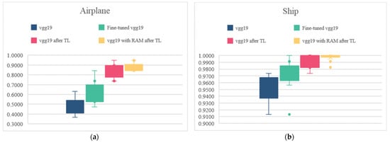
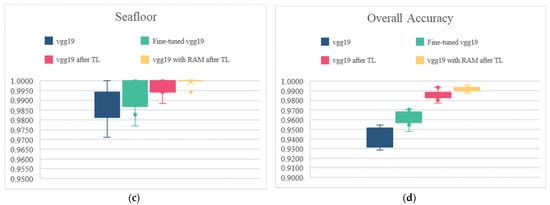
Figure 9.
Box plots of the precision of each category and overall accuracy using different methods: (a) Classification precision of airplane; (b) Classification precision of ship; (c) Classification precision of seafloor; (d) Overall accuracy.
3.4. Visualization
3.4.1. Feature Response Map Visualization
Given that edge features and detailed information of the target can be better extracted from the convolutional layers close to the input, we visualized the first convolutional layer response of four models, including unpre-trained VGG19, pre-trained VGG19 based on the ImageNet, VGG19 learned from the SAR classification model, and a model with RAM added after TL. The details of the visualization method are shown in Figure 10.
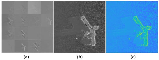
Figure 10.
Feature response maps and that after staining: (a) Feature maps of the first 16 channels of the first convolution layer; (b) The superimposition map of feature maps of all channel responses; (c) The stain chart of (b).
The Figure 11b–d can show how the four methods gradually distinguish the highlighted and shadowed areas of the image from the background noise, where Figure 11d further improves the ability to extract detailed features from the wreck target compared to Figure 11c. As shown in Figure 11e, the detailed contours in the target highlight area and the shadow contours become clearer with the addition of MSRAM, and seafloor highlight area is suppressed. MSRAM makes the edge contour details of the target and the edge features of the shadows significantly extracted, while the highlight areas of the seabed unrelated to the wreck are suppressed.
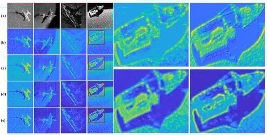
Figure 11.
Comparison of feature response maps for different models: (a) SSS image samples; (b) Pre-trained VGG19 using ImageNet; (c) Retrain the pre-trained VGG19; (d) VGG19 transfer learned from SAR dataset; (e) VGG19 with MSRAM after transfer learning. The four images on the right are partial enlargements within the red box.
3.4.2. Heat Maps Based on Grad-CAM
The VGG19 network can be considered as a feature extraction module combined with a feature mapping module. As the feature extraction module can be transferred, we also tried to apply transfer learning on the feature mapping module, that is, the fully connected layers block. In the VGG19 network model, the fully connected layers play the role of mapping the learned distributed feature representation to the sample label space. The fully connected layers become very sensitive to the structural information of the image, such as the outline, so we transferred this part trained on the optical image dataset which have the same category and target semantic information. We use Grad-CAM (Gradient Weighted Class Activation Mapping) to visualize the areas of focus of the fully connected layer on the different classes, i.e., the influence of the structural information of the image on the classification results.
From the class activation heatmaps in Figure 12, it can be seen that the aerial images and sonar images of the same category have similar contour features, and the feature details that the model pays attention to are similar in classification. For example, in the group of the airplane category, the features that have a positive impact on the category classification are concentrated on the edges of the wings on both sides of the airplane and the connection between the wings and the fuselage. This demonstrates that when training the classification decision module, although the image modalities are different, the images of the same object category have the same contour information, which can provide a certain gain effect for training.
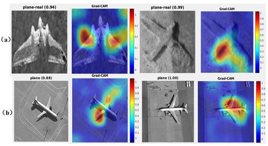
Figure 12.
Class activation heatmaps of airplane classification in SSS images and optical images: (a) Heatmaps of SSS images; (b) Heatmaps of optical images.
The similarity of the airplane class activation heat maps between the SSS image and optical image shows that the feature mapping module focuses on consistent features of the airplane. Traditional classification networks can achieve target recognition and classification by focusing only on the corresponding key features of the category, such as the wings or the tail of the airplane. However, for small SSS image datasets, the model cannot learn all the key features of each category with sufficient samples, and therefore adequate learning of each sample is necessary. The MDCTL proposed in this paper makes use of the feature mapping module of the optical image classification model to learn as much as key information as possible that is required to complete recognition and classification which contribute to classifying the same category. Moreover, the MSRAM is used to pass the high-level spatial contour information to the front-end channel attention mechanism at different levels, enabling the acquisition of rich features at key locations at the feature extraction stage. To verify the effectiveness of the proposed method, we observed the class activation heat maps on different methods, which are given in Figure 13. Figure 13 illustrates that the classification results and the accuracy of the selected airplane samples are greatly improved after using the MDCTL method, and information on key locations is also focused on. As shown in Figure 13d, after adding MSRAM, the model pays more attention to the comprehensive and holistic feature information of the target, which is exactly what we need.
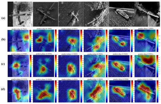
Figure 13.
Class activation heatmaps using different methods: (a) SSS image samples (b) Heatmaps using directly fine-tuning; (c) Heatmaps using MDCTL; (d) Heatmaps using MDCTL with MSRAM.
3.5. Details in MCDTL
However, due to the small size of the SSS image dataset in the target domain, the selection of the size of the multi-domain dataset is very critical. If the size of the source domain dataset is too large, overfitting will occur, which will make it more difficult to migrate the model to the task of sonar image target classification; if the dataset is too small, the migrated model will not achieve the desired results. To address this issue, we selected SAR and optical datasets of five different sizes relative to the SSS dataset 0.5×, 1×, 1.5×, 3×, and 5× for transfer learning, and the experimental results are shown in Figure 14.
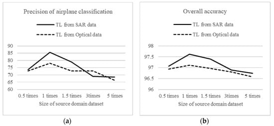
Figure 14.
Experimental results of the different sizes of source domain datasets on migration learning: (a) Precision of airplane classification; (b) Overall accuracy.
From Figure 14, it can be seen that the model performance curve reaches the peak when the two datasets are about the same size, and that the curve begins to degrade when the size of the source domain dataset exceeds that of the target domain dataset. The reason for this is that when the size of the source domain dataset becomes larger than that of the target domain dataset, the parameters of the trained model tend to be closer to those used in the source domain classification task. Therefore, to obtain the optimal result, only a part of the source domain dataset with the same size as that of the target domain dataset is selected.
Table 5 shows the differences between the different transfer learning methods and the number of convolutional layers for parametric transfer learning with the SAR dataset. We can obtain the highest accuracy by transferring the first two convolutional blocks and retraining the parameters. The first two convolutional blocks can be considered as a feature extractor which can extract more accurate and rich edge features from noisy and complex images after pre-training on the SAR dataset. It is necessary for the transferred module to be retrained to be adapted to the target task.
Table 5.
Comparison of different transfer learning methods using SAR datasets.
3.6. Applications for Detection
The proposed method aims to speed up the search for underwater targets with automated classification algorithms, and it can also be combined with region proposal network (RPN) to detect objects in SSS images. To verify the effectiveness of the proposed method, we applied it to mine detection and compared its detection performance with several recent SOTA algorithms [1,2] used for underwater target detection, and the comparative results are shown in Table 6.
Table 6.
Comparison with SOTA algorithms in mine detection.
Our method was combined with RPN which is used in the detection head for generating proposal regions. The multi-scale structure of MSRAM can match RPN well. Therefore, the detection method of transfer learning with MSRAM can accurately locate the target position, which can be seen in Figure 15. Transfer learning from the SAR dataset with MSRAM outperformed other SOTA methods in terms of AP@0.5 and average IOU, while its computational complexity and detecting speed need to be improved. Currently, only a small size of the mine class dataset—which includes 152 mine objects in total—is available, and in the future we will try to do more experiments and collect more samples to verify and improve our method.
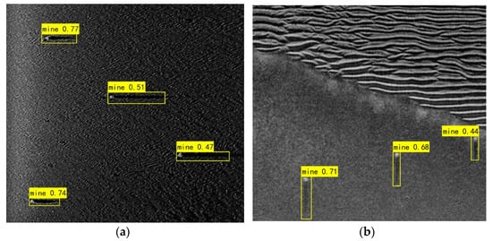
Figure 15.
Experimental results of mine detection using SARTL combined with MSARM: (a) Mines on rippled seabed; (b) Mines near sand ridges.
4. Discussion
4.1. Significance of the Proposed Method
The MDCTL-MSRAM proposed in this paper provides an improvement for underwater target classification in SSS images, which is important for underwater applications—such as emergency search, sea rescue, wreck recovery, and military defense—or other unmanned devices that require target object detection and classification.
Multi-domain collaborative transfer learning (MDCTL) is introduced to alleviate the problem of scarcity of training datasets. It utilizes the SAR image datasets and the optical image datasets to improve the learning effect of different modules, which will increase the classification accuracy of the model. It also brings new inspiration about how to perform transfer learning effectively from multi-domain datasets of different categories but correlative features to target domain.
The multi-scale repeated attention mechanism (MSRAM) is introduced to make the model more focused on the target or regions near the target and increase the proportion of channels with higher feature extraction ability to obtain richer edge texture and contour detail features with the exclusion of noise. MSRAM is able to capture the abundant range of features in or around the target, ensuring that the network achieves better generalization in limited training samples.
4.2. Limitations of the Proposed Method
Although the proposed MDCTL-MSRAM method achieves better performance than direct fine-tuning in the above experiments, it is more complex than fine-tuning. The pre-training of two different modal datasets in the first stage, together with the retraining process of the sonar datasets, takes nearly twice as long as direct fine-tuning the model.
In addition, category imbalance of SSS dataset has not been considered in the proposed method. The least numerous class compared to the others is the airplane class, which is the typical ‘long-tail class’, and it will cause a negative impact on the stability of the model convergence when there are poor-quality samples in the class. There are several misclassified SSS images which even cannot be judged accurately by humans, as shown in Figure 16a,b.
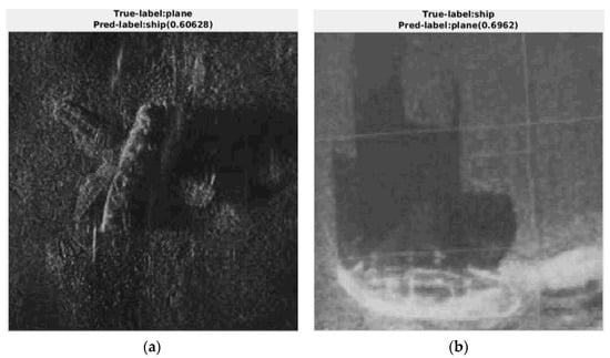
Figure 16.
Misclassification samples: (a) A sample of an airplane which was misclassified as a ship; (b) A sample of a ship which was misclassified as an airplane.
5. Conclusions
A multi-domain collaborative transfer learning method with a multi-scale repeated attention mechanism is proposed in this paper for underwater sonar image classification. Considering the feature similarity of the multi-domain datasets, concretely the similarity of noise features between sonar and SAR images and the similarity of class shape features between sonar and optical images, the SAR datasets and the optical datasets are used for transfer learning, which ultimately improve the capabilities of feature extraction and mapping of the SSS images. A repeated attention mechanism, which combines the space and the channel attention modules, is used to further extract rich contour information from the target extensively for the problem that small batches of training samples are not sufficient for training to achieve optimal classification accuracy and generalization capability of the model. Experimental results and visualized maps show that our method can extract more features at key target locations effectively, which have a 4.54% improvement of overall accuracy compared with the direct fine-tuning. The proposed method improves the efficiency and accuracy of SSS image classification and offers a new way for transfer learning using multi-domain datasets based on the similarity of data features.
Author Contributions
Conceptualization, Z.C. and G.H.; Methodology, Z.C. and G.H.; Software, Z.C.; Validation, Z.C. and G.H.; Formal analysis, Z.C. and G.H.; Investigation, Z.C. and G.H.; Resources, G.H.; Data curation, G.H.; Writing—original draft preparation, Z.C.; Writing—review and editing, Z.C. and G.H.; Visualization, Z.C.; Supervision, G.H. and H.L.; Project administration, G.H. and H.L.; Funding acquisition, G.H. All authors have read and agreed to the published version of the manuscript.
Funding
This research was funded by National Natural Science Foundation of China under grant nos. 41876097 and U1906218; in part by the Scientific Research Fund of the Second Institute of Oceanography, Ministry of Natural Resources (MNR), under grant no. JB1803.; and in part by Key R & D plan of Jiangsu Province under grant no. BE2019036.
Institutional Review Board Statement
Not applicable.
Informed Consent Statement
Not applicable.
Data Availability Statement
Access to the data will be available at https://github.com/HHUCzCz/-SeabedObjects-KLSG--II (accessed on 16 November 2021).
Acknowledgments
We would like to thank L-3 Klein Associates, EdgeTech, Lcocean, Hydro-tech Marine, and Tritech for their great support for providing the valuable real side-scan sonar images.
Conflicts of Interest
The authors declare no conflict of interest.
References
- Kong, W.Z.; Hong, J.C.; Jia, M.Y.; Yao, J.L.; Gong, W.H.; Hu, H.; Zhang, H.G. YOLOv3-DPFIN: A Dual-Path Feature Fusion Neural Network for Robust Real-Time Sonar Target Detection. IEEE Sens. J. 2020, 20, 3745–3756. [Google Scholar] [CrossRef]
- Yu, Y.C.; Zhao, J.H.; Gong, Q.H.; Huang, C.; Zheng, G.; Ma, J.Y. Real-Time Underwater Maritime Object Detection in Side-Scan Sonar Images Based on Transformer-YOLOv5. Remote Sens. 2021, 13, 3555. [Google Scholar] [CrossRef]
- Ye, X.; Li, C.; Zhang, S.; Yang, P.; Li, X. Research on side-scan sonar image target classification method based on transfer learning. In Proceedings of the OCEANS 2018 MTS/IEEE, Charleston, SC, USA, 22–25 October 2018; pp. 1–6. [Google Scholar]
- Vandrish, P.; Vardy, A.; Walker, D.; Dobre, O. Side-scan sonar image registration for AUV navigation. In Proceedings of the 2011 IEEE Symposium on Underwater Technology and Workshop on Scientific Use of Submarine Cables and Related Technologies, Tokyo, Japan, 5–8 April 2011; pp. 1–7. [Google Scholar]
- Zerr, B.; Stage, B.; Guerrero, A. Automatic Target Classification Using Multiple Sidescan Sonar Images of Different Orientations; NATO, SACLANT Undersea Research Centre: La Spezia, Italy, 1997. [Google Scholar]
- Chew, A.L.; Tong, P.B.; Chia, C.S. Automatic detection and classification of man-made targets in side scan sonar images. In Proceedings of the 2007 Symposium on Underwater Technology and Workshop on Scientific Use of Submarine Cables and Related Technologies, Tokyo, Japan, 17–20 April 2007; pp. 126–132. [Google Scholar]
- Tellez, O.L. Underwater threat recognition: Are automatic target classification algorithms going to replace expert human operators in the near future? In Proceedings of the OCEANS 2019, Marseille, France, 17–20 June 2019; pp. 1–4. [Google Scholar]
- Huo, G.Y.; Wu, Z.Y.; Li, J.B. Underwater Object Classification in Sidescan Sonar Images Using Deep Transfer Learning and Semisynthetic Training Data. IEEE Access 2020, 8, 47407–47418. [Google Scholar] [CrossRef]
- Luo, X.W.; Qin, X.M.; Wu, Z.Y.; Yang, F.L.; Wang, M.W.; Shang, J.H. Sediment Classification of Small-Size Seabed Acoustic Images Using Convolutional Neural Networks. IEEE Access 2019, 7, 98331–98339. [Google Scholar] [CrossRef]
- Chaillan, F.; Fraschini, C.; Courmontagne, P. Speckle noise reduction in SAS imagery. Signal Process. 2007, 87, 762–781. [Google Scholar] [CrossRef]
- Kazimierski, W.; Zaniewicz, G. Determination of Process Noise for Underwater Target Tracking with Forward Looking Sonar. Remote Sens. 2021, 13, 1014. [Google Scholar] [CrossRef]
- Buslaev, A.; Iglovikov, V.I.; Khvedchenya, E.; Parinov, A.; Druzhinin, M.; Kalinin, A.A. Albumentations: Fast and flexible image augmentations. Information 2020, 11, 125. [Google Scholar] [CrossRef]
- Ghannadi, M.A.; Saadaseresht, M. A modified local binary pattern descriptor for SAR image matching. IEEE Geosci. Remote Sens. Lett. 2018, 16, 568–572. [Google Scholar] [CrossRef]
- Wilson, P.I.; Fernandez, J. Facial feature detection using Haar classifiers. J. Comput. Sci. Coll. 2006, 21, 127–133. [Google Scholar]
- Yang, F.; Xu, Q.Z.; Li, B. Ship Detection from Optical Satellite Images Based on Saliency Segmentation and Structure-LBP Feature. IEEE Geosci. Remote Sens. Lett. 2017, 14, 602–606. [Google Scholar] [CrossRef]
- Huang, H.; Guo, W.; Zhang, Y. Detection of copy-move forgery in digital images using SIFT algorithm. In Proceedings of the 2008 IEEE Pacific-Asia Workshop on Computational Intelligence and Industrial Application, Wuhan, China, 19–20 December 2008; pp. 272–276. [Google Scholar]
- Sun, Y.; Zhao, L.; Huang, S.; Yan, L.; Dissanayake, G. L2-SIFT: SIFT feature extraction and matching for large images in large-scale aerial photogrammetry. ISPRS J. Photogramm. Remote Sens. 2014, 91, 1–16. [Google Scholar] [CrossRef]
- Lakshmi, M.D.; Raj, M.V.; Murugan, S.S. Feature matching and assessment of similarity rate on geometrically distorted side scan sonar images. In Proceedings of the 2019 TEQIP III Sponsored International Conference on Microwave Integrated Circuits, Photonics and Wireless Networks (IMICPW), Tiruchirappalli, India, 22–24 May 2019; pp. 208–212. [Google Scholar]
- Myers, V.; Fawcett, J. A Template Matching Procedure for Automatic Target Recognition in Synthetic Aperture Sonar Imagery. IEEE Signal Process. Lett. 2010, 17, 683–686. [Google Scholar] [CrossRef]
- Reed, S.; Petillot, Y.; Bell, J. An automatic approach to the detection and extraction of mine features in sidescan sonar. IEEE J. Ocean. Eng. 2003, 28, 90–105. [Google Scholar] [CrossRef]
- Seymore, K.; McCallum, A.; Rosenfeld, R. Learning hidden Markov model structure for information extraction. In Proceedings of the AAAI-99 Workshop on Machine Learning for Information Extraction, Orlando, FL, USA, 18–19 July 1999; pp. 37–42. [Google Scholar]
- Dobeck, G.J.; Hyland, J.C. Automated detection and classification of sea mines in sonar imagery. In Proceedings of the Detection and Remediation Technologies for Mines and Minelike Targets II, Orlando, FL, USA, 22 July 1997; pp. 90–110. [Google Scholar]
- Wan, S.A.; Yeh, M.L.; Ma, H.L. An Innovative Intelligent System with Integrated CNN and SVM: Considering Various Crops through Hyperspectral Image Data. ISPRS Int. J. Geo-Inf. 2021, 10, 242. [Google Scholar] [CrossRef]
- Çelebi, A.T.; Güllü, M.K.; Ertürk, S. Mine detection in side scan sonar images using Markov Random Fields with brightness compensation. In Proceedings of the 2011 IEEE 19th Signal Processing and Communications Applications Conference (SIU), Antalya, Turkey, 20–22 April 2011; pp. 916–919. [Google Scholar]
- Girshick, R.; Donahue, J.; Darrell, T.; Malik, J. Rich feature hierarchies for accurate object detection and semantic segmentation. In Proceedings of the IEEE Conference on Computer Vision and Pattern Recognition, Columbus, OH, USA, 23–28 June 2014; pp. 580–587. [Google Scholar]
- Ren, S.; He, K.; Girshick, R.; Sun, J. Faster R-CNN: Towards Real-Time Object Detection with Region Proposal Networks. IEEE Trans. Pattern Anal. 2017, 39, 1137–1149. [Google Scholar] [CrossRef] [PubMed]
- Qin, X.M.; Luo, X.W.; Wu, Z.Y.; Shang, J.H. Optimizing the Sediment Classification of Small Side-Scan Sonar Images Based on Deep Learning. IEEE Access 2021, 9, 29416–29428. [Google Scholar] [CrossRef]
- Gerg, I.D.; Monga, V. Structural Prior Driven Regularized Deep Learning for Sonar Image Classification. IEEE Trans. Geosci. Remote Sens. 2021, 60, 1–16. [Google Scholar] [CrossRef]
- Zhang, P.; Tang, J.S.; Zhong, H.P.; Ning, M.Q.; Liu, D.D.; Wu, K. Self-Trained Target Detection of Radar and Sonar Images Using Automatic Deep Learning; IEEE: Piscataway, NJ, USA, 2021. [Google Scholar]
- Inoue, H. Data augmentation by pairing samples for images classification. arXiv 2018, arXiv:1801.02929. [Google Scholar]
- Barngrover, C.; Kastner, R.; Belongie, S. Semisynthetic versus real-world sonar training data for the classification of mine-like objects. IEEE J. Ocean. Eng. 2014, 40, 48–56. [Google Scholar] [CrossRef][Green Version]
- Ge, Q.; Ruan, F.X.; Qiao, B.J.; Zhang, Q.; Zuo, X.Y.; Dang, L.X. Side-Scan Sonar Image Classification Based on Style Transfer and Pre-Trained Convolutional Neural Networks. Electronics 2021, 10, 1823. [Google Scholar] [CrossRef]
- Li, C.L.; Ye, X.F.; Cao, D.X.; Hou, J.; Yang, H.B. Zero shot objects classification method of side scan sonar image based on synthesis of pseudo samples. Appl. Acoust. 2021, 173, 107691. [Google Scholar] [CrossRef]
- Steiniger, Y.; Kraus, D.; Meisen, T. Generating Synthetic Sidescan Sonar Snippets Using Transfer-Learning in Generative Adversarial Networks. J. Mar. Sci. Eng. 2021, 9, 239. [Google Scholar] [CrossRef]
- Sung, M.; Cho, H.; Kim, J.; Yu, S.-C. Sonar image translation using generative adversarial network for underwater object recognition. In Proceedings of the 2019 IEEE Underwater Technology (UT), Kaohsiung, Taiwan, 16–19 April 2019; pp. 1–6. [Google Scholar]
- Pan, S.J.; Yang, Q. A survey on transfer learning. IEEE Trans. Knowl. Data Eng. 2009, 22, 1345–1359. [Google Scholar] [CrossRef]
- Hasan, M.S. An application of pre-trained CNN for image classification. In Proceedings of the 2017 20th International Conference of Computer and Information Technology (ICCIT), Dhaka, Bangladesh, 22–24 December 2017; pp. 1–6. [Google Scholar]
- Schwarz, M.; Schulz, H.; Behnke, S. RGB-D object recognition and pose estimation based on pre-trained convolutional neural network features. In Proceedings of the 2015 IEEE International Conference on Robotics and Automation (ICRA), Seattle, WA, USA, 25–30 May 2015; pp. 1329–1335. [Google Scholar]
- Lasloum, T.; Alhichri, H.; Bazi, Y.; Alajlan, N. SSDAN: Multi-Source Semi-Supervised Domain Adaptation Network for Remote Sensing Scene Classification. Remote Sens. 2021, 13, 3861. [Google Scholar] [CrossRef]
- Rostami, M.; Kolouri, S.; Eaton, E.; Kim, K. Sar image classification using few-shot cross-domain transfer learning. In Proceedings of the IEEE/CVF Conference on Computer Vision and Pattern Recognition Workshops, Long Beach, CA, USA, 16–20 June 2019. [Google Scholar]
- Li, X.Y.; Zhang, L.F.; You, J.N. Domain Transfer Learning for Hyperspectral Image Super-Resolution. Remote Sens. 2019, 11, 694. [Google Scholar] [CrossRef]
- Rusu, A.A.; Rabinowitz, N.C.; Desjardins, G.; Soyer, H.; Kirkpatrick, J.; Kavukcuoglu, K.; Pascanu, R.; Hadsell, R. Progressive neural networks. arXiv 2016, arXiv:1606.04671. [Google Scholar]
- Woo, S.; Park, J.; Lee, J.-Y.; Kweon, I.S. Cbam: Convolutional block attention module. In Proceedings of the European Conference on Computer Vision (ECCV), Munich, Germany, 8–14 September 2018; pp. 3–19. [Google Scholar]
- Park, J.; Woo, S.; Lee, J.-Y.; Kweon, I.S. Bam: Bottleneck attention module. arXiv 2018, arXiv:1807.06514. [Google Scholar]
- Niu, X.X.; Suen, C.Y. A novel hybrid CNN-SVM classifier for recognizing handwritten digits. Pattern Recognit. 2012, 45, 1318–1325. [Google Scholar] [CrossRef]
- Itti, L.; Koch, C.; Niebur, E. A model of saliency-based visual attention for rapid scene analysis. IEEE Trans. Pattern Anal. 1998, 20, 1254–1259. [Google Scholar] [CrossRef]
- Hu, J.; Shen, L.; Sun, G. Squeeze-and-excitation networks. In Proceedings of the IEEE Conference on Computer Vision and Pattern Recognition, Salt Lake City, UT, USA, 18–23 June 2018; pp. 7132–7141. [Google Scholar]


Publisher’s Note: MDPI stays neutral with regard to jurisdictional claims in published maps and institutional affiliations. |
© 2022 by the authors. Licensee MDPI, Basel, Switzerland. This article is an open access article distributed under the terms and conditions of the Creative Commons Attribution (CC BY) license (https://creativecommons.org/licenses/by/4.0/).