Abstract
The recent development and miniaturization of hyperspectral sensors embedded in drones has allowed the acquisition of hyperspectral images with high spectral and spatial resolution. The characteristics of both the embedded sensors and drones (viewing angle, flying altitude, resolution) create opportunities to consider the use of hyperspectral imagery to map and monitor macroalgae communities. In general, the overflight of the areas to be mapped is conconmittently associated accompanied with measurements carried out in the field to acquire the spectra of previously identified objects. An alternative to these simultaneous acquisitions is to use a hyperspectral library made up of pure spectra of the different species in place, that would spare field acquisition of spectra during each flight. However, the use of such a technique requires developed appropriate procedure for testing the level of species classification that can be achieved, as well as the reproducibility of the classification over time. This study presents a novel classification approach based on the use of reflectance spectra of macroalgae acquired in controlled conditions. This overall approach developed is based on both the use of the spectral angle mapper (SAM) algorithm applied on first derivative hyperspectral data. The efficiency of this approach has been tested on a hyperspectral library composed of 16 macroalgae species, and its temporal reproducibility has been tested on a monthly survey of the spectral response of different macro-algae species. In addition, the classification results obtained with this new approach were also compared to the results obtained through the use of the most recent and robust procedure published. The classification obtained shows that the developed approach allows to perfectly discriminate the different phyla, whatever the period. At the species level, the classification approach is less effective when the individuals studied belong to phylogenetically close species (i.e., Fucus spiralis and Fucus serratus).
1. Introduction
Macroalgae communities represent an essential component of the coastal environment as they play a major role as mating and nursery grounds [1,2], feeding areas [3], and refuges [4] for many species. Furthermore, their contribution to the coastal primary productivity is no longer to be demonstrated [5,6] with an assimilation of carbon an order of magnitude higher than the one of phytoplankton [7]. In coastal areas, macroalgae are mainly present on rocky shores, and, as sessile organisms, they have to cope with the alternation between aerial and aquatic environments. The transition between the marine and aerial environment generates a stress gradient, increasing from the low shore to the high shore, related to different environmental parameters, including irradiance, dessication, and temperature [8,9]. One consequence of this vertical gradient is the distribution of species along the shore, according to their ability to cope with environmental stress. In macroalgae, variations in both light intensity and quality along this gradient are mainly expressed by the occurrence of three different phyla of algae, which are partly characterized by different pigment contents. The first one is the phylum of Chlorophyta (green algae), characterized by a pigment content similar to higher plants. These algae are generally located in the upper shore, where emersion periods are long-lasting. On the contrary, the second group, composed of Rhodophyta (red algae), is located on the lower shore where the emersion periods are short-lasting and occasional. Red algae get their name from red-colored accessory pigments, i.e., the phycobiliproteins. The third phylum is the Ochrophyta (brown algae) which contains the largest sized species, found all along the shore. Brown algae species are vertically distributed according to the tidal levels, forming belts of typical species. This zonation pattern is observed worldwide in temperate areas [10]. Moreover, in terms of primary productivity, brown algae are among the most productive biological system per unit area [11] and “kelp forests” (i.e., brown algae belonging to Laminariales) have even been considered equivalent to the terrestrial rain forests [12]. Macroalgae are particularly sensitive to the impact of human activities and the resulting climate change [13]. In particular, a decline in brown seaweed communities has been observed in recent decades [14,15,16,17,18], and may be accompanied by a change in community composition. In particular, the so-called canopy-forming species are more sensitive to climate change [19] and, when declining, can give way to “turf algae” species, composed of green or red algae [20,21]. These species have been shown to be generally less productive and do not provide the ecosystem services provided by canopy communities, such as nursery or breeding ground [22]. However, more information is needed to better understand the different phenomena responsible for this decline as well as the long-term evolution of the communities [23,24].
In order to understand and monitor the effect of anthropogenic activities and global change on the distribution and composition of macroalgal communities, accurate mapping of the different species distribution is still needed. Until recently, when possible, mapping had been performed with traditional techniques that involved field surveys based on estimates of species abundances within quadrats. However, this approach is considered expensive [25,26,27], time-consuming, and not applicable for traditional field sampling for mapping macroalgae at large spatial scales [28]. To overcome this problem, aerial photography techniques were developed in the early 1980s, which quickly showed their limitations, mainly due to difficulties in interpreting the results and the associated cost [29,30]. In the 1990s, easy access to satellite images from multispectral sensors allowed the development of qualitative and quantitative mapping techniques. However, these techniques are limited by the number of acquirable broad bands (commonly three to ten spectral bands) that do not allow accurate species discrimination. The advent of hyperspectral remote sensing technology has allowed a better acquisition of the spectral properties of observed surfaces, by the acquisition of a large number of contiguous and narrow spectral bands, which provided a more accurate identification of the observed objects. Bajjouk et al. [25] were among the first to demonstrate the usefulness of spectral imaging for discrimination of the three macroalgal phyla through the use of spectral bands in the visible wavelength range. Since, several studies have shown the separability capacity of spectral imagery to perform macroalgae discrimination in different environmental conditions. However, these studies have generally focused on the discrimination of macroalgae from other types of plants or substrates, such as algae associated with coral reefs [31,32,33], monitoring seaweed invasions [34] or mapping large monospecific areas [26,35,36,37,38]. Following the development of hyperspectral imaging, the improvement of unmanned aerial vehicles (UAVs), and in particular copter drones, has rapidly attracted the interest of the scientific community, due to their ease of deployment and low cost [39,40]. In addition, the miniaturization of sensors made it possible to equipped UAVs with hyperspectral cameras to capture hyperspectral images [41,42], and in particular thanks to their low flight height (30 m), drones allow the acquisition of high spatial resolution images.
To perform macroalgae species discrimination, it is necessary to obtain spectral information for macroalgal species. Usually, mapping is associated with in situ reflectance spectrum collection directly performed on various natural surfaces for acquiring a set of references for each studied species. However, this data collection is not always feasible due to difficulty to access (e.g., large size rocks), and requires additional efforts during the mapping campaign. The constitution of a spectral library based on the species occurring in the study area seems to be an interesting alternative to field measurements [43]. Despite the advantages of such a technique, there are still only a few publications referring to macroalgal spectral libraries [27,44,45,46,47,48]. Preliminary works have already been undertaken to evaluate the possibility of discriminating individuals belonging to different species. For example, Chao Rodríguez et al. [47] compared the effectiveness of three techniques (RGB-colorimetry, true skill statistics optimal band (TSS-OB), and derivative spectroscopy) for classifying hyperspectral signatures of different species but they only succeeded in discriminating the individuals at the phylum level (green, brown, and red), but not at the species level. More recently, Olmedo-Masat et al. [27] showed that species discrimination was possible using analysis of a macroalgae spectral library of 28 macroalgae from the southwest Atlantic. However, in the majority of studies based on a spectral library feature [43], intra-species variability is not taken into account due to pre-processing applied to the data sets (mean, median, etc.). Furthermore, the seasonal variation is another important parameter that is generally not taken into account in most of these studies. Indeed, it has been shown that the reflectance properties of vegetation vary over time [49]. However, very few studies have investigated the effect of seasonal variations on species discrimination using the classification approach, and some have recommended additional works on the reflectance properties of individual species over time [43,50,51].
The objective of the present study was to test the feasibility of spectral differentiation of macroalgae through a hyperspectral library and to evaluate the reproducibility of spectral classification approaches over time. In order to control all environmental parameters and to focus only on the spectral characteristics of the macroalgae, the acquisitions were performed under controlled laboratory conditions. The discrimination of the specimens was evaluated using hierarchical clustering analysis (HCA) method, which is one of the unsupervised classification methods based on the calculation of a distance matrix to merge the samples according to their degree of similarity. One of the major steps of such a method is the choice of the algorithm for calculating the data matrix. Two approaches were compared; the first one was based on the study of Olmedo-Masat et al. [27] which used the Euclidean distance, and the second one was based on the SAM algorithm performed on the first derivative data, which was never applied before for identifying macroalgae species. This comparison allows us to confront and compare the approach developed in this study (based on the use of SAM) with the most recent and robust procedure developed for macroalgal discrimination.
2. Material and Methods
2.1. Biological Material and Data Acquisitions
2.1.1. Biological Material
The algae specimens were collected on the French coast of the eastern English Channel on the rocky shore of Audresselles (50°49.777′ N; 1°35.427′ E). During the field campaigns carried out in 29 and 30 October 2019, species were collected along a transect from the upper to the lower intertidal zone. Three individuals of 16 species were collected during emersion periods, and stored in water and darkness until further laboratory analysis to avoid water evaporation and pigment degradation due to light or temperature stress. Three individuals of 16 species were collected (2 Chlorophyta, 6 Ochrophyta, 8 Rhodophyta (see details in Table 1). These samples were used to build the spectral library and develop the new classification approach (see Section 2.2).

Table 1.
Studied macroalgal species and their associated abbreviations used in the paper. * indicates the species selected for the second sampling carried out in November.
An additional set of individuals was collected for 7 of the 16 species on 12 November 2019, and was used for further test of robustness (see Section 2.2.4) (Table 1). For these 7 species, characterized by their important cover and presence throughout the year, an additional monthly monitoring of the reflectance spectra was also carried out, during one year, from September 2019 to September 2020 (Table 1) (see Section 2.2.4). This monthly survey was used to evaluate the reproducibility through time of the two different approaches used (see Section 2.2), and to characterize their robustness to seasonal variations.
2.1.2. Radiometric Acquisition and Hyperspectral Treatment
Spectral reflectance measurements were performed in laboratory under standardize conditions. Acquisitions were performed using a spectroradiometer (ASD Fieldspec4 FR®) with a spectral range of 350 to 2500 , but only the visible range between 400 nm to 700 nm was used. This device is characterized by a spectral resolution of 3 and a spectral sampling interval of in this wavelength range. A contact probe (ASD High-Intensity Contact Probe, Analytical Spectral Devices, Boulder, CO, USA) was used to illuminate each specimen by a continuous spectrum halogen lamp (3250 ) for a maximum of 15 s. During measurements, the contact probe window was covered entirely by the macroalgal sample to avoid specular reflection of the air-tissue interface. The reflectance of the sample was obtained by calculating the ratio between the radiance of the sample and the incident radiance measured on a perfect diffuser (Spectralon®). For each of the individual, thirty spectra were acquired at the same spot, and the average was used to compute the mean reflectance spectrum of each individual, which reduces instrumental noise.
2.1.3. Pigment Extraction
Analysis of the pigment content was performed on the sixteen species used for the spectral classification. Following the radiometric measurement, a frond disc sample was collected at the spectral analysis location. Samples were frozen and stored at until pigment extraction procedure. As for the spectral analysis, the samples were acquired in triplicate on three individuals to estimate the potential variability within the same species. Analyses of the composition and contents of pigments were investigated using the high performance liquid chromatography method. Pigments were extracted by grinding the samples in a cold mortar with methanol, and small methylene chloride drops under dim light. Extract was centrifugated at 13,000× g for 5 and the supernatant was collected and filtered through PTFE filter ( , 13 , Millipore, Burlington, MA, USA). After evaporation under nitrogen, the extract was made soluble with dichloromethane-water mixing (50:50, v/v). The upper phase containing the water and the salts was removed, and the lower phase was evaporated under nitrogen. The extracted pigments were redissolved in 40 of methanol and separated using reversed-phase high performance liquid chromatography (Nexera XR, Shimadzu, Kyoto, Japan) equipped with reversed-phase chromatography column (C18 Allure, Restek, Bellefonte, PA, USA) according to Arsalane et al. [52]. For red algae, in addition to previous pigment analysis, phycoerythrin (PE) and phycocyanin (PC) were quantified using the method of Beer and Eshel [53]. Samples were freeze-dried and thinly ground in a ball mill and were used to extract phycobilins by adding ice-cold 0.1 M phosphate buffer (pH 6.8) for 24 at 4 and in the dark. Samples were centrifuged during 20 at 10,000× g and the supernatant was collected for absorbance measurements. Absorbance was determined using a spectrophotometer (UV-2450, Shimadzu, Kyoto, Japan). The concentrations of phycoerythrin and phycocyanin were determined using the equations of Beer and Eshel [53]:
with the concentration of phycoetythrin, i the concentration of phycocyanin and the absorption measurement at the wavelength indicated in parentheses. For each pigment, the results were expressed as a ratio per 100 of chlorophyll a and the results of the triplicates were averaged to obtain only one value per species ().
2.2. Similarity Indices and Hierarchical Cluster Analyses
HCA is one of the unsupervised methods of classification used in hyperspectral data classification, which provides a graphical representation of the relationships between objects. Unsupervised classification methods are based on spectral similarity and do not need any prior knowledge about the spectral characteristic of the studied sampled [54]. These methods reduce the chance of human error, and they do not require a lot of input parameters. Studied objects are gathered into groups (i.e., clusters) in the dendrogram, which are formed by objects that are more similar between them rather than with objects from other groups. To determine the optimal number of clusters, the inertia was analyzed, and the point at which the inertia shows a plummet determines the optimal number of clusters. As the classification depends on the distance between two objects, choosing the appropriate distance measurement algorithm and agglomeration method is critical. Classifications were built thanks to R software [55] and a multiscale bootstraping (1000 iterations) was performed using the pvclust function [56] to testify for clusters validation. The number above each node is the p-value (%) given as an assessment of how strongly the cluster is supported by the data (the closer the number is to 100, i.e., the p-value is to 1, the more valid the cluster). Moreover, Cohen’s Kappa coefficient was used to compare the dendrograms obtained with the two procedures.
2.2.1. Pigment Classification
The Bray–Curtis algorithm was used to compute the dissimilarity matrix, and the dendrogram was built with the Ward agglomeration method. Results of the Bray–Curtis dissimilarity typically range between 0 (samples are identical) and 1 (samples are totally dissimilar). The Ward’s agglomeration method is based on a classical sum-of-squares criterion that enables minimizing within-group dispersion in each group. The R [55] function hclust was used with the parameter method = “Ward.D2” to minimize the Ward clustering criterion. This method produces the true Ward dissimilarity without having to compute the square root of the dissimilarity matrix [57].
2.2.2. Spectral Data Classification
Among all the published studies on macroalgae, the more recent and most successful is the study of Olmedo-Masat et al. [27]. This approach (hereafter “approach 1” or “Euclidean approach”) was applied to the dataset built during this study. However, in order to consider the intra-specific variability, individuals are considered independently, without computing the median of individuals belonging to the same species, all the individuals were independently considered in the present study. Olmedo-Masat et al. [27] also degraded the spectral resolution according to the bands of two hyperspectral sensors. The spectral resolution of the hyperspectral reflectance spectra was degraded when using approach 1. As both degradations provide the same result, only the degradation to the fixed bandwidth of 3.4 nm was applied to the spectral data of the present study. The degradation was realized by averaging the spectral reflectance inside each band of the sensor. The degraded data were then normalized by subtracting the mean reflectance in the interval of 400 nm to 700 nm to the spectral values, then by dividing the signal by the standard deviation of the same interval. Following the first approach, the dissimilarity matrix was computed by the Euclidean distance, and the complete linkage was used to build the cluster.
2.2.3. Classification of Reflectance Data Using SAM
Another procedure was also tested on the dataset acquired during this study, based on SAM algorithm. Prior to the classification, the standardization Min-Max [58], was applied on reflectance values to facilitate comparisons between the spectral signature of different specimens following this equation:
where is the minimum reflectance value of the reflectance spectrum and the maximal value. Here, the 1st and 2nd spectral derivatives were computed for each normalized data. Derivatives enable to focus on the spectral characteristics linked to the absorption and minimize the overlapping and the loss of information directly linked to the water loss phenomenon [59]. Derivatives were computed using the derivative function of the hsdar package of the R software [55]. The polynomial Savitzky-Golay smoothing filter was used with a 11 nm bandwidth [60], which facilitates the detection of local minima and maxima corresponding to the absorption bands in the visible range [61]. Then, the matrix of similarity was calculated based on the SAM algorithm that express results as a numerical scale from 0 (identical spectra) to 1 (dissimilar spectra). SAM is an algorithm that enables to compare spectra by treating them as vectors in n-dimensional space, where n is the number of bands, and measuring the angle between two spectra to determine the spectral similiraty between them [62,63]. The SAM algorithm was computed using the R package resemble [64] and applied on the raw data, the 1st and 2nd derivatives, and Ward’s agglomeration method was used to build the dendrograms. For ease of reading, only the results that gave the best classification among those tested were showed and compared to the results obtained with the Euclidean approach (see Section 2.2.2).
2.2.4. Robustness Analysis and Monthly Monitoring
To test the robustness of the results obtained, a new spectral library was built by adding to the initially acquired data (measurements of 29 and 30 October 2019), the reflectance measurements acquired on 12 November 2019 (see Section 2.1). The same classification procedures were applied on this new spectral library, and the results were compared through the study of the classification trees. In order to test the reproducibility of the classification over time, the monthly spectral reflectance data set, acquired during the monthly monitoring conducted from September 2019 to September 2020, was analyzed using the first approach, as well as the one developed in this study.
3. Results
3.1. Pigment Analysis
The results of the pigment analysis are presented in Table 2. Eleven different pigments were detected in the three phyla. In green algae, six pigments were identified, and among them, chlorophyll b and neoxanthin were specific to this group. In brown algae, six pigments were also detected, two of which were specific to this group (i.e., fucoxanthin, and chlorophyll c) while lutein was only absent in this group. Four pigments were detected in all red algae species, with three additional pigments in some species. Phycoerythrin and phycocyanin were detected only in this phylum.
Table 2.
Mean concentration () in of chlorophyll a of the main pigments found in the sixteen species of algae. The main pigments are chlorophyll b (Chlb), chlorophyll c (Chlc), violaxanthin (Vio), antheraxanthin (Ant), fucoxanthin (Fuc), zeaxanthin (Zea), carotene (Car), lutein (Lut), Neoxanthin (Neo), phycoerythrin (PE) and phycocyanin (PC).
Figure 1 shows the HCA tree obtained from the pigment content analysis. The obtained results suggested an optimal partition of the individuals into three clusters (represented by black braces). The first branch of the cluster (cluster I) included brown algae species. A second branch (cluster II) included individuals of two red algae species, while the last branch (cluster III) gathered individuals of green algae species and the remaining individuals belonging to six red algae species. In this last group, green algae were isolated from red algae, and they formed a subgroup within the cluster. It is also interesting to note that individuals of the same species clustered together, except for Ascophyllum nodosum and Pelvetia canaliculata.
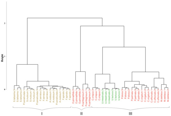
Figure 1.
Hierarchical classification (Bray–Curtis similarity coefficient, Ward’s agglomeration method) of pigment composition samples. Black braces indicate optimal clusters. Colors indicate algae groups: green (Chlorophyta), brown (Ochrophyta), and red (Rhodophyta).
3.2. Raw Reflectance Spectra Analysis
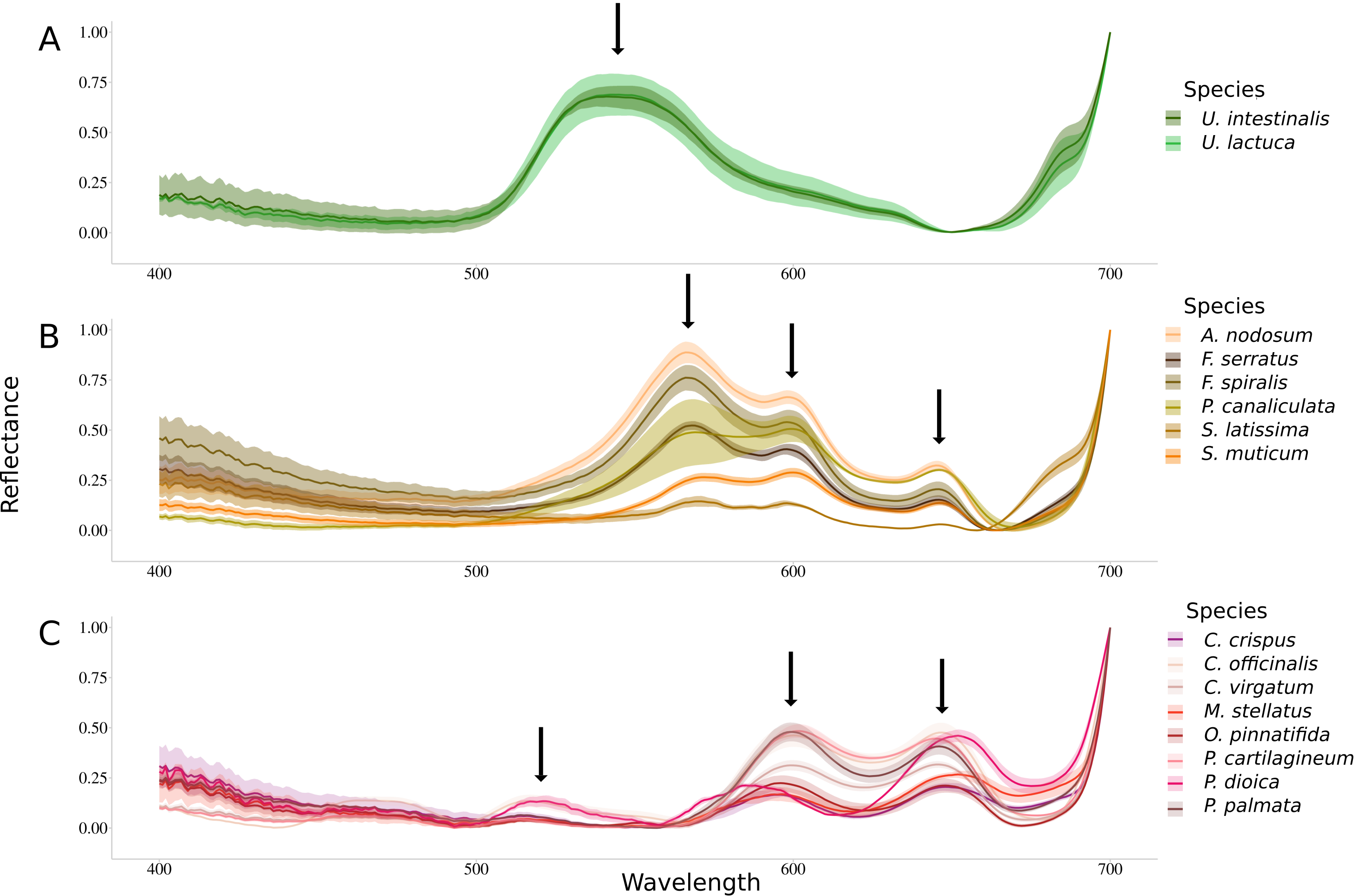
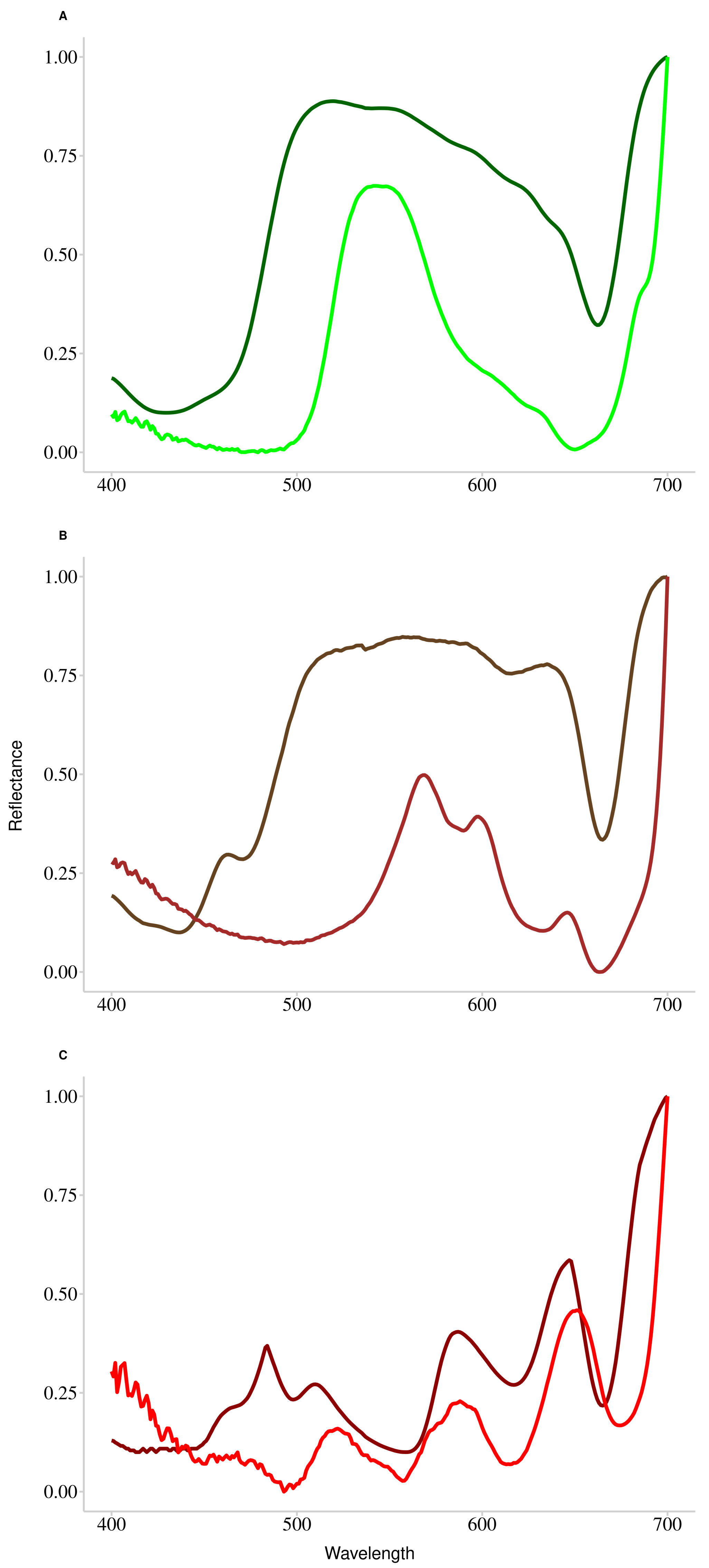
Figure 2 shows spectra of Min-Max normalized reflectance for each species. All species belonging to the same phylum showed a common pattern in their reflectance spectrum. This spectral feature is, in particular, defined by the number of peaks present in the reflectance spectra (identified by black arrows). Green algae are characterized by a large single reflectance peak at 545 nm (Figure 2A). Brown algae showed three reflectance peaks, including a brown algae-specific peak located at 570 nm (Figure 2B). The other two reflectance peaks are also detected in the red algae and are, respectively, located at 600 nm and 645 nm. Red algae are characterized by three reflectance peaks, the two common to brown algae and one specific to this group detected at 515 nm (Figure 2C).
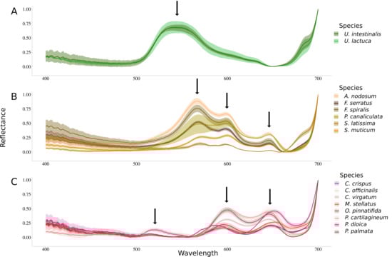
Figure 2.
Normalized reflectance spectra measured for the sixteen species. Dark lines represent the mean while intervals represent the associated standard deviations. Downward arrows indicate local maxima. (A) Chlorophyta species, (B) Ochrophyta species and (C) Rhodophyta species.
3.3. Reflectance Data Classification
All results from this Section 3.3 were obtained on the spectral library consisting of reflectance spectrum measurements acquired on 29 and 30 October 2019 mission. This dataset allowed to compare the classification results obtained with the Euclidean approach and the one developed during this study. Following this, the robustness of the obtained classifications was tested by adding to the initially constituted library, the reflectance measurements acquired on 12 November 2019.
3.3.1. Application of the Euclidean Technique
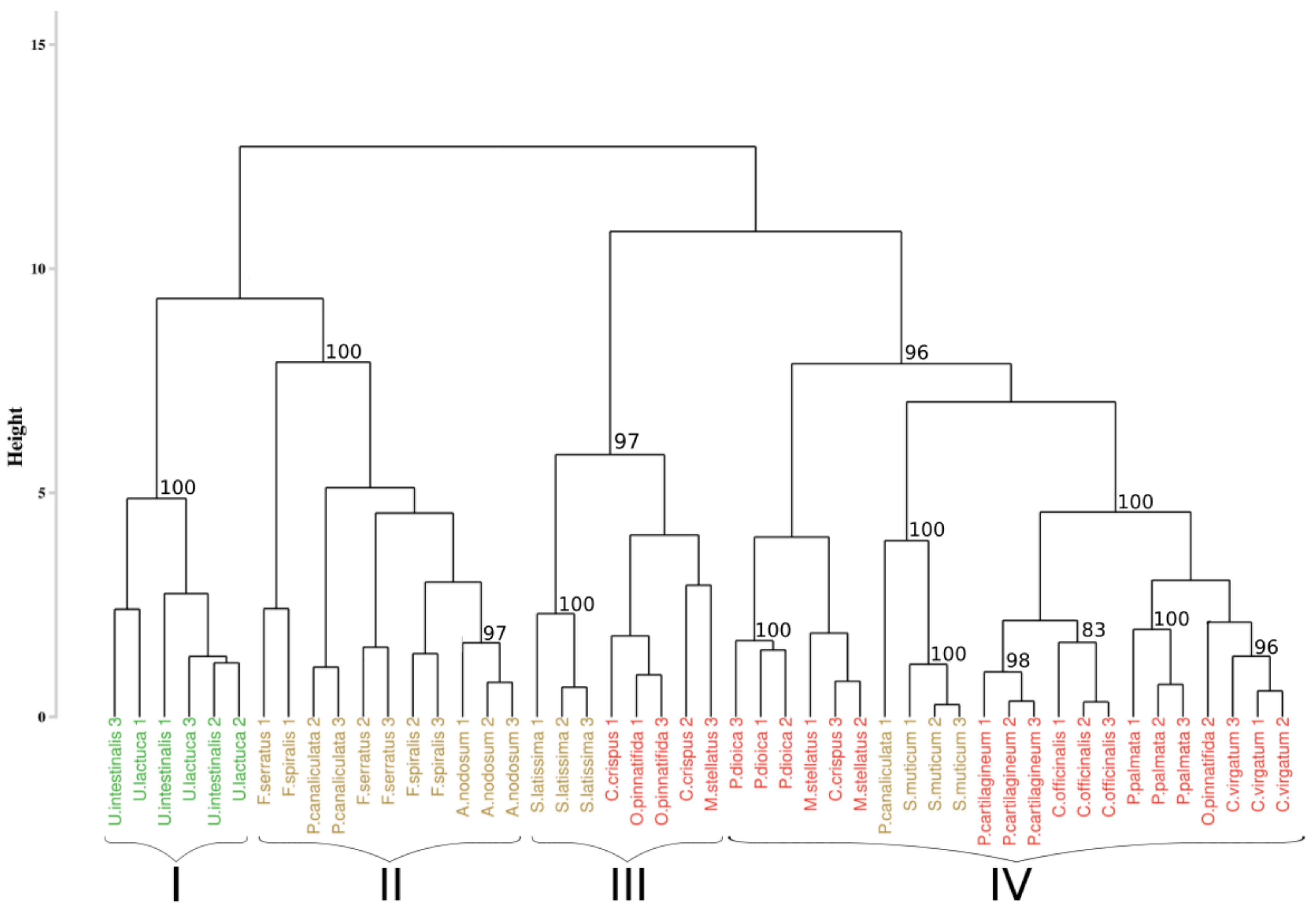
The results of the first approach applied to the hyperspectral library acquired during this study are presented in Figure 3. The analysis of the inter-cluster inertia suggests an optimal number of four clusters. Two clusters were constituted by only one group of algae. The first one (cluster I) gathered all the individuals belonging to the green algae with a bootstrap p-value of 100%, while the second one (cluster II) only concerns brown algae with a 100% p-value. The two others clusters (clusters III and IV) showed a mixture between brown and red algae, with a p-value of 97% and 96%, respectively. However, in both of these clusters, individuals belonging to the same phylum were successfully grouped, which led to the creation of sub-clusters, with a bootstrap p-value of 100% in both case. Focusing on the species-level classification, six species out of the sixteen were correctly discriminated, with a p-value superior to 95%. Concerning Corallina officinalis, a grouping of individuals was observed, with a p-value of 93%.
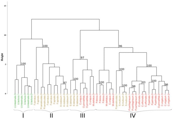
Figure 3.
Dendrogram obtained from cluster analysis of the dissimilarity between the standardized spectra of the sixteen species calculated using the Euclidean distance and a complete linkage, according to the Euclidean approach. Black braces indicate optimal clusters. Colors, used to facilitate visual interpretation, indicate algae groups: green (Chlorophyta), brown (Ochrophyta), and red (Rhodophyta). The value above each node indicate the p-value (%) associated with their bootstrap resampling.
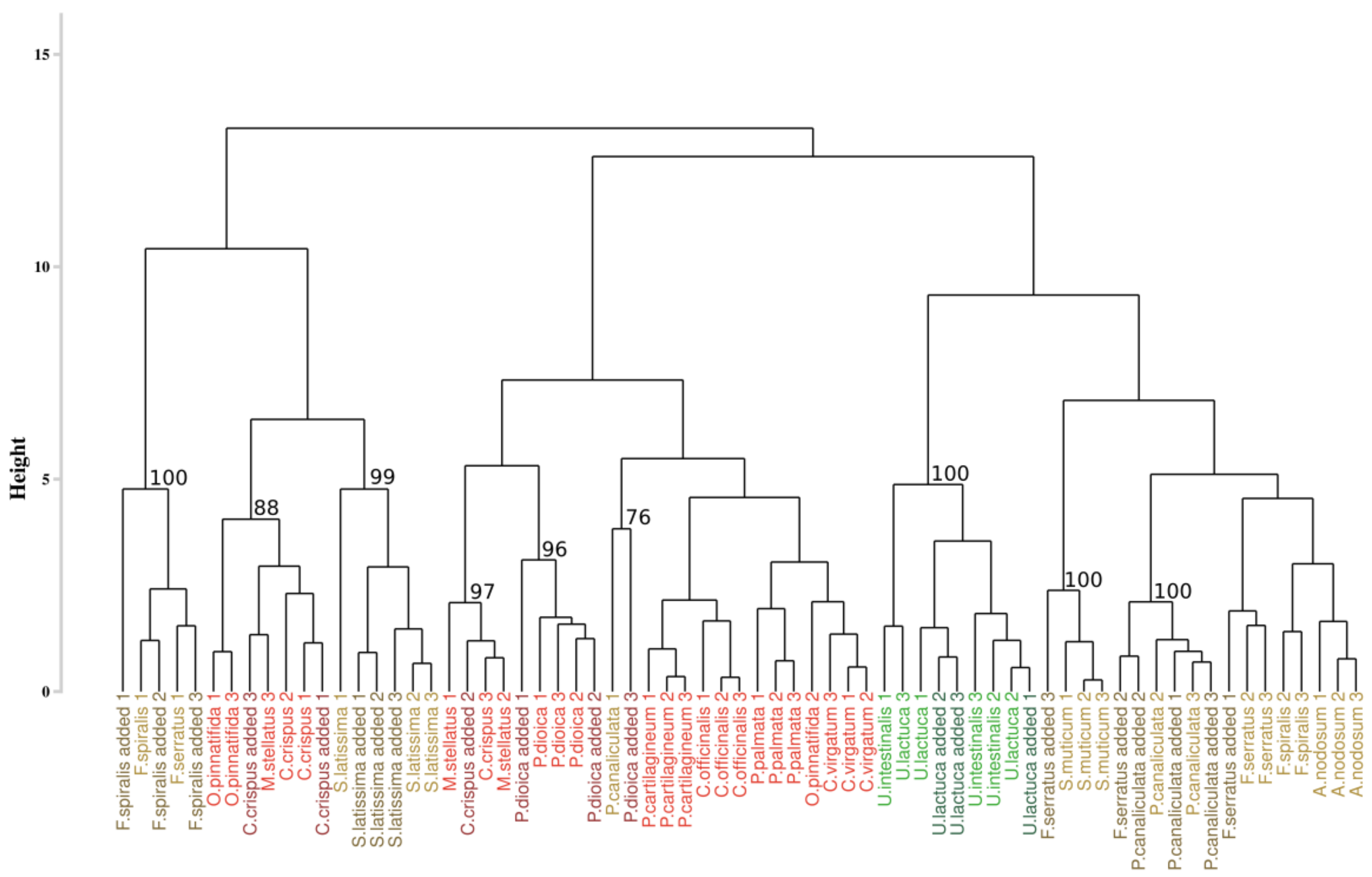
With the intention to test the robustness of this approach, it was applied to a new data set composed of the initial data to which 7 new individuals were added (Figure 4). Among all the additional species, only individuals belonging to Saccharina latissima were gathered with the suitable species, with a bootstrap p-value of 99%. Other individuals were unevenly distributed within the dendrogram, but they were classified with individuals belonging to the same phylum. For example, individuals added of Fucus serratus were grouped with individuals belonging to Pelvetia canaliculata (p-values of 100%) but also with those of Sargassum muticum for one of them (p-values of 100%).

Figure 4.
Dendrogram obtained from the addition of the supplementary individuals and from the Euclidean approach. The dissimilarity matrix was computed with the Euclidean distance and the complete linkage. Colors, used to facilitate visual interpretation, indicate algae groups: green (Chlorophyta), brown (Ochrophyta) and red (Rhodophyta). Names in dark colors show the added individuals. The value above each node indicate the p-value (%) associated with their bootstrap resampling.
The first approach applied to our dataset may thus not be resilient to the addition of new individuals.
3.3.2. Application of the Spectral Angle Mapper Approach
Figure 5 represents the results of the HCA performed on the first-derivative applied to the Min-Max normalized reflectance data. After inertia analysis, the optimal partitioning of the reflectance data was set to four clusters. Results of the partitioning showed clusters composed of individuals belonging to the same phylum, with green algae grouped (cluster I) with a bootstrap p-value of 100%, brown algae grouped (cluster II) in 91% of the sampling distribution, and the red ones divided into two clusters (clusters III and IV), with a p-value of 100% and 95%, respectively. Classification of individuals also showed a gathering by species for eleven species on the sixteen studied, with a bootstrap p-value higher than 94%, except for individuals belonging to Fucus species. Indeed, in this case, the associated p-value was 86% for Fucus serratus and 89% for Fucus spiralis. However, when considering the group formed by Fucus species, the p-value was higher (90%). For the five remaining species, individuals from the same species were generally close to each other.
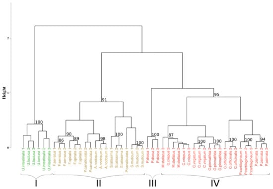
Figure 5.
Dendrogram resulting from HCA applied on the sixteen species. Distance matrix was calculated using the SAM algorithm applied on the 1st derivative data. Black braces indicate optimal clusters. Colors, used to facilitate visual interpretation, indicate algae groups: green (Chlorophyta), brown (Ochrophyta), and red (Rhodophyta). The value above each node indicate the p-value (%) associated with their bootstrap resampling.
The addition of new individuals slightly modified the composition of the original clusters by classifying Saccharina latissima individuals within the red algae cluster (Figure 6). Despite this mixture, all the individuals belonging to Saccharina latissima were successfully grouped in the same sub-cluster that was isolated from the red algae species, 100% of the sampling distribution. Consequently, there was no mixture between species from different phyla meaning that the assessment of the robustness of proposed approach is consistent with the addition of supplementary individuals. On the 7 added individuals, only three were classified with the species cluster that they belong to (i.e., Porphyra dioica with a p-value of 100%, Saccharina latissima with a p-value of 100% and Pelvetia canaliculata with a p-value of 96%). Remaining species were classified in the appropriate phylum, but they are unevenly distributed among different species. Among all the species, nine species from the sixteen were well-classified. Even if this approach is more resilient to individuals species addition, only half of the added individuals were well-classified.
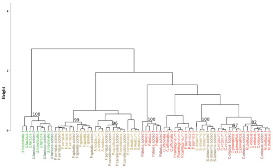
Figure 6.
Dendrogram obtained from the addition of the supplementary individuals and from the developed approach. The dissimilarity matrix was computed with the SAM algorithm and Ward’s agglomeration. Colors, used to facilitate visual interpretation, indicate algae groups: green (Chlorophyta), brown (Ochrophyta) and red (Rhodophyta). Names in dark colors show the added individuals. The value above each node indicate the p-value (%) associated with their bootstrap resampling.
Comparison of the dendograms from the two approaches was performed using Cohen’s Kappa coefficient. In the case of the initial dendrogram, composed only of individuals from the first sampling event (29 and 30 October 2019), the result of the comparison was 0.687. This means that the two dendrograms had more than 31% differences. The addition of new individuals further accentuated this difference. Indeed, the coefficient obtained was 0.619, which corresponds to a difference between the dendrograms of more than 38%.
3.4. Assessment of the Approaches Reproducibility over Time
The assessment of the approaches reproducibility over time was performed on the data from the monthly monitoring, acquired between September 2019 and September 2020.
3.4.1. Application of the Euclidean Technique
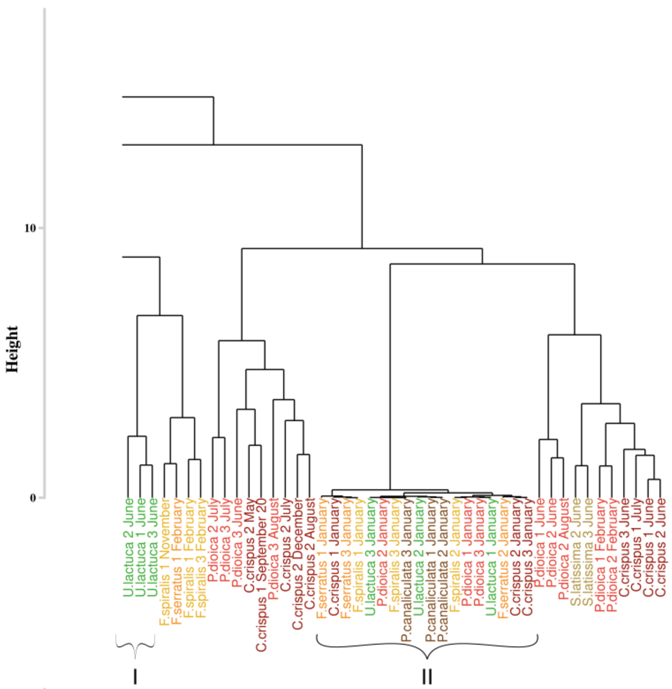
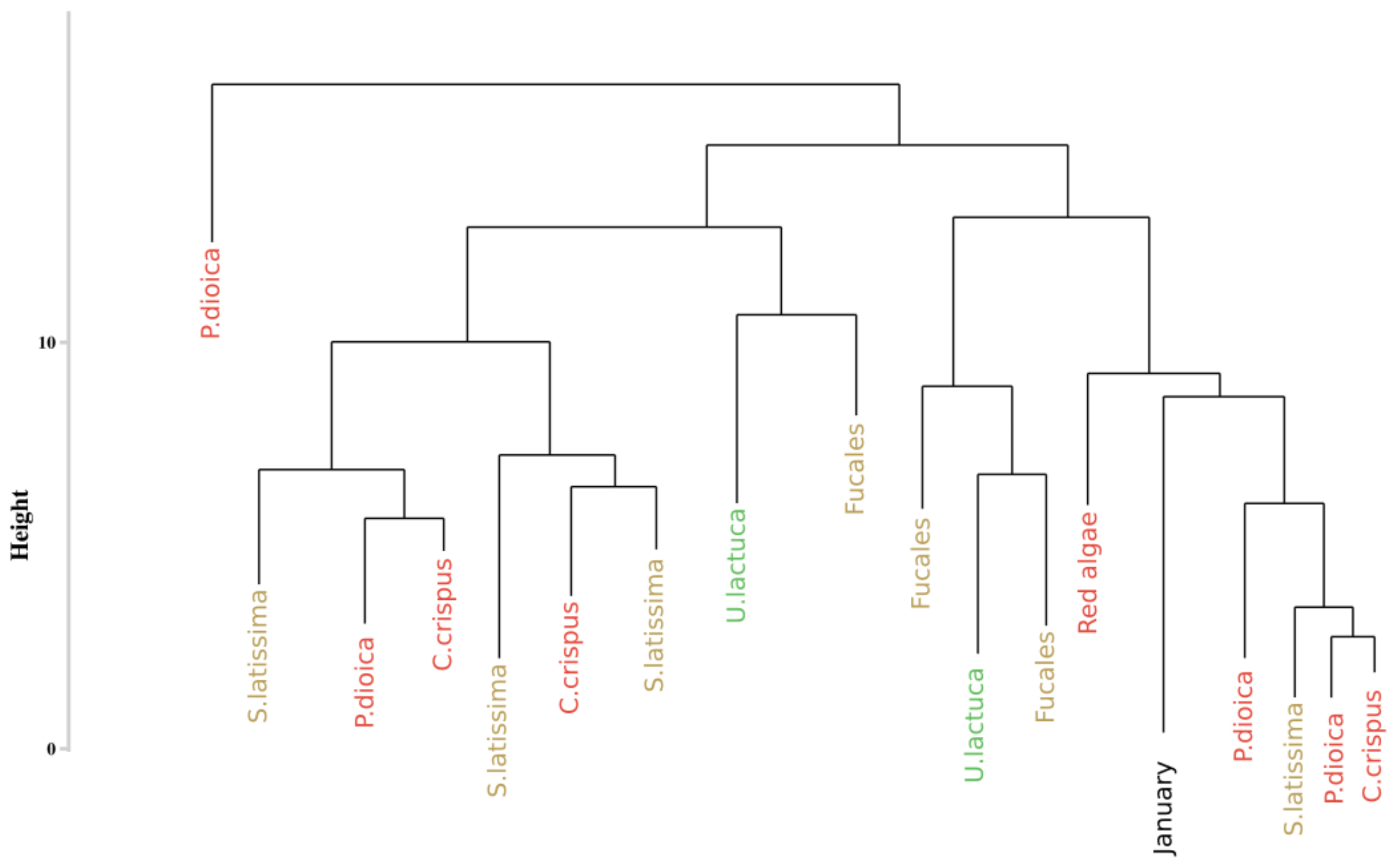
An extract of the dendrogram (chosen as the most mixed part) resulting from the classification approach of Olmedo-Masat et al. [27] applied on the reflectance data acquired during the monthly monitoring is presented on Figure 7. The obtained results displayed a classification linked to the month of sampling for some clusters. Indeed, at the left of the dendrogram (cluster I, in green), a group composed of Ulva lactuca sampled in June appears. This monthly merging is particularly visible within cluster II, which gathers all species sampled in January. However, this monthly merging can not be extended to the whole dendrogram. To facilitate the reading of the dendrogram results, a summary figure is proposed as Figure 8 for clarity. This synoptic representation of the whole dendrogram showed an important mixture of the individuals, whatever the phylum or the species within the dendrogram. For example, Saccharina latissima individuals are separated into four different groups scattered on the entire dendrogram. The same pattern can be observed for all the species. Concerning the Fucales (Fucus serratus, Fucus spiralis, and Pelvetia canaliculata), the species are mixed and are separated into three different clusters. Following this approach, no clear classification can be extracted using data from the monthly monitoring by using the Olmedo-Masat’s approach.

Figure 7.
Extract of the dendrogram resulting from HCA of the dissimilarity between the standardized spectra of the monthly monitoring data. Dissimilarity was calculated using the Euclidean distance. Colors, used to facilitate visual interpretation, indicate algae groups: green (Chlorophyta), brown (Ochrophyta) and red (Rhodophyta). Variation in the color intensity makes it easier to visually identify the different species of algae. The complete figure is available in Appendix A (Figure A1).
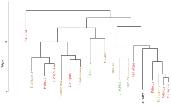
Figure 8.
Simplification of the dendrogram obtained from the HCA of the monthly monitoring data with the Euclidean distance to compute dissimilarity matrix. Colors, used to facilitate visual interpretation, indicate algae groups: green (Chlorophyta), brown (Ochrophyta) and red (Rhodophyta).
3.4.2. Application of the Spectral Angle Mapper Approach
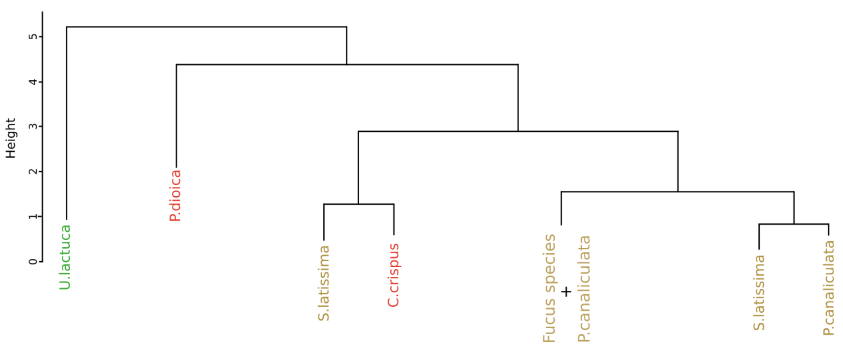
Figure 9 displays the result of the classification performed on the monthly monitoring data with the use of the SAM algorithm, applied on the first derivative data, and to compute the dissimilarity matrix. The part of the dendrogram presented is an extract of the complete dendrogram with the selection of the part which exhibited the greatest variability. Contrary to the result obtained with the approach proposed by Olmedo-Masat et al. [27], the proposed approach based on the SAM algorithm exhibited less heterogeneity in the composition of the groups. In the presented part of the dendrogram, two clusters were detected. The first one, in red, comprised only the individuals belonging to Chondrus crispus. The second one, in brown, consisted in a gathering of different species. These species are Fucus serratus, Fucus spiralis and Pelvetia canaliculata and no classification pattern could be extracted from this cluster. To facilitate the reading of the dendrogram results, a summary figure is proposed as Figure 10 for clarity. Except for the mixed groups of the three Fucales species previously presented, all the clusters are composed of individuals from single species, exhibiting seven clusters in total. Three of them gathered all the individuals belonging to the same species. These clusters are composed of the green algae Ulva lactuca and the two red algae Porphyra dioica and Chondrus crispus. Two clusters are characterized by individuals belonging to Saccharina latissima. Moreover, all the Saccharina latissima individuals are located within these two clusters. The Pelvetia canaliculata cluster located at the right of the dendrogram gathered most of the Pelvetia canaliculata individuals. Finally, Fucus spiralis and Fucus serratus individuals, as well as the six individuals of Pelvetia canaliculata not classified with the other individuals of the same species, are gathered within the Fucales cluster. Comparison of the clusters obtained by the two different approaches yielded a Cohen’s Kappa coefficient of 0.405, which means that the two dendrograms had more than 59% difference between them.
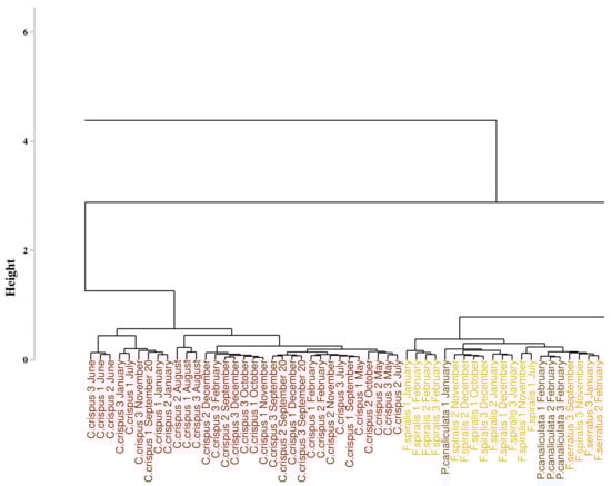
Figure 9.
Extract of the dendrogram obtained from HCA of the dissimilarity between the first derivative reflectance data of the monthly monitoring. Dissimilarity was calculated using the proposed approach which use spectral angle mapper algorithm. Colors, used to facilitate visual interpretation, indicate algae groups: green (Chlorophyta), brown (Ochrophyta), and red (Rhodophyta). Variation in the color intensity makes it easier to visually identify the different species of algae. The complete figure is available in Appendix A (Figure A2).
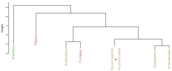
Figure 10.
Simplification of the dendrogram obtained from the HCA of the monthly monitoring data with the SAM algorithm to compute dissimilarity matrix. Colors, used to facilitate visual interpretation, indicate algae groups: green (Chlorophyta), brown (Ochrophyta) and red (Rhodophyta).
4. Discussion
The mapping of macroalgae from hyperspectral imagery requires the development of efficient identification methods that are reproducible to intra-species variation. The approach herein described offers a new and efficient procedure for the identification of species using the HCA technique. Based on the use of the spectral angle mapper algorithm applied to the first derivative of the normalized data, this new approach allowed the majority of the species studied to be efficiently discriminated, regardless of the considered season.
4.1. Macroalgae Discrimination
4.1.1. Pigment
First of all, knowing that the hyperspectral signature depends essentially on pigments, the pigment contents were analyzed to see if it was possible to differentiate the species according to this characteristic. The results of the pigment characteristics obtained showed the existence of specific pigment to each phylum. In particular, chlorophyll b and neoxanthin are pigments specific to Chlorophyta with an absorption around 650 nm [65]. The Ochrophyta are differentiated by the presence of two specific pigments, chlorophyll c (636 nm) and fucoxanthin (550 nm), while Rhodophyta are characterized by the presence of phycoerythrin (563 nm) and phycocyanin (620 nm). With the exception of Pelvetia canaliculata, the results showed a perfect classification at the species level probably explained by the difference in pigment ratios. In the case of Pelvetia canaliculata, the great variability in pigment content between individuals may explain such a bias in the classification obtained. It has been shown by Casal et al. [66] that photosynthetic pigments and accessory pigments partly explain the unique spectral shape of the different phyla and that this spectral shape depends on pigment concentration. This feature reinforces the value of using a hyperspectral library and distance matrix calculation to perform macroalgal classification. However, it has been shown that, in macroalgae, the relationship between pigment content and light absorption may be limited, especially due to the effect of multiple scattering: [67,68,69]. In order to understand such differences between light absorption and pigment content, a complementary analysis was performed on three characteristic species of each phylum. From the absorbance of the pigments, obtained by spectroscopic analysis, the reflectance was evaluated using the formula , allowing the comparison between the reflectance of the whole individual and the reflectance reconstructed from the total pigment content alone. Figure 11 shows the results of the overlapping of the normalized curves obtained from the measurement of the reflectance (in light colors) and the reconstructed reflectance (in dark colors). With this additional information, substantial spectral differences between the two curves were systematically observed, explained by two phenomena. The first one, mainly observable in green and brown algae, is a difference in the width of the reflectance peak between the two curves. Indeed, the width of the reflectance peak based on absorbance data is wider than that based on measured reflectance data. This difference can be explained by the presence of other molecules with absorption properties in the living material that are not present in the extract. These molecules, which are non-photosynthetic tissues (i.e., proteins or nucleic acids), have an impact on light absorption, especially in the blue light region (wavelengths below 500 nm or Soret bands). The second phenomenon is a shift, of a few nm, of each wavelength value of the reflectance minima (comparable to the absorption maximum). These shifts may be due to the extraction procedure, which may alter the protein-pigment complexes and the spatial conformation of the proteins, thus modifying the optical properties of the sample. Despite the information provided by this analysis, the reflectance data obtained using this equation should be treated with caution due to the difference in reflectance properties between the living material and the extract. In order to consider only the pigments effects on the classification, it would be interesting to assign a maximum absorption wavelength to each pigment. Such work has already been done by Méléder et al. [70] to estimate the pigment composition in vivo for microphytobenthos, with promising results. However, the cellular complexity of macroalgae makes such estimation more complicated. In particular, it appears that in macroalgae, pigment uptake characteristics may vary from one phyla to another, but also within the same phyla [71]. In plants, a similar conclusion was made by Huang et al. [72], who concluded that remote quantification of pigments is not very efficient, despite a good knowledge of the pigment absorption regions.
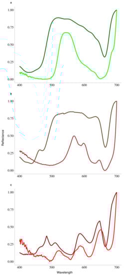
Figure 11.
Superposition of the normalized reflectance spectra acquired from the ASD measurements (in light color) and the normalized reflectance spectra reconstructed from the logarithmic transformation of absorbance measured in laboratory conditions (in dark color). (A) Chlorophyta species, (B) Ochrophyta species and (C) Rhodophyta species.
4.1.2. Spectral Signatures Classification
To investigate the effectiveness of using hyperspectral data for macroalgal discrimination, the recently published approach of Olmedo-Masat et al. [27] was used. Despite their promising results, this procedure proved not to be suitable for the discrimination of species acquired on the rocky coast of the English Channel. Indeed, the results showed that this approach did not allow to correctly group individuals belonging to the same phylum. Red algae were always mixed with brown algae, and no real differentiation between these two phyla could be obtained. The difference with the results obtained by Olmedo-Masat et al. [27] is mainly explained by the preprocessing applied to the data, and in particular the way individuals of the same species were considered. In their analysis, all individuals of the same species were grouped before classification, and intraspecific variation was not considered. By considering only the mean of individuals belonging to the same species (or by extension the median, as was done by Olmedo-Masat et al. [27]), the differences observed between the reflectance curves of each species are highlighted (Figure 2). In contrast, when considering the variability within each species, this difference is strongly reduced, with a greater overlap between the reflectance curves of the different species. The previous results show that the use of a classification based on reflectance values, as done by [27] is not suitable for accurate discrimination of hyperspectral macroalgal reflectance data. The procedure developed in this study is based on the use of the algorithm SAM and focuses on the study of the spectral shape. This allows to reduce the effects of the intraspecific variability, expressed mainly through the variation of the signal intensity, without consequent modification of the spectral shape. Indeed, intraspecific variations are generally related to a difference in the composition of individuals (pigment content, chloroplast density, cell or tissue arrangement), which is a response to environmental conditions, such as light availability, or related to the developmental stage of individuals: [73,74,75], by playing on reflectance values. The results obtained following the use of the developed approach, on the hyperspectral library of macroalgae, revealed an appropriate grouping of individuals according to the phylum to which they belong. Such discrimination of the three main macroalgal groups was also demonstrated by Chao Rodríguez et al. [47] with three different methods (RGB colorimetry, true skill statistics optimal band (TSS-OB), and derived spectroscopy). However, they concluded the inability to discriminate individuals at a higher level (i.e., than the species level). In the present study, the classification performed on the macroalgal spectral library, with the SAM algorithm applied on the first derivative hyperspectral reflectance data, demonstrated, for the first time, the possibility of reaching the species level for most of the studied species, considering the intraspecific variability. For misclassified species, the spectral shape similarities are systematically very important. For Ulva sp., the strong similarity between reflectance spectra explains these discrimination difficulties (less than 9% difference on average with a maximum at 68%). This strong similarity is explained by a content and a pigmentary structure quite identical in the two species. The same phenomenon occurred between Mastocarpus stellatus and Chondrus crispus. Figure 2C, but in this case, the similarity concerns only the shape of the two curves. This similarity is reflected in the calculation of SAM which shows on average 0.10% difference with a maximum of 0.14%. Since the distance SAM is based on the spectral shape, and more precisely on the angle calculated between different spectra, the differentiation of two similar spectral curves is not possible even if they present differences in terms of reflectance values as it is the case for Mastocarpus stellatus and Chondrus crispus. Obviously, the classification resulting from using the SAM algorithm to compute the distance matrix on the data derived at the first order performed better and is more suitable for our study area.
4.2. Robustness
In order to validate the effectiveness of the developed procedure, a robustness assessment was performed, adding additional individuals to the initial dataset, and applying both approaches to the new dataset. In both cases, this addition led to the modification of the dendrogram, with a lesser impact on the dendrogram based on the SAM. Indeed, in this case, only one species of brown algae migrated within the red algae cluster, whereas with the Olmedo-Masat approach, the addition of new individuals generated the formation of three new clusters. In both cases, these changes in the dendrograms denote a change in the distance matrix, with two species belonging to different phyla being classified together. As the experiment was performed under controlled conditions and on similar living material, this variation could be related to the modification of the pigment content of the species linked to environmental conditions. Indeed, in macroalgae, as in most photosynthetic organisms, protective mechanisms involving pigments are put in place to protect macroalgae from stresses induced by environmental conditions. In particular, variations in light intensity strongly impact photosynthetic pigments by modifying their quantity but also the pigment composition [76,77]. In the present study, this effect is mainly visible for violaxanthin, involved in the xanthophyll cycle. This cycle is one of the main defense mechanisms against high light intensities [78,79]. Despite the classification errors, with the procedure developed in this study, individuals belonging to the same phylum are always grouped together which is not the case for the Olmedo-Masat approach. Using the procedure developed in this study, only individuals from the red algae phylum form an isolated cluster. This is explained by the low reflectance values (lower than 0.15) observed for the individuals of this species. Indeed, these low values mask the general spectral shape and the spectral shape related to this species is then found to be close to that of the red algae species with almost no difference between the peaks at 570 nm and 600 nm and a slight peak at 645 nm. (Figure 2). Furthermore, because the results of the SAM calculation showed very little difference between species (less than 0.1%) as well as between phyla (less than 2%), the addition of new Saccharina latissima species brought the Saccharina latissima cluster closer to red algae. Despite this phenomenon, all individuals of Saccharina latissima remained close to each other.
4.3. Monthly Monitoring
The results obtained for the discrimination of species show that for a given period, the approach developed allows an efficient classification of individuals, contrary to the Olmedo-Masat procedure. However, one of the main interests of the use of the spectral library is not to have to perform field measurements in parallel with the mapping campaigns. To achieve this goal, the classification of the hyperspectral library must be reproducible over time. In order to test this, both approaches were applied on a monthly monitoring of macroalgal reflectance spectra. The results obtained from this comparative analysis showed that the Euclidean method is sensitive to seasonal variations. Indeed, no classification could be extracted from the analysis, and each group of species was distributed along the dendrogram. These results may be related to the seasonal evolution of pigment content in relation to changes in environmental conditions (light and temperature); [77,80]. Similar results have been demonstrated in terrestrial [81] and marine [49] environments, with significant seasonal effects on the reflectance properties of the materials studied. More recently, Selvaraj et al. [82] have demonstrated that, in algae, changes in pigment content due to seasonal variations have a significant impact on the reflectance signal, and mainly in summer when conditions are most stressful. The results obtained by using the developed approach, show an efficient classification whatever the season considered. Indeed, green and red algae species form monospecific groups whatever the sampling month. In the case of brown algae, two groups are formed while three other species are mixed. It is interesting to note that there is no mixing of species belonging to different phyla, unlike the Olmedo-Masat approach. The result obtained with the procedure developed in this study is explained both by the preprocessing applied to the data, as well as by the use of SAM to calculate the distance matrix. Indeed, the succession of these treatments allows to get rid of the effects of the seasonal variations, in particular when it is about the evolution of the quantity of pigments, by considering only the spectral shape. This result allows us to consider the possibility of using a large spectral library composed of reflectance spectra acquired during the year to perform species discrimination in hyperspectral imaging without simultaneous field surveys. These results reinforce the interest of using a spectral library coupled with a hierarchical cluster analysis to perfectly discriminate individuals from hyperspectral imagery.
The different results obtained show the interest of using a spectral library for the discrimination of macroalgae. However, as shown by Chao Rodríguez et al. [47] to reach the level of species with the reflectance data remains theoretical. However, this classification can be improved by considering complementary data, especially topo-bathymetry. Indeed, as mentioned previously, it is well known that macroalgal species have a belt-like organization, specific to a bathymetric level. As in the present study, the mixed species are specific and characteristic of a different belt, the topo-bathymetric information will allow to further discriminate the species. For example, the Fucus serratus are inferred to the coastal zone between the middle and lower intertidal level while the Fucus spiralis are specific to the upper shoreline level. Coupled with this relevant field knowledge, the hyperspectral technique certainly becomes a powerful tool to discriminate macroalgal species with greater accuracy. The in situ use of the approach developed during this study is also conditioned by environmental variations during data acquisition. In particular, variations in light intensity during the acquisition mission can potentially modify the acquired spectral responses. However, the succession of the different treatments used in the procedure developed in this study should allow us to avoid the effects of these variations. One of the obstacles to the precise identification of species in in situ conditions is the presence of species mixing within the different communities. However, the use of hyperspectral cameras on board UAVs allows to increase the spatial resolution of acquisition, up to 2 cm [42]. If this resolution is not sufficient to separate the mixtures, it is possible to use unmixing models. For example, Uhl et al. [83] studied the possibility to unmixed species, thanks to linear unmixing algorithm. They concluded to the possibility to separate mixed species to a limited extend. This feature allows to discriminate mixed species within the dendrogram in order to draw maps as precise as possible to follow the evolution of the different communities.
5. Conclusions
In this study, a new approach to macroalgal discrimination was developed using a library of reflectance spectrum measurements acquired under controlled conditions. This procedure is based on the use of the SAM algorithm, for the first time applied on the first derivative of the reflectance measurement data, and not on the raw data. To our knowledge, this has never been done on reflectance signals acquired on macroalgae. The classification results obtained were compared to those obtained, on the same dataset, with the Olmedo-Masat et al. [27] approach, which is the most successful procedure published to date. The comparison was performed on a spectral library including 16 species and on a monthly monitoring based on 7 species, thus allowing to take into account the robustness of the results to natural variabilities. The results obtained showed that the developed procedure allows a relatively efficient discrimination of species compared to that obtained using the Olmedo-Masat approach, with more than 30% differences between the two approaches. Moreover, this same procedure is also resilient to seasonal variations, which does not seem to be the case for the Olmedo-Masat approach. However, it would be interesting to see if this robustness is maintained between years, and applies to other sites. Indeed, since the conditions between the different seasons are not the same between two consecutive years (e.g., more or less severe winter or summer), variations in the spectral responses are to be expected. Finally, the different steps used in this approach suggest good results when applied to data acquired in real conditions. Indeed, these different steps allow to get rid of the possible variations of the experimental conditions, in particular of the luminosity and the seasonal effects.
Author Contributions
Conceptualization, F.D. and F.G.; Data curation, F.D.; Formal analysis, F.D., F.G. and G.D.; Methodology, F.D. and C.V.; Supervision, F.G., C.V. and N.S.; Writing—original draft, F.D.; Writing—review and editing, F.D., C.V., N.S. and F.G. All authors have read and agreed to the published version of the manuscript.
Funding
F. Douay is funded by a PhD studentship from the Université du Littoral côte d’Opale (ULCO) and the Pôle Metropolitain Côte D’Opale (PMCO).
Acknowledgments
This work has been financially supported by the European Union (ERDF), the French State, the French Region Hauts-de-France and Ifremer, in the framework of the project CPER MARCO 2015-2020. We would like to thank the ULCO University and the CNES TOSCA program for funding the LOG hyperspectral radiometer through the BQR-HYPCOOL and CNES TOSCA funds.
Conflicts of Interest
The authors declare no conflict of interest.
Appendix A
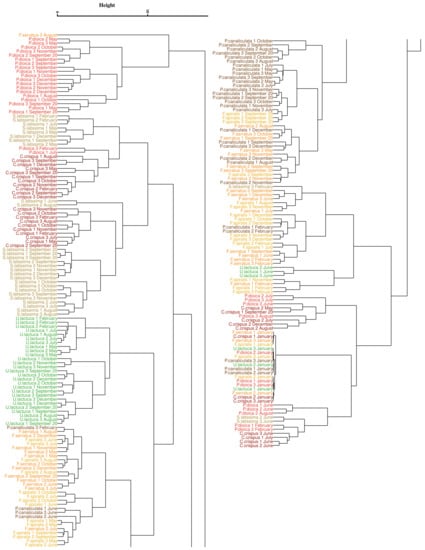
Figure A1.
Dendrogram obtained from HCA of the dissimilarity between the standardized spectra of the monthly monitoring data. Dissimilarity was calculated using the Euclidean distance and a complete linkage. Colors indicate macroalgae groups: green (Chloropĥyta), brown (Ochrophyta) and red (Rhodophyta). Variations in the color intensity makes it easier to visually identify the different species of algae. To facilitate the integration of these results in the paper, the dendrogram has been separated into two parts, the right part being the continuation of the left one.
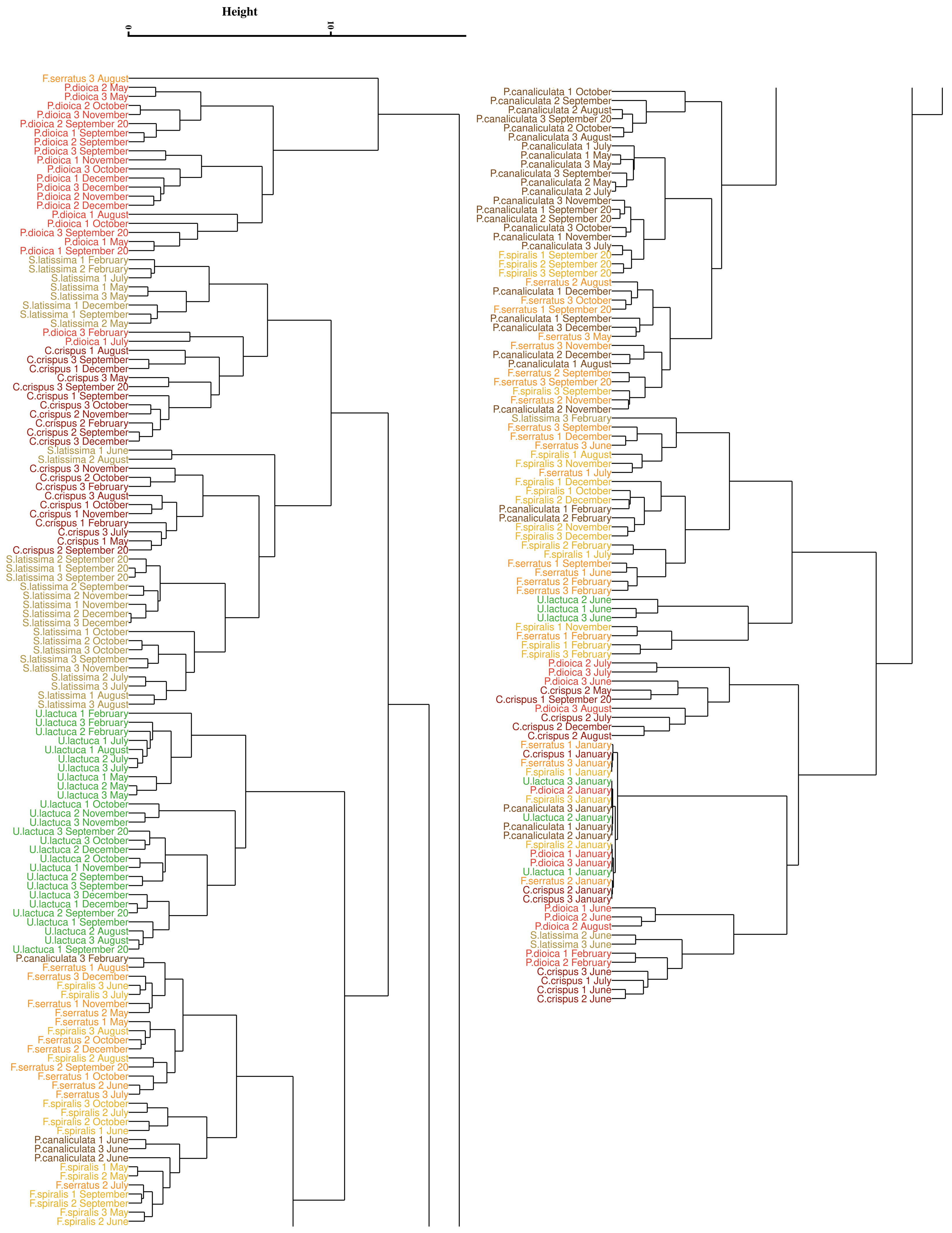

Figure A2.
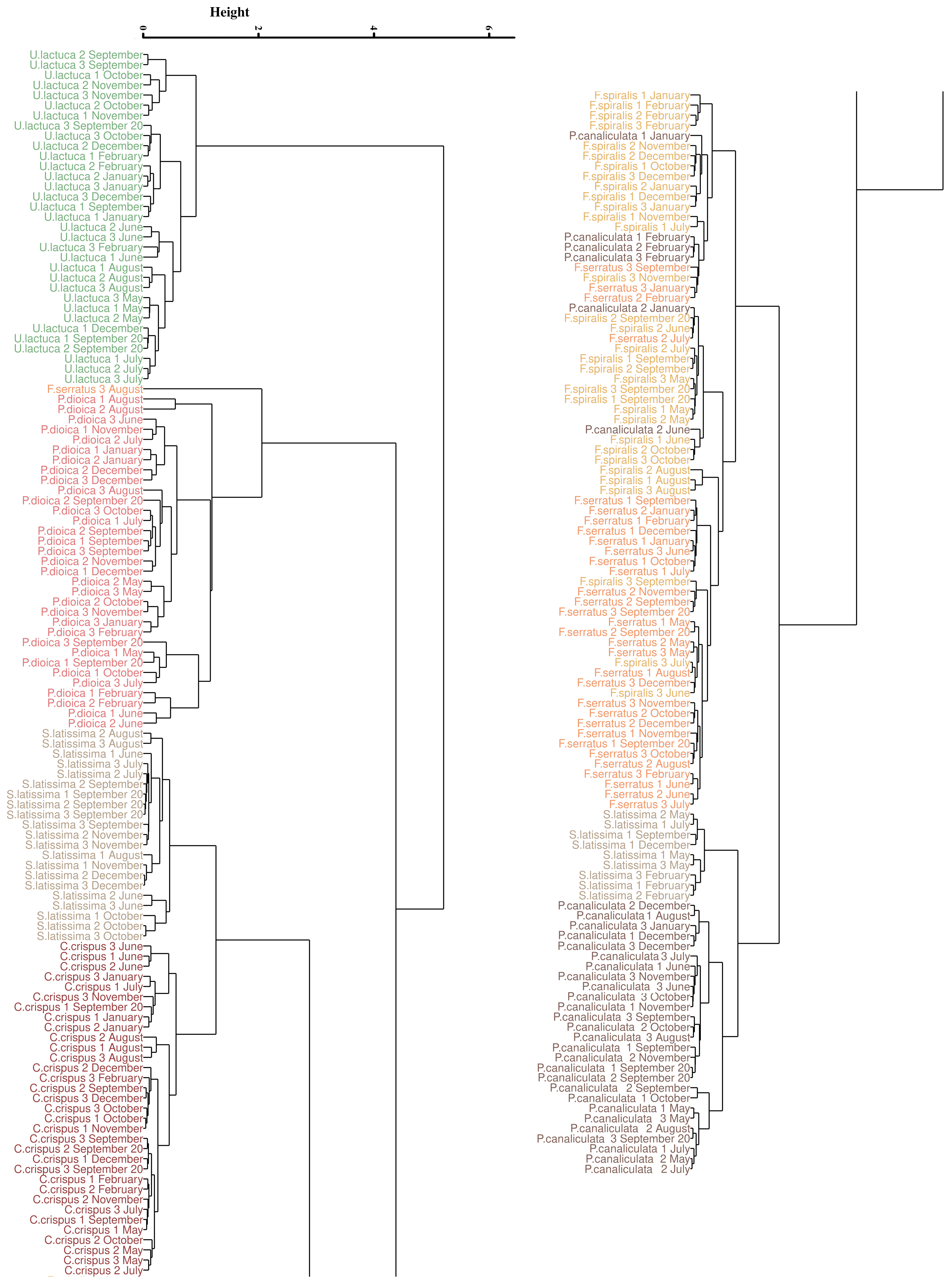
Dendrogram obtained from HCA of the dissimilarity between the first derivative data of the monthly monitoring. Dissimilarity was calculated using the proposed approach which use spectral angle mapper algorithm. Colors indicate macroalgae groups: green (Chloropĥyta), brown (Ochrophyta) and red (Rhodophyta). Variations in the color intensity makes it easier to visually identify the different species of algae. To facilitate the integration of these results in the paper, the dendrogram has been separated into two parts, the right part being the continuation of the left one.
Figure A2.
Dendrogram obtained from HCA of the dissimilarity between the first derivative data of the monthly monitoring. Dissimilarity was calculated using the proposed approach which use spectral angle mapper algorithm. Colors indicate macroalgae groups: green (Chloropĥyta), brown (Ochrophyta) and red (Rhodophyta). Variations in the color intensity makes it easier to visually identify the different species of algae. To facilitate the integration of these results in the paper, the dendrogram has been separated into two parts, the right part being the continuation of the left one.
References
- Borg, Å.; Pihl, L.; Wennhage, H. Habitat Choice by Juvenile Cod (Gadus Morhua L.) on Sandy Soit Bottoms with Different Vegetation Types. Helgol. Meeresunters. 1997, 51, 197–212. [Google Scholar] [CrossRef] [Green Version]
- Shaffer, A. Preferential Use of Nearshore Kelp Habitats by Juvenile Salmon and Forage Fish. In Proceedings of the Georgia Basin/Puget Sound Research Conference, Vancouver, BC, Canada, 31 March–3 April 2003. [Google Scholar]
- Lorentsen, S.H.; Grémillet, D.; Nymoen, G.H. Annual Variation in Diet of Breeding Great Cormorants: Does It Reflect Varying Recruitment of Gadoids? Waterbirds 2004, 27, 161–169. [Google Scholar] [CrossRef]
- Buschmann, A. Intertidal Macroalgae as Refuge and Food for Amphipoda in Central Chile. Aquat. Bot. 1990, 36, 237–245. [Google Scholar] [CrossRef]
- Rassweiler, A.; Arkema, K.K.; Reed, D.C.; Zimmerman, R.C.; Brzezinski, M.A. Net Primary Production, Growth, and Standing Crop of Macrocystis Pyrifera Southern California. Ecology 2008, 89, 2068. [Google Scholar] [CrossRef] [PubMed]
- Abdullah, M.I.; Fredriksen, S. Production, Respiration and Exudation of Dissolved Organic Matter by the Kelp LaminariaHyperborea Along West Coast Norway. J. Mar. Biol. Assoc. UK 2004, 84, 887–894. [Google Scholar] [CrossRef]
- Ryther, J.H. Geographic Variations in Productivity. In The Sea: Ideas and Observations on Progress in the Study of the Seas; Hill, M.N., Ed.; Wiley-Interscience: New York, NY, USA, 1963; pp. 347–380. [Google Scholar]
- Tomanek, L.; Helmuth, B. Physiological Ecology of Rocky Intertidal Organisms: A Synergy of Concepts. Integr. Comp. Biol. 2002, 42, 771–775. [Google Scholar] [CrossRef] [PubMed]
- Chappuis, E.; Terradas, M.; Cefalì, M.E.; Mariani, S.; Ballesteros, E. Vertical Zonation Is the Main Distribution Pattern of Littoral Assemblages on Rocky Shores at a Regional Scale. Estuar. Coast. Shelf Sci. 2014, 147, 113–122. [Google Scholar] [CrossRef] [Green Version]
- Raffaelli, D.; Hawkins, S. Intertidal Ecology; Springer: Dordrecht, The Netherlands, 1999. [Google Scholar] [CrossRef]
- Vadas Sr, R.L.; Wright, W.A.; Beal, B.F. Biomass and Productivity of Intertidal Rockweeds (Ascophyllum Nodosum LeJolis) in Cobscook Bay. Northeast. Nat. 2004, 11, 123–142. [Google Scholar] [CrossRef]
- Mann, K.H. Seaweeds: Their Productivity and Strategy for Growth. Science 1973, 182, 975–981. [Google Scholar] [CrossRef] [PubMed]
- Pereira, T.R.; Engelen, A.H.; Pearson, G.A.; Valero, M.; Serrão, E.A. Response of Kelps from Different Latitudes to Consecutive Heat Shock. J. Exp. Mar. Biol. Ecol. 2015, 463, 57–62. [Google Scholar] [CrossRef] [Green Version]
- Wernberg, T.; Russell, B.D.; Thomsen, M.S.; Gurgel, C.F.D.; Bradshaw, C.J.; Poloczanska, E.S.; Connell, S.D. Seaweed Communities in Retreat from Ocean Warming. Curr. Biol. 2011, 21, 1828–1832. [Google Scholar] [CrossRef] [PubMed]
- Raybaud, V.; Beaugrand, G.; Goberville, E.; Delebecq, G.; Destombe, C.; Valero, M.; Davoult, D.; Morin, P.; Gevaert, F. Decline in Kelp in West Europe and Climate. PLoS ONE 2013, 8, e66044. [Google Scholar] [CrossRef] [PubMed] [Green Version]
- Díez, I.; Muguerza, N.; Santolaria, A.; Ganzedo, U.; Gorostiaga, J. Seaweed Assemblage Changes in the Eastern Cantabrian Sea and Their Potential Relationship to Climate Change. Estuar. Coast. Shelf Sci. 2012, 99, 108–120. [Google Scholar] [CrossRef]
- de la Hoz, C.F.; Ramos, E.; Puente, A.; Juanes, J.A. Climate Change Induced Range Shifts in Seaweeds Distributions in Europe. Mar. Environ. Res. 2019, 148, 1–11. [Google Scholar] [CrossRef]
- Straub, S.C.; Wernberg, T.; Thomsen, M.S.; Moore, P.J.; Burrows, M.T.; Harvey, B.P.; Smale, D.A. Resistance, Extinction, and Everything in between—The Diverse Responses of Seaweeds to Marine Heatwaves. Front. Mar. Sci. 2019, 6, 763. [Google Scholar] [CrossRef]
- Araújo, R.M.; Assis, J.; Aguillar, R.; Airoldi, L.; Bárbara, I.; Bartsch, I.; Bekkby, T.; Christie, H.; Davoult, D.; Derrien-Courtel, S.; et al. Status, Trends and Drivers of Kelp Forests in Europe: An Expert Assessment. Biodivers. Conserv. 2016, 25, 1319–1348. [Google Scholar] [CrossRef] [Green Version]
- Christie, H.; Andersen, G.S.; Bekkby, T.; Fagerli, C.W.; Gitmark, J.K.; Gundersen, H.; Rinde, E. Shifts Between Sugar Kelp and Turf Algae in Norway: Regime Shifts or Fluctuations Between Different Opportunistic Seaweed Species? Front. Mar. Sci. 2019, 6, 72. [Google Scholar] [CrossRef] [Green Version]
- Connell, S.; Foster, M.; Airoldi, L. What Are Algal Turfs? Towards a Better Description of Turfs. Mar. Ecol. Prog. Ser. 2014, 495, 299–307. [Google Scholar] [CrossRef] [Green Version]
- Filbee-Dexter, K.; Wernberg, T. Rise of Turfs: A New Battlefront for Globally Declining Kelp Forests. BioScience 2018, 68, 64–76. [Google Scholar] [CrossRef] [Green Version]
- Coelho, S.M.; Rijstenbil, J.W.; Brown, M.T. Impacts of Anthropogenic Stresses on the Early Development Stages of Seaweeds. J. Aquat. Ecosyst. Stress Recovery 2000, 7, 317–333. [Google Scholar] [CrossRef]
- Hiscock, K.; Southward, A.; Tittley, I.; Hawkins, S. Effects of Changing Temperature on Benthic Marine Life in Britain and Ireland. Aquat. Conserv. Mar. Freshw. Ecosyst. 2004, 14, 333–362. [Google Scholar] [CrossRef]
- Bajjouk, T.; Guillaumont, B.; Populus, J. Application of Airborne Imaging Spectrometry System Data to Intertidal Seaweed Classification and Mapping. Hydrobiologia 1996, 326/327, 463–471. [Google Scholar] [CrossRef]
- Nijland, W. Satellite Remote Sensing of Canopy-Forming Kelp on a Complex Coastline: A Novel Procedure Using the Landsat Image Archive. Remote Sens. Environ. 2019, 220, 41–50. [Google Scholar] [CrossRef]
- Olmedo-Masat, O.M.; Raffo, M.P.; Rodríguez-Pérez, D.; Arijón, M.; Sánchez-Carnero, N. How Far Can We Classify Macroalgae Remotely? An Example Using a New Spectral Library of Species from the South West Atlantic (Argentine Patagonia). Remote Sens. 2020, 12, 3870. [Google Scholar] [CrossRef]
- Nelson, S.A.; Cheruvelil, K.S.; Soranno, P.A. Satellite Remote Sensing of Freshwater Macrophytes and the Influence of Water Clarity. Aquat. Bot. 2006, 85, 289–298. [Google Scholar] [CrossRef]
- Malthus, T.J.; Georgeb, D.G. Airborne Remote Sensing of Macrophytes in Cefni Reservoir, Anglesey, UK. Aquat. Bot. 1997, 58, 317–332. [Google Scholar] [CrossRef]
- Jensen, J.R.; Hodgson, M.E.; Christensen, E. Remote Sensing Inland Wetlands: A Multispectral Approach. Photogramm. Eng. Remote Sens. 1986, 52, 87–100. [Google Scholar]
- Hochberg, E.J.; Atkinson, M.J. Capabilities of Remote Sensors to Classify Coral, Algae, and Sand as Pure and Mixed Spectra. Remote Sens. Environ. 2003, 85, 174–189. [Google Scholar] [CrossRef]
- Karpouzli, E.; Malthus, T.J.; Place, C.J. Hyperspectral Discrimination of Coral Reef Benthic Communities in the Western Caribbean. Coral Reefs 2004, 23, 141–151. [Google Scholar] [CrossRef]
- Kutser, T.; Dekker, A.G.; Skirving, W. Modeling Spectral Discrimination of Great Barrier Reef Benthic Communities by Remote Sensing Instruments. Limnol. Oceanogr. 2003, 48, 497–510. [Google Scholar] [CrossRef] [Green Version]
- Meinesz, A. Methods for Identifying and Tracking Seaweed Invasions. Bot. Mar. 2007, 50, 373–384. [Google Scholar] [CrossRef]
- Uhl, F.; Bartsch, I.; Oppelt, N. Submerged Kelp Detection with Hyperspectral Data. Remote Sens. 2016, 8, 487. [Google Scholar] [CrossRef] [Green Version]
- Anderson, R.; Rand, A.; Share, A.; Bolton, J. Mapping and Quantifying the South African Kelp Resource. Afr. J. Mar. Sci. 2007, 29, 369–378. [Google Scholar] [CrossRef]
- Stekoll, M.S.; Deysher, L.E.; Hess, M. A Remote Sensing Approach to Estimating Harvestable Kelp Biomass. J. Appl. Phycol. 2006, 18, 323–334. [Google Scholar] [CrossRef]
- Schroeder, S.B.; Boyer, L.; Juanes, F.; Costa, M. Spatial and Temporal Persistence of Nearshore Kelp Beds on the West Coast of British Columbia, Canada Using Satellite Remote Sensing. Remote Sens. Ecol. Conserv. 2020, 6, 327–343. [Google Scholar] [CrossRef] [Green Version]
- Manfreda, S.; McCabe, M.; Miller, P.; Lucas, R.; Pajuelo Madrigal, V.; Mallinis, G.; Ben Dor, E.; Helman, D.; Estes, L.; Ciraolo, G.; et al. On the Use of Unmanned Aerial Systems for Environmental Monitoring. Remote Sens. 2018, 10, 641. [Google Scholar] [CrossRef] [Green Version]
- Anderson, K.; Gaston, K.J. Lightweight Unmanned Aerial Vehicles Will Revolutionize Spatial Ecology. Front. Ecol. Environ. 2013, 11, 138–146. [Google Scholar] [CrossRef] [Green Version]
- Rossiter, T.; Furey, T.; McCarthy, T.; Stengel, D.B. UAV-Mounted Hyperspectral Mapping of Intertidal Macroalgae. Estuar. Coast. Shelf Sci. 2020, 242, 106789. [Google Scholar] [CrossRef]
- Kislik, C.; Genzoli, L.; Lyons, A.; Kelly, M. Application of UAV Imagery to Detect and Quantify Submerged Filamentous Algae and Rooted Macrophytes in a Non-Wadeable River. Remote Sens. 2020, 12, 3332. [Google Scholar] [CrossRef]
- Kotta, J.; Remm, K.; Vahtmäe, E.; Kutser, T.; Orav-Kotta, H. In-Air Spectral Signatures of the Baltic Sea Macrophytes and Their Statistical Separability. J. Appl. Remote Sens. 2014, 8, 083634. [Google Scholar] [CrossRef] [Green Version]
- Kutser, T.; Vahtmäe, E.; Metsamaa, L. Spectral Library of Macroalgae and Benthic Substrates in Estonian Coastal Waters. Proc. Est. Acad. Sci. Biol. Ecol. 2006, 55, 329–340. [Google Scholar] [CrossRef]
- Kutser, T.; Vahtmäe, E.; Martin, G. Assessing Suitability of Multispectral Satellites for Mapping Benthic Macroalgal Cover in Turbid Coastal Waters by Means of Model Simulations. Estuar. Coast. Shelf Sci. 2006, 67, 521–529. [Google Scholar] [CrossRef]
- Vahtmäe, E.; Kutser, T.; Martin, G.; Kotta, J. Feasibility of Hyperspectral Remote Sensing for Mapping Benthic Macroalgal Cover in Turbid Coastal Waters—A Baltic Sea Case Study. Remote Sens. Environ. 2006, 101, 342–351. [Google Scholar] [CrossRef]
- Chao Rodríguez, Y.; Domínguez Gómez, J.; Sánchez-Carnero, N.; Rodríguez-Pérez, D. A Comparison of Spectral Macroalgae Taxa Separability Methods Using an Extensive Spectral Library. Algal Res. 2017, 26, 463–473. [Google Scholar] [CrossRef]
- Lubin, D. Spectral Signatures of Coral Reefs Features from Space. Remote Sens. Environ. 2001, 75, 127–137. [Google Scholar] [CrossRef]
- Fyfe, S.K. Spatial and Temporal Variation in Spectral Reflectance: Are Seagrass Species Spectrally Distinct? Limnol. Oceanogr. 2003, 48, 464–479. [Google Scholar] [CrossRef]
- O’Neill, J.D.; Costa, M.; Sharma, T. Remote Sensing of Shallow Coastal Benthic Substrates: In Situ Spectra and Mapping of Eelgrass (Zostera Marina) in the Gulf Islands National Park Reserve of Canada. Remote Sens. 2011, 3, 975–1005. [Google Scholar] [CrossRef] [Green Version]
- Kisevic, M.; Smailbegovic, A.; Gray, K.T.; Andricevic, R.; Craft, J.D.; Petrov, V.; Brajcic, D.; Dragicevic, I. Spectral Reflectance Profile of Caulerpa Racemosa Var. Cylindracea and Caulerpa Taxifolia in the Adriatic Sea. In Proceedings of the 2011 3rd Workshop on Hyperspectral Image and Signal Processing: Evolution in Remote Sensing (WHISPERS), Lisbon, Portugal, 6–9 June 2011; pp. 1–4. [Google Scholar] [CrossRef] [Green Version]
- Arsalane, W.; Rousseau, B.; Duval, J.C. Influence of the Pool Size of the Xanthophyll Cycle on the Effects of the Light Stress in a Diatom: Competition Betwe’en Photoprotection and Photoinhibition. Photochem. Photobiol. 1994, 60, 237–243. [Google Scholar] [CrossRef]
- Beer, S.; Eshel, A. Determining Phycoerythrin and Phycocyanin Concentrations in Aqueous Crude Extracts of Red Algae. Mar. Freshw. Res. 1985, 36, 785. [Google Scholar] [CrossRef]
- Lv, W.; Wang, X. Overview of Hyperspectral Image Classification. J. Sens. 2020, 2020, 4817234. [Google Scholar] [CrossRef]
- R Development Core Team. A Language and Environment for Statistical Computing: Reference Index; R Foundation for Statistical Computing: Vienna, Austria, 2010. [Google Scholar]
- Suzuki, R.; Shimodaira, H. Pvclust: An R Package for Assessing the Uncertainty in Hiearchical Clustering. Bioinformatics 2006, 22, 1540–1542. [Google Scholar] [CrossRef]
- Murtagh, F.; Legendre, P. Ward’s Hierarchical Agglomerative Clustering Method: Which Algorithms Implement Ward’s Criterion? J. Classif. 2014, 31, 274–295. [Google Scholar] [CrossRef] [Green Version]
- Cao, F.; Yang, Z.; Ren, J.; Jiang, M.; Ling, W.K. Does Normalization Methods Play a Role for Hyperspectral Image Classification? arXiv 2017, arXiv:1710.02939. [Google Scholar]
- Demetriades-Shah, T.H.; Steven, M.D.; Clark, J.A. High Resolution Derivative Spectra in Remote Sensing. Remote Sens. Environ. 1990, 33, 55–64. [Google Scholar] [CrossRef]
- Ruffin, C.; King, R. The Analysis of Hyperspectral Data Using Savitzky-Golay Filtering-Theoretical Basis. 1. In Proceedings of the IEEE 1999 International Geoscience and Remote Sensing Symposium. IGARSS’99 (Cat. No.99CH36293), Hamburg, Germany, 28 June–2 July 1999; Volume 2, pp. 756–758. [Google Scholar] [CrossRef]
- Talsky, G. Higher-Order Derivative Spectrophotometry in Environmental Analytical Chemistry. Int. J. Environ. Anal. Chem. 1983, 14, 81–91. [Google Scholar] [CrossRef]
- Boardman, J. SIPS User’s Guide Spectral Image Processing System, Version 1.2; Center for the Study of Earth from Space: Boulder, CO, USA, 1992. [Google Scholar]
- Kruse, F.A.; Heidebrecht, K.B.; Shapiro, A.T.; Barloon, P.J.; Goetz, A.F.H. The Spectral Image Processing System (SIPS) Interactive Visualization and Analysis of Imaging Spectrometer Data. Remote Sens. Environ. 1993, 44, 145–163. [Google Scholar] [CrossRef]
- Ramirez-Lopez, L.; Stevens, A.; Viscarra Rossel, R.; Lobsez, C.; Wadoux, A.; Breure, T. Resemble: Regression and Similarity Evaluation for Memory-Based Learning in Spectral Chemometrics; R Foundation for Statistical Computing: Vienna, Austria, 2020. [Google Scholar]
- Rowan, K.S. Photosynthetic Pigments of Algae; Cambridge University Press: Cambridge, UK; New York, NY, USA, 1989. [Google Scholar]
- Casal, G.; Sánchez-Carnero, N.; Domínguez-Gómez, J.A.; Kutser, T.; Freire, J. Assessment of AHS (Airborne Hyperspectral Scanner) Sensor to Map Macroalgal Communities on the Ría de Vigo and Ría de Aldán Coast (NW Spain). Mar. Biol. 2012, 159, 1997–2013. [Google Scholar] [CrossRef]
- Ramus, J. A Form-Function Analysis of Photon Capture for Seaweeds. Hydrobiologia 1990, 204/205, 64–71. [Google Scholar] [CrossRef]
- Ramus, J. Seaweed Anatomy and Photosynthetic Performance: The Ecological Significance of Light Guides, Heterogeneous Absorption and Multiple Scatter. J. Phycol. 1978, 14, 352–362. [Google Scholar] [CrossRef]
- Enríquez, S.; Agustí, S.; Duarte, C.M. Light Absorption by Marine Macrophytes. Oecologia 1994, 98, 121–129. [Google Scholar] [CrossRef] [PubMed]
- Méléder, V.; Laviale, M.; Jesus, B.; Mouget, J.L.; Lavaud, J.; Kazemipour, F.; Launeau, P.; Barillé, L. In Vivo Estimation of Pigment Composition and Optical Absorption Cross-Section by Spectroradiometry in Four Aquatic Photosynthetic Micro-Organisms. J. Photochem. Photobiol. B Biol. 2013, 129, 115–124. [Google Scholar] [CrossRef] [PubMed] [Green Version]
- Beach, K.S.; Borgeas, H.B.; Nishimura, N.J.; Smith, C.M. In Vivo Absorbance Spectra and the Ecophysiology of Reef Macroalgae. Coral Reefs 1997, 16, 21–28. [Google Scholar] [CrossRef]
- Huang, J.; Wei, C.; Zhang, Y.; Blackburn, G.A.; Wang, X.; Wei, C.; Wang, J. Meta-Analysis of the Detection of Plant Pigment Concentrations Using Hyperspectral Remotely Sensed Data. PLoS ONE 2015, 10, e0137029. [Google Scholar] [CrossRef] [PubMed] [Green Version]
- Murakami, S.; Packer, L. Light-Induced Changes in the Conformation and Configuration of the Thylakoid Membrane of Ulva Porphyra Chloroplasts Vivo. Plant Physiol. 1970, 45, 289–299. [Google Scholar] [CrossRef] [Green Version]
- Kirk, J.T.O. Light and Photosynthesis in Aquatic Ecosystems, 3rd ed.; Cambridge University Press: Cambridge, UK; New York, NY, USA, 2011. [Google Scholar]
- Korbee, N.; Figueroa, F.L.; Aguilera, J. Effect of Light Quality on the Accumulation of Photosynthetic Pigments, Proteins and Mycosporine-like Amino Acids in the Red Alga PorphyraLeucosticta (Bangiales, Rhodophyta). J. Photochem. Photobiol. B Biol. 2005, 80, 71–78. [Google Scholar] [CrossRef] [PubMed]
- Cruces, E.; Rautenberger, R.; Cubillos, V.M.; Ramírez-Kushel, E.; Rojas-Lillo, Y.; Lara, C.; Montory, J.A.; Gómez, I. Interaction of Photoprotective and Acclimation Mechanisms in Ulva Rigida (Chlorophyta) in Response to Diurnal Changes in Solar Radiation in Southern Chile. J. Phycol. 2019, 55, 1011–1027. [Google Scholar] [CrossRef] [PubMed]
- Gerasimenko, N.I.; Busarova, N.G.; Moiseenko, O.P. Seasonal Changes in the Content of Lipids, Fatty Acids, and Pigments in Brown Alga Costaria Costata. Russ. J. Plant Physiol. 2010, 57, 205–211. [Google Scholar] [CrossRef]
- García-Sánchez, M.; Korbee, N.; Pérez-Ruzafa, I.M.; Marcos, C.; Figueroa, F.L.; Pérez-Ruzafa, Á. Living in a Coastal Lagoon Environment: Photosynthetic and Biochemical Mechanisms of Key Marine Macroalgae. Mar. Environ. Res. 2014, 101, 8–21. [Google Scholar] [CrossRef] [PubMed]
- Gevaert, F.; Creach, A.; Davoult, D.; Holl, A.C.; Seuront, L.; Lemoine, Y. Photo-Inhibition and Seasonal Photosynthetic Performance of the Seaweed LaminariaSaccharina A Simulated Tidal Cycle: Chlorophyll Fluoresc. Meas. Pigment Anal. Plant, Cell Environ. 2002, 25, 859–872. [Google Scholar] [CrossRef] [Green Version]
- Flores-Moya, A.; Fernandez, J.A.; Niell, F.X. Seasonal Variations of Photosynthetic Pigments, Total C, N, and P Content, and Photosynthesis in PhyllariopsisPurpurascens (Phaeophyta) Strait Gibraltar. J. Phycol. 1995, 31, 867–874. [Google Scholar] [CrossRef]
- Somers, B.; Asner, G. Tree Species Mapping in Tropical Forests Using Mult-Temporal Imaging Spectroscopy: Wavelength Adaptative Spectral Mixture Analysis. Int. J. Appl. Earth Obs. Geoinf. 2014, 31, 57–66. [Google Scholar] [CrossRef]
- Selvaraj, S.; Case, B.S.; White, W.L. Effects of Location and Season on Seaweed Spectral Signatures. Front. Ecol. Evol. 2021, 9, 581852. [Google Scholar] [CrossRef]
- Uhl, F.; Oppelt, N.; Bartsch, I. Spectral Mixture of Intertidal Marine Macroalgae around the Island of Helgoland (Germany, North Sea). Aquat. Bot. 2013, 111, 112–124. [Google Scholar] [CrossRef]


Publisher’s Note: MDPI stays neutral with regard to jurisdictional claims in published maps and institutional affiliations. |
© 2022 by the authors. Licensee MDPI, Basel, Switzerland. This article is an open access article distributed under the terms and conditions of the Creative Commons Attribution (CC BY) license (https://creativecommons.org/licenses/by/4.0/).