Climate Normalized Spatial Patterns of Evapotranspiration Enhance the Calibration of a Hydrological Model

Abstract

Spatial pattern-oriented evaluations of distributed hydrological models have contributed towards an improved realism of hydrological simulations. This advancement has been supported by the broad range of readily available satellite-based datasets of key hydrological variables, such as evapotranspiration (ET). At larger scale, spatial patterns of ET are often driven by underlying climate gradients, and with this study, we argue that gradient dominated patterns may hamper the potential of spatial pattern-oriented evaluation frameworks. We hypothesize that the climate control of spatial patterns of ET overshadows the effect model parameters have on the simulated patterns. To address this, we propose a climate normalization strategy. This is demonstrated for the Senegal River basin as a modeling case study, where the dominant north-south precipitation gradient is the main driver of the observed hydrological variability. We apply the mesoscale Hydrological Model (mHM) to model the hydrological cycle of the Senegal River basin. Two multi-objective calibration experiments investigate the effect of climate normalization. Both calibrations utilize observed discharge (Q) in combination with remote sensing ET data, where one is based on the original ET pattern and the other utilizes the normalized ET pattern. As objective functions we applied the Kling-Gupta-Efficiency (KGE) for Q and the Spatial Efficiency (SPAEF) for ET. We identify parameter sets that balance the tradeoffs between the two independent observations and find that the calibration using the normalized ET pattern does not compromise the spatial pattern performance of the original pattern. However, vice versa, this is not necessarily the case, since the calibration using the original ET pattern showed a poorer performance for the normalized pattern, i.e., a 30% decrease in SPAEF. Both calibrations reached comparable performance of Q, i.e., KGE around 0.7. With this study, we identified a general shortcoming of spatial pattern-oriented model evaluations using ET in basins dominated by a climate gradient, but we argue that this also applies to other variables such as, soil moisture or land surface temperature.

1. Introduction

The distinct spatial variability of hydrological processes leads to complexity inherent to a range of environmental and societal concerns such as floods, droughts and climate change impacts. To tackle such concerns, spatially distributed modelling is required to support targeted decision making. The integration of satellite remote sensing data marked an important step in the last decade of spatially distributed hydrological model development. Satellite remote sensing provides spatially explicit data that have the potential to effectively improve spatial realism of hydrological simulations through improved parametrization schemes in conjunction with spatial pattern-oriented model evaluation frameworks. With respect to the enhanced parametrization, spatio-temporal vegetation data derived from satellite systems were, for example, successfully applied to spatially distributed vegetation related parameters, such as root depth and crop coefficient [1,2,3,4]. In broader terms, seamless parameter distributions that comprise consistent spatial patterns have proven to overcome pitfalls of spatially distinct, i.e., unit-based, model parametrizations [5,6]. The second aspect, namely spatial pattern-oriented model evaluation, has proven to be extremely insightful for diagnosing structural model deficiencies relating to the spatial pattern performance [7,8] or as objective functions in multi-variable calibration frameworks [9] which typically combine discharge observations with a remotely sensed variable such as evapotranspiration (ET) [10], land surface temperature (LST) [11] or soil moisture (SM) [12]. It is often found that the temporal model evaluation using discharge is complementary to the spatial pattern evaluation using satellite derived data and that tradeoffs are often very limited [1]. Furthermore, the potential of satellite remote sensing data is also to constrain model calibrations for data scarce regions.

In the recent literature on spatial pattern-oriented model evaluation, we found that the investigated patterns were often spatially linked to distinct climate or landscape characteristics of the study sites. This often resulted in a very satisfying pattern performance, because the dominating processes causing the spatial pattern, i.e., a distinct precipitation gradient, overshadowed the imprint of model parameters on the simulated spatial pattern. For example, SM and ET patterns of the Volta Basin that exhibit a strong north-south gradient caused by a corresponding precipitation gradient led to very satisfying and comparable results for a variety of tested calibration experiments [12]. A similar impression could be obtained from a model evaluation of the U.S using remotely sensed LST data. The LST patterns at this scale are dominated by air temperature, which resulted in correlation coefficients above 0.95 for most of the evaluated LST patterns [13]. LST was also utilized to evaluate the performance of a hydrological model of a Mexican basin with a 2400 m elevation range [14]. LST obviously followed the topography gradient and a correlation coefficient greater than 0.8 could be attested to most of the evaluated patterns. Moreover, several ET datasets were compared at pan-European scale and at basin scale and it was found that the continental ET patterns were in better agreement with each other than the patterns at basin scale [15]. This is a consequence of the fact that at European scale, the patterns are driven by climate variability, whereas at catchment scale, land cover and soil characteristics emerge as dominant drivers of spatial variability.

With this study, we intend to investigate if the effectiveness of a spatial pattern-oriented model evaluation is limited by dominating gradients that are beyond the control of model parameters. We expect the sensitivity of model parameters to be hampered for such patterns and we suggest normalizing the spatial patterns to enhance the sensitivity of the model parameters. The idea of normalization, with the aim to decipher overshadowed hydrological processes, is not novel as such. The evaporative fraction (EF), i.e., actual ET normalized by potential ET, has been linked to SM to diagnose model functioning at larger scale across the U.S. [16,17], which has been utilized to evaluate models but also to gain process understanding. The EF has also been applied to evaluate a catchment model in Denmark [18]. Here, instantaneous ET was normalized by the available energy to remove the effect of diverging energy inputs between the evaluated models. The notion of precipitation normalization is the principal element of the Budyko framework [19], where ET and potential ET are normalized by precipitation, resulting in the evaporation index and the aridity index, respectively. This allows the dominance of water or energy limitation of a basin to be studied. The Budyko hypothesis has successfully been applied to evaluate hydrological models [20]. The evaporative index has been utilized to discriminate performance of various hydrological models for the Indian sub-continent [21]. The evaluation has been conducted grid-based as well as basin-based and allowed insights into diverging precipitation partitioning across models. In more general terms, the concept of process constraints, defined as expert knowledge based ratios of simulated fluxes and model forcings, has been introduced to enable model evaluation also for ungauged basins [22].

We hypothesize that normalizing spatial patterns of satellite based hydrological observations that exhibit a clear gradient, which is caused by processes not represented in hydrological models, conveys alternative information relevant for calibration. To investigate this research topic, we set up a hydrological model of the Senegal River basin, which is characterized by a distinct north-south gradient in precipitation. This gradient is the dominant driver of the spatial variability of hydrological fluxes of the basin. We focus on discharge observations in combination with spatial ET patterns as target variables for the model evaluation. In this context, we suggest a novel normalization method of the ET pattern that utilizes a fitted polynomial trend relating the observed ET to precipitation. Through two calibration experiments we intend to explore the implications of calibrating a hydrological model against a normalized pattern of ET.

In terms of model code, we opt for the mesoscale Hydrological Model (mHM) v.11.1 [23,24], which allows for an enhanced realism of the simulated spatial pattern of hydrological states and fluxes. This is achieved by means of comprehensive parameter regionalization frameworks that are built into the parametrization scheme of mHM.

2. Materials and Methods

2.1. Study Site

The study was carried out in the 350,000 km² large Senegal River, which is the second largest basin in West Africa (Figure 1). The Senegal River spans four riparian states, namely Guinea, Mali, Senegal and Mauritania, and extends over diverse hydroclimatic conditions from an arid climate in the northern Sahel zone to a tropical climate in the southern Guinean zone. The distinct North-South precipitation gradient ranges between 200 mm yr⁻¹ to over 1500 mm yr⁻¹ with clear implications for the hydrology of the basin. Almost 50% of the generated discharge observed at the Bakel station originates from the southern Dakka sub-catchment which covers only approximately 5% of the Bakel drainage area [25].

Besides the distinct spatial variability, the temporal flow regime follows a clear seasonality that is characterized by a 6-month rainy season that has its onset in June. Approximately 95% of the annual precipitation of the Senegal River (600 mm yr⁻¹) occurs in the months June till October (Figure 2). Peak flows at the Bakel station range between 2000 m³ s⁻¹ and 4000 m³ s⁻¹ and typically occur in the months August and September. The Manantali dam, just downstream of the Makana station is the largest reservoir of the Senegal River basin and artificializes the downstream flow regime [26]. The four stations that are located upstream of major hydraulic infrastructures, where close-to natural flow conditions can be assumed, are Qualia, Gourbassa, Dakka and Makana.

2.2. Hydrological Model

We applied the mesoscale Hydrological Model (mHM) v.11.1 [27] to model the hydrological cycle of the Senegal River basin at daily timestep. mHM is a spatially distributed, grid-based, conceptual hydrological model that was specifically developed for providing physically meaningful and spatially explicit predictions of hydrological variables through a multiscale parameter regionalization framework (MPR) [23,24,28]. Canopy interception, soil moisture dynamics, infiltration, surface runoff, discharge generation, evapotranspiration, subsurface storage, deep percolation, baseflow, and river routing are among the processes that are accounted for in mHM. The MPR framework consolidates model input data across spatial scales, i.e., high resolution geophysical basin characteristics (e.g., elevation, soil texture or vegetation) and coarse resolution meteorological forcing (e.g., precipitation, temperature and potential evapotranspiration). The hydrological model routines that generate output are executed at an intermediate scale that lies in between the high-resolution basin characteristics and the coarse meteorological forcing. Model parameters are regionalized through simple and well-established transfer functions linking the spatially distributed basin characteristics to seamless parameter fields. The transfer functions are controlled via global parameters which allows for efficient model calibration with a limited number of calibration parameters. It has also been documented that mHM parameters are scale independent, which allows the model to be calibrated computationally efficient at coarse resolution and subsequently to be applied at high spatial resolution with the same parameters [29]. To further improve realism of spatially distributed model output, two transfer functions have recently been implemented in mHM [1]. The first links fully distributed vegetation characteristics, i.e., remotely sensed Leaf Area Index (LAI), to a spatially distributed crop coefficient that is used for scaling the potential evapotranspiration (PET) to account for heterogeneous landcover. The second utilizes spatially distributed soil texture information to derive a field capacity dependent spatially varying root depth parameter. Both transfer functions are essential for the effective integration of satellite based observations, of e.g., evapotranspiration, through a spatial pattern oriented calibration framework aiming at increasing realism of the spatially distributed model simulations [1,10].

mHM has successfully been applied for several West African basins using a variety of forcing data and observational data as calibration targets [12,30,31,32]. In our model setup for the Senegal River basin, elevation was retrieved from the Shuttle Radar Topographic Mission. While available in multiple resolutions, the 500 m resolution was used for the purpose of this study. The required slope, aspect, flow direction and flow accumulation data were derived from this elevation dataset. Soil texture variables, clay content, sand content and bulk density were derived from the AfSoilGrids250 m dataset [33]. The variables are available at 250 m resolution for six layers with varying depths covering the top 200 cm and were resampled to 500 m. Annual land use maps for the Senegal River were generated based on the MODIS’ MCD12Q1.006 product, which has a native resolution of 500 m [34]. Land use was reclassified into three classes, namely permeable, impermeable and forest. Long-term monthly LAI climatologies used to calculate a spatio-temporally varying crop coefficient were based on MODIS’ MCD15A2H.006 product [35]. The original eight-day composite dataset was aggregated to long-term monthly means at a spatial resolution of 500 m. Daily averaged air temperature data were processed based on the ERA-5 reanalysis dataset at 0.1° resolution [36]. PET was estimated based on the Hargreaves–Samani [37] model using ERA-5 air temperature data (daily min, max and mean) as input. For this purpose, the PyETo Python library (https://pyeto.readthedocs.io, last accessed 5 December 2021) was applied. Daily gridded precipitation data was obtained from the Climate Hazards Group InfraRed Precipitation with Stations (CHIRPS) 2.0 dataset, which has a native resolution of 0.05° [38,39]. For the Senegal River basin mHM model the following spatial resolutions have been defined: 500 m for the basin characteristics, 5 km for the intermediate modeling resolution and 10 km for the meteorological forcing. A 16-year period (1996–2011) with a 2-year warming period was simulated at daily timestep.

2.3. Observational Data

The model performance was evaluated against two independent hydrological fluxes, namely discharge (Q) and evapotranspiration (ET). Continuous daily Q observations were available from 1996 to 2005 at seven stations in the Senegal River basin (Figure 1), three of which are located downstream of major dams (Bakel, Kayes and Manantali). Hence, the flow regimes are heavily altered and, since mHM does not represent the effect of dams and only simulates natural flow conditions, the three stations were excluded from the model evaluation.

Spatial patterns of ET were derived from MODIS’ MOD16A2.006 product [40], referred to as MOD16 hereafter. The ET data were processed for the period 2002 to 2011 for Terra and Aqua satellite systems. First, average monthly maps were calculated taking only high-quality data into account and, subsequently, monthly climatologies were calculated by averaging each month over the 10 year period. Since the mHM model was executed at spatial resolution of 5 km, the MOD16’s native resolution of 500 m was resampled to 5 km using the mean function. Due to expected large uncertainties of ET over lakes and urban areas, the two land cover classes were removed from the ET dataset. Finally, the monthly climatologies (Figure 2) were aggregated to rainy- and dry-season, where the rainy season was defined as the 6-month period of June till November. Based on MOD16, the monthly basin average ET of the six rainy season months is above 10 mm mth⁻¹ with a peak in August and September of approximately 65 mm mth⁻¹. The purpose of aggregating the ET data in time to a rainy season climatology was to obtain a robust pattern that is informative for model calibration. It is expected that the climatology is more sensitive to calibration parameters of the hydrological model, whereas ET snapshots at daily or weekly scale are more linked to climate variability. Similar processing has been reported for related spatial pattern-oriented calibration studies [3,41]. Alternative satellite-based ET datasets are readily available [42], but since the motivation of this study is not to assess uncertainties related to ET we have only processed and utilized a single ET product (MOD16).

2.4. Model Evaluation

The model performance was evaluated using two multi-component objective functions. For the temporal evaluation of simulated Q at daily timestep, the Kling-Gupta-Efficiency (KGE) was applied [43]:

$$KGE=1-\sqrt{{\left(r-1\right)}^2+{\left(\alpha -1\right)}^2+{\left(\beta -1\right)}^2}$$

(1)

where $r$ is the Pearson correlation coefficient between observed and simulated Q, $\alpha$ is the standard deviation fraction of observed and simulated Q and $\beta$ is the bias fraction relating the observed and simulated average Q.

For the spatial pattern evaluation of simulated ET, the Spatial Efficiency metric (SPAEF) was utilized for the rainy season ET climatology [1,10]:

$$SPAEF=1-\sqrt{{\left(r-1\right)}^2+{\left(\alpha -1\right)}^2+{\left(\gamma -1\right)}^2}$$

(2)

where $r$ is the Pearson correlation coefficient between observed and simulated spatial patterns of ET, $\alpha$ is the coefficient of variation fraction of observed and simulated ET and γ quantifies the fraction of the histogram intersection based on the z-scores of observed and simulated ET. The three SPAEF components are bias-insensitive, which is an important consideration for a spatial pattern-oriented model evaluation. The magnitude of the observed spatial patterns may be uncertain, but the data contain valuable spatial pattern information. Both, KGE and SPAEF have a range from −$\infty$ to the optimum of 1. It is difficult to formulate generic guidelines for the desired range of SPAEF and KGE since the benchmark may vary. For example, using the mean of the observation as benchmark would result in a lower bound of −0.41 for KGE [44] and −0.73 for SPAEF.

2.5. Climate Normalization

We introduce a novel climate normalization framework that aims at removing the precipitation induced trend that is evident in the spatial patterns of ET in the Senegal River. In principle, the framework is generic and applicable for alternative variables as well, for example trends in any spatially distributed hydrological variable driven by precipitation, temperature, etc. can be analyzed. We formulate a simple function to calculate the normalized spatial pattern of ET ($E{T}_{norm})$ by subtracting the precipitation induced trend ($f\left(Precip\right)$) from the ET observation:

$$E{T}_{norm}=ET-f\left(Precip\right),$$

(3)

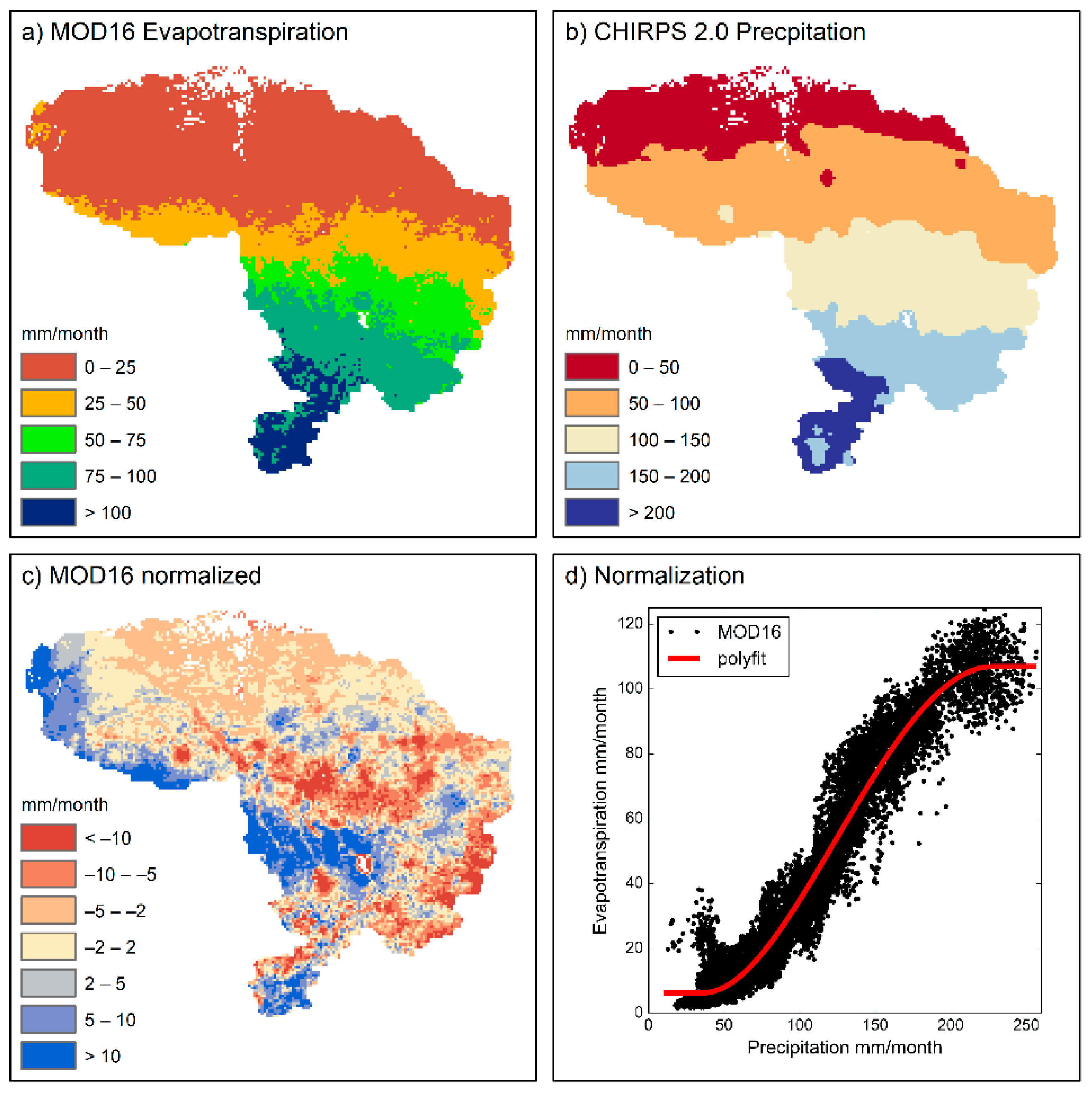
For the trend function we fitted a 4th degree polynomial function with truncated tails to model ET based on precipitation as the only input. A polynomial function was chosen due to its capability of modelling a broad range of non-linear relationships. The coefficient of determination (R²) between the fitted polynomial trend function and the data is 0.96. The method is illustrated in Figure 3, where the North-South precipitation gradient that causes the ET trend is apparent. The upper tail of the ET and precipitation relationship is flat, suggesting energy limited conditions. The high ET values found for low precipitation values are located in the western coastal region of the Senegal River basin and are likely caused by intensive irrigation activities in the delta. The effect of climate normalization becomes apparent in Figure 3, the original ET pattern is a direct imprint of the precipitation pattern, whereas the normalized pattern conveys more complexity of the hydrological processes taking place in the basin. The normalized pattern is normally distributed with a mean of zero and captures the deviation of the original ET pattern to the fitted trend model. Positive values are partly correlated with a higher clay content, due to the better water-holding capacity of clayey soils and LAI is found to be higher for positive values of normalized ET (not shown).

For the spatial pattern evaluation of the simulated normalized ET we employed the same trend function as applied to normalize observed ET. To accommodate any potential bias between the observed ET and the hydrological model, the ET bias of the model is added to the trend function before the normalization is applied.

2.6. Calibration Experiments

Two calibration experiments were performed with the model-independent Ostrich optimization software [45] using the ParaPADDS search algorithm. ParaPADDS is a parallelized multi-objective Dynamically Dimension Search (DDS) [46] algorithm that identifies a Pareto front of non-dominated optimal solutions, which is particularly useful for multi-objective calibrations. The ParaPADDS algorithm was run with the user settings of 2000 iterations, with 3 parallel runs, a 0.2 perturbation value and the ExactHyperVolumeContribution as the selection metric. In this study, two objective functions (OFs) were used for the model calibration. Ostrich minimizes any given OF and since KGE and SPAEF have an optimal value of 1 we calculated the squared residuals for each of the two OFs.

$$S{R}_{ET}={\left(1-SPAEF\right)}^2,$$

(4)

where $S{R}_{ET}$ represents the squared residuals for the long-term average rainy season ET model performance applying SPAEF as OF. For Q, KGE was calculated at four stations and here we used the sum of squared residuals.

$$SS{R}_Q={\sum }_i^4{\left(1-KG{E}_i\right)}^2,$$

(5)

where $SS{R}_Q$ represents the sum of squared residuals for the Q performance at four discharge stations using KGE as OF.

We have designed two calibration experiments to investigate the potential benefits of climate normalization. Both calibrations used $SS{R}_Q$ as objective function. An additional objective function, Cal1, used $S{R}_{ET}$ based on the original rainy season ET climatology, whereas Cal2 used $S{R}_{ET}$ based on the normalized rainy season ET climatology. In the SPAEF formulation, $\alpha$ is the coefficient of determination fraction. To avoid division by zero for the coefficient of determination, SPAEF for the normalized patterns was based on the fraction of standard deviations for the $\alpha$ component, as opposed to the fraction of coefficients of determination Equation (2). This is justifiable, because normalization will result in spatial patterns with a mean of zero.

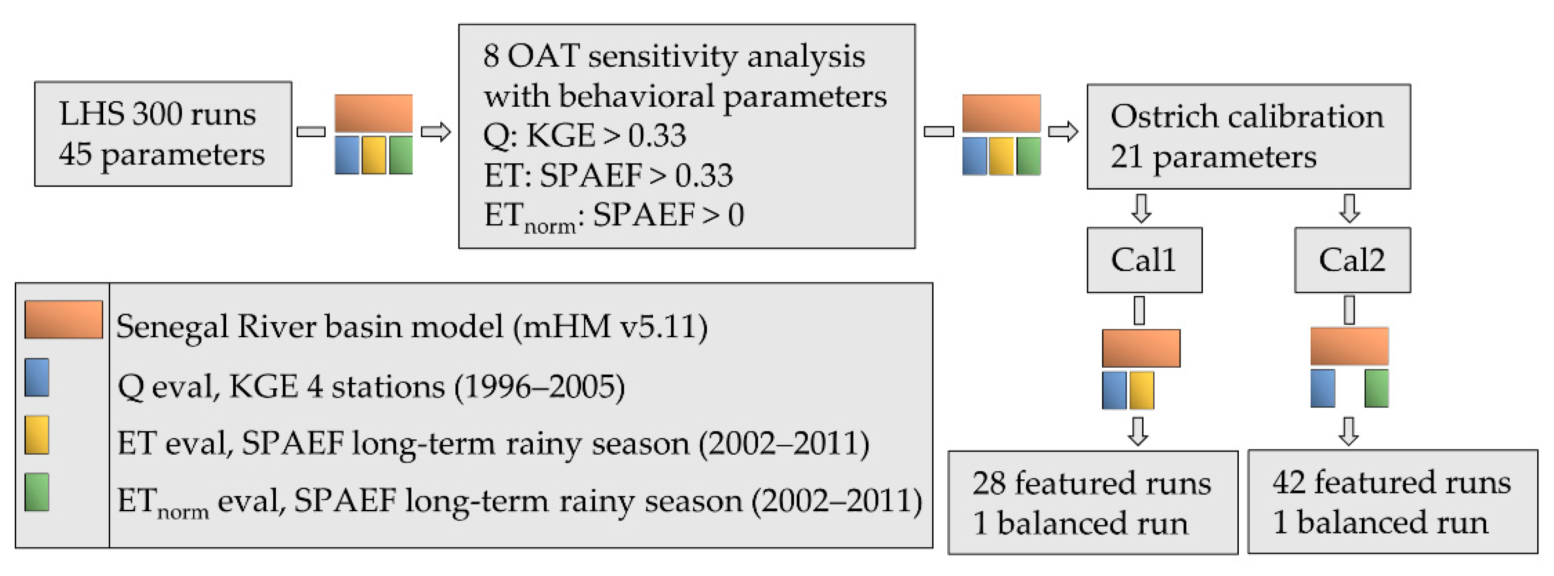
Prior to calibration, we conducted a comprehensive sensitivity analysis to select the calibration parameters. The sensitivity analysis was based on a one-at-a-time (OAT) perturbation of model parameters and the change in OF was recorded to assess sensitivity. In order to overcome the limitation of the OAT perturbation, which only captures local sensitivity, we designed an ensemble approach taking multiple initial parameter sets into consideration [47]. We selected 8 behavioral initial parameter sets for the OAT sensitivity analysis, i.e., KGE for all four Q stations and SPAEF for the original ET pattern greater than 0.33 as well as a positive SPAEF for the normalized ET pattern. The behavioral parameter sets were obtained from a Latin Hypercube Sampling (LHS) of 300 initial parameter sets. The flow chart in Figure 4 provides an overview of the modelling steps and calibration experiments.

3. Results

3.1. Sensitivity Analysis

The results of the sensitivity analysis are based on the eight behavioral parameter sets that were employed in a local OAT sensitivity analysis. The sensitivity for a given parameter perturbation was recorded for the three defined OFs, namely KGE at four discharge stations, and SPAEF for the original and the normalized rainy season ET pattern. Each set of sensitivities was normalized per OF by the maximum to range between 0 and 1. In total, 21 out of the 45 parameters were selected for subsequent model calibration and the sensitivities for those parameters are shown in Figure 5. The 21 parameters are stated in

Table 1. The 21 mHM parameters selected for calibration and their calibrated values for the featured runs of Cal1 and Cal2. Pedo transfer function is abbreviated with ptf.

Parameter Name	Description	Cal1	Cal2
canintfact	canopy interception factor	0.110	0.120
ptflowconst	ptf saturated water content: constant	0.876	0.700
ptflowclay	ptf saturated water content: coefficient clay content	0.002	0.001
ptflowdb	ptf saturated water content: coefficient bulk density	0.255	0.159
ptfhigconst	ptf saturated water content: constant	0.749	0.795
ptfhigdb	ptf saturated water content: coefficient bulk density	0.100	0.100
ptfksconst	ptf hydraulic conductivity: constant	0.574	0.600
ptfkssand	ptf hydraulic conductivity: coefficient sand content	0.012	0.013
ptfksclay	ptf hydraulic conductivity: coefficient clay content	0.015	0.015
rotfrcoffor	root fraction coefficient forest	0.990	0.990
rotfrcofsa	root fraction coefficient sand	0.001	0.001
rotfrcofcl	root fraction coefficient clay	0.995	0.993
fcmin	field capacity scaling: minimum	0.108	0.044
fcdelta	field capacity scaling: range	0.300	0.496
jarvis	jarvis soil moisture threshold	0.996	0.994
infshapef	infiltration shape factor	1.610	1.410
pet_af	PET scaling: minimum forest	0.504	0.500
pet_ap	PET scaling: minimum permeable	0.552	0.516
pet_b	PET scaling: range	2.190	2.880
pet_c	PET scaling: shape	0.154	0.145

.

With respect to the different OFs, different parameters were identified as sensitive. Discharge is controlled by the root fraction parameter for forest (rotfrcoffore) and the soil type dependent root fraction parameter (rotfrcofcl). These parameters control the vertical distribution of roots and thereby they affect the water balance, i.e., the partitioning into soil water available for transpiration and runoff generation. Furthermore, two pedo transfer function parameters that control the saturated water content (ptflowconst and ptflowdb) are identified as being sensitive for the simulation of discharge. The spatial pattern of ET is sensitive to the root fraction parameters as well as for the PET scaling function that estimates a spatially distributed crop coefficient. The most sensitive parameters are the maximum and minimum of the crop coefficient (pet_b and pet_a, respectively), as well as the shape of the exponential function (pet_c). The sensitivities for the normalized ET pattern diverge with respect to the original ET pattern. Here, the pedo transfer parameters, as well as the PET scaling function, are more sensitive and the forest root fraction (rotfrcoffore) is less sensitive. The variability of the ensemble is apparent for some, but not for all parameters. For example, the soil type dependent root fraction parameter (rotfrcofcl) is the most sensitive parameter for all eight initial parameter sets for the normalized ET patterns, whereas the sensitive for forest root fraction (rotfrcoffore) parameter varies between the eight initial parameter sets for SPAEF calculated for the original ET patterns.

3.2. Pareto Front

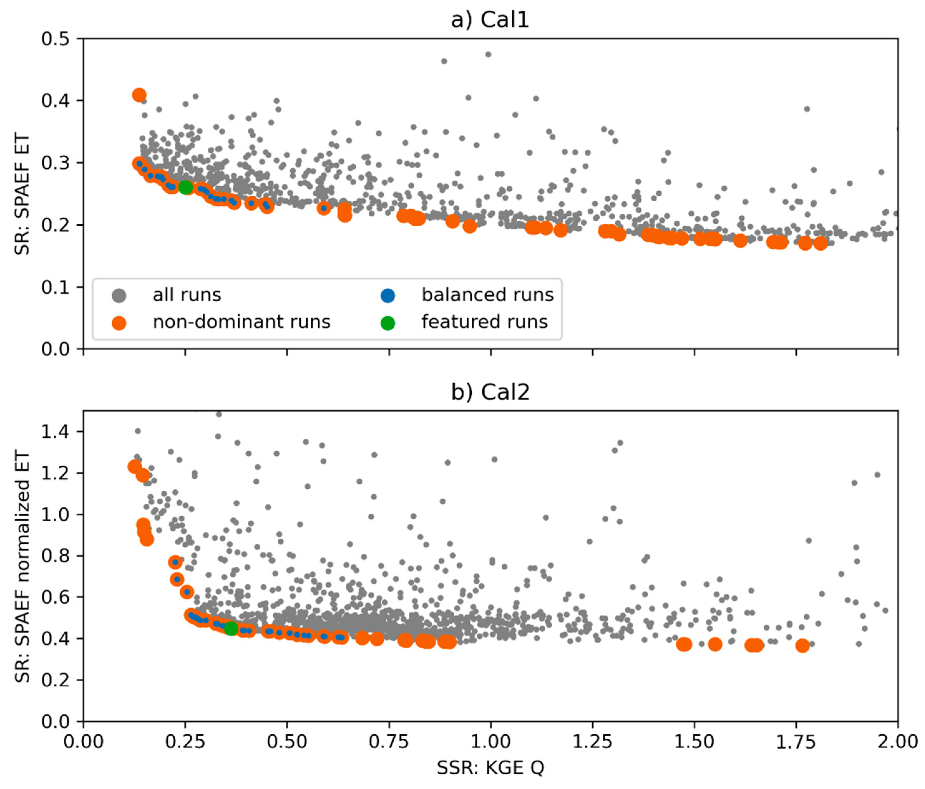
The results of the two calibration experiments are presented in 6. Each calibration comprised 2000 model runs and the non-dominated runs, which mark the pareto front, were identified by Ostrich. The characteristic of a non-dominated run is that one OF cannot be improved without compromising the other. Ostrich does not provide the user with an optimal run, instead it is up to the user to study the tradeoff between the applied OFs to select a parameter set or an ensemble for subsequent model application. The distribution of runs along the pareto front contains an element of randomness as it is a result of the ParaPADDS search algorithm. Both calibrations depict a clear pareto front describing the tradeoff between the temporal discharge performance and the spatial ET performance. The SPAEF residuals for the normalized ET patterns are larger than for the original ET patterns which indicates that the simulated patterns after normalization are more dissimilar to the normalized target pattern than the original ET patterns. Opposed to this, the discharge performance is comparable between the two calibrations.

In order to investigate the two calibration experiments in more detail, we have selected a subset of the non-dominated runs. This subset contained balanced runs which are located around the optimum, disregarding the tails of the pareto front which focus solely on a single OF. This selection results in what is referred to as the balanced sets in Figure 6a,b. For the selection, the tail of high KGE residuals was truncated by the median KGE plus one standard deviation and the for the SPAEF residuals, values that exceed median SPAEF plus three standard deviations were excluded. For each calibration, a single run was selected as a featured run in order to visualize simulation results and the parameter sets of the featured runs of Cal1 and Cal2 are stated in Table 1.

For Cal1, the amount of selected balanced runs was 28, and for Cal2, 42 runs were selected as balanced runs. The deviation is simply a result of how ParaPADDS samples the parameter space and should not be understood as a degree of robustness of the two calibrations.

Table 2. Summary of the calibration results taking only the balanced runs into consideration. The number of runs that are contained in the ensemble varies between the two calibrations and median and standard deviation (std) of the ensembles are presented. The three components of the SPAEF are stated: Correlation (r), variability (α) and distribution (β).

		Q	ET				Normalized ET
		KGE	SPAEF	r	α	β	SPAEF	r	α	β
Cal1 n = 28	median	0.73	0.49	0.97	0.56	0.74	0.23	0.28	1.07	0.75
	std	0.05	0.02	0.00	0.01	0.01	0.08	0.05	0.12	0.04
Cal2 n = 42	median	0.70	0.52	0.97	0.58	0.75	0.33	0.37	0.99	0.78
	std	0.05	0.02	0.00	0.01	0.01	0.05	0.04	0.07	0.02

provides an overview of the median and standard deviation of the applied OFs computed for the balanced runs of Cal1 and Cal2. The discharge performance is comparable with a slight advantage of Cal1. The spatial pattern performance of ET, expressed as SPAEF, is also comparable between the calibrations even though Cal2 is not explicitly calibrated against the original ET patterns. Differences between the calibrations become apparent for the normalized ET performance. Here, Cal2, which is calibrated against the normalized patterns, stands out with an improvement in SPAEF by 0.1 with respect to Cal1. The three SPAEF components are also given in Table 2. For the original patterns, correlation is the dominating component which is close to optimal in both calibrations. Here, the variability component was simulated poorest by both calibrations. For the normalized ET evaluation, the scores of the individual SPAEF components varies more distinctly. In this case, the variability component was simulated best by both calibrations, whereas the correlation has the lowest scores and also the most apparent difference between Cal1 and Cal2.

3.3. Evapotranspiration Evaluation

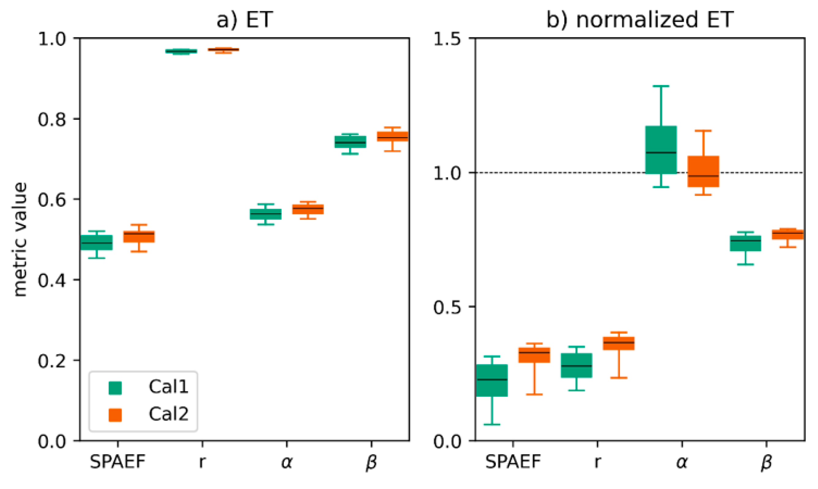
In order to further evaluate the simulated pattern of ET, Figure 7 elucidates the statistics provided in Table 2 in more detail. The balanced runs of Cal1 and Cal2 are cross-evaluated, i.e., the balanced runs obtained from Cal2 are also evaluated against the original ET patterns using SPAEF. Both calibrations show similar performance for the original ET pattern performance, in spite of the fact that Cal2 is only calibrated against the normalized pattern. The correlation component is close to one with a minimal variability. Cal1 and Cal2 show similar performance based on all three SPAEF components for the evaluation of the original ET pattern. For the normalized ET evaluation, Cal2 finds more accurate solutions (i.e., closer to 1) than Cal1. This results in an overall increase in SPAEF. Opposed to the original ET pattern evaluation, the normalized evaluation is less dominated by the correlation term and the inter-quantile range for each metric of the balanced runs is also larger.

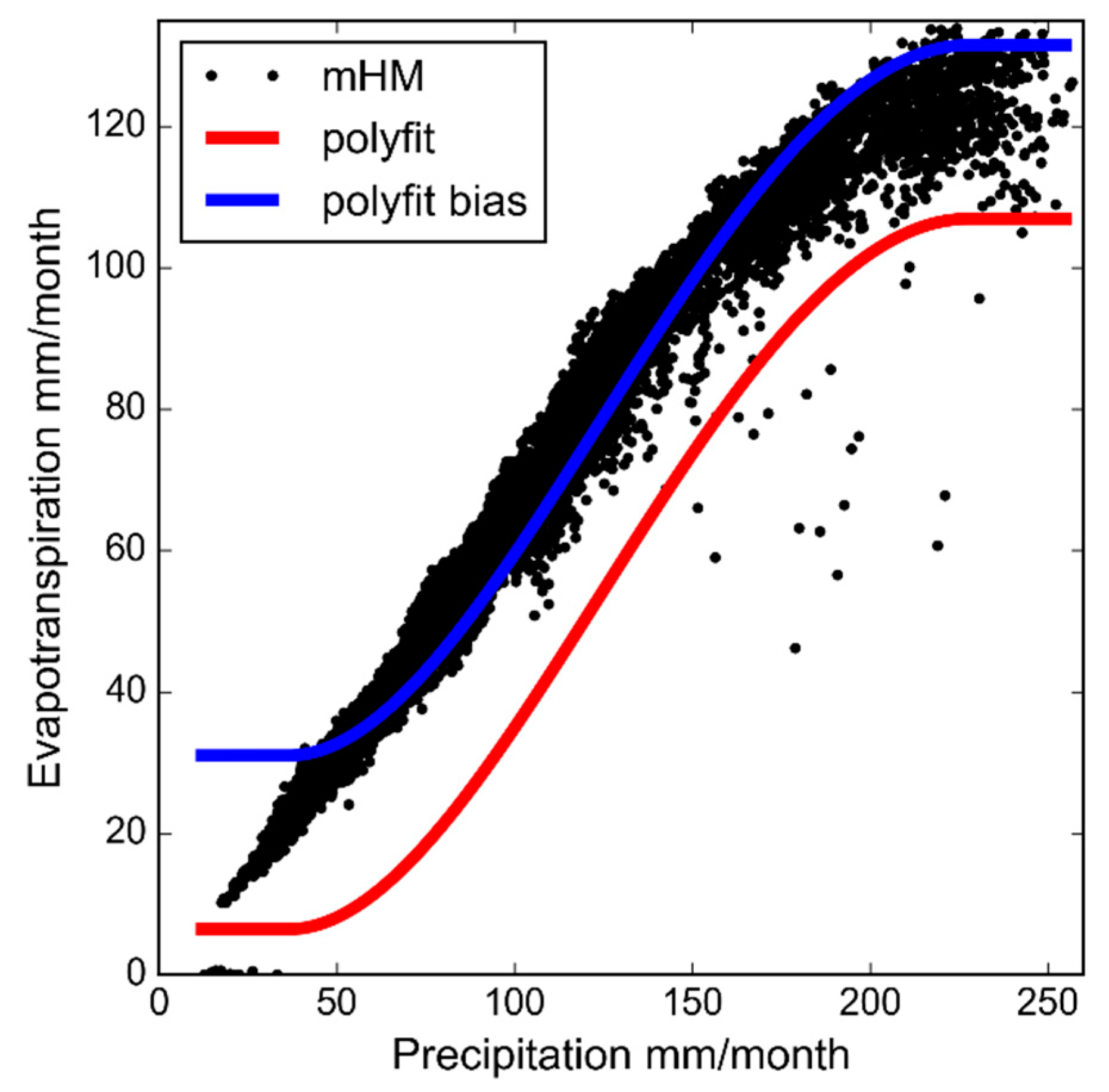
The climate normalization of the simulated ET data is visualized in Figure 8. The proposed normalization framework accepts any potential bias inherent to the simulation. Thus, the polynomial model fitted to the observed ET data is shifted, taking into account the simulation bias. In our case, the model has a positive bias of around 30 mm mth⁻¹. The simulation captures the flattening of the relationship between precipitation and ET once energy-limited conditions are present. The observed flattening at the dry end, which is evident in the MOD16 data, is not captured accordingly by the model and instead simulated ET continuous to decrease with decreasing precipitation. Furthermore, the high ET rates found at the dry end of the plot in Figure 3, which can be attributed to irrigation, are not captured since irrigation is not among the described processes in mHM. Both Table 2 and Figure 7 underline that the variability component is captured quite accurately by Cal1 and Cal2 for the normalized pattern. Basically, this component describes the deviation from the trend line and by taking the model bias into account, the variability can be adequately matched by the model despite any potential bias.

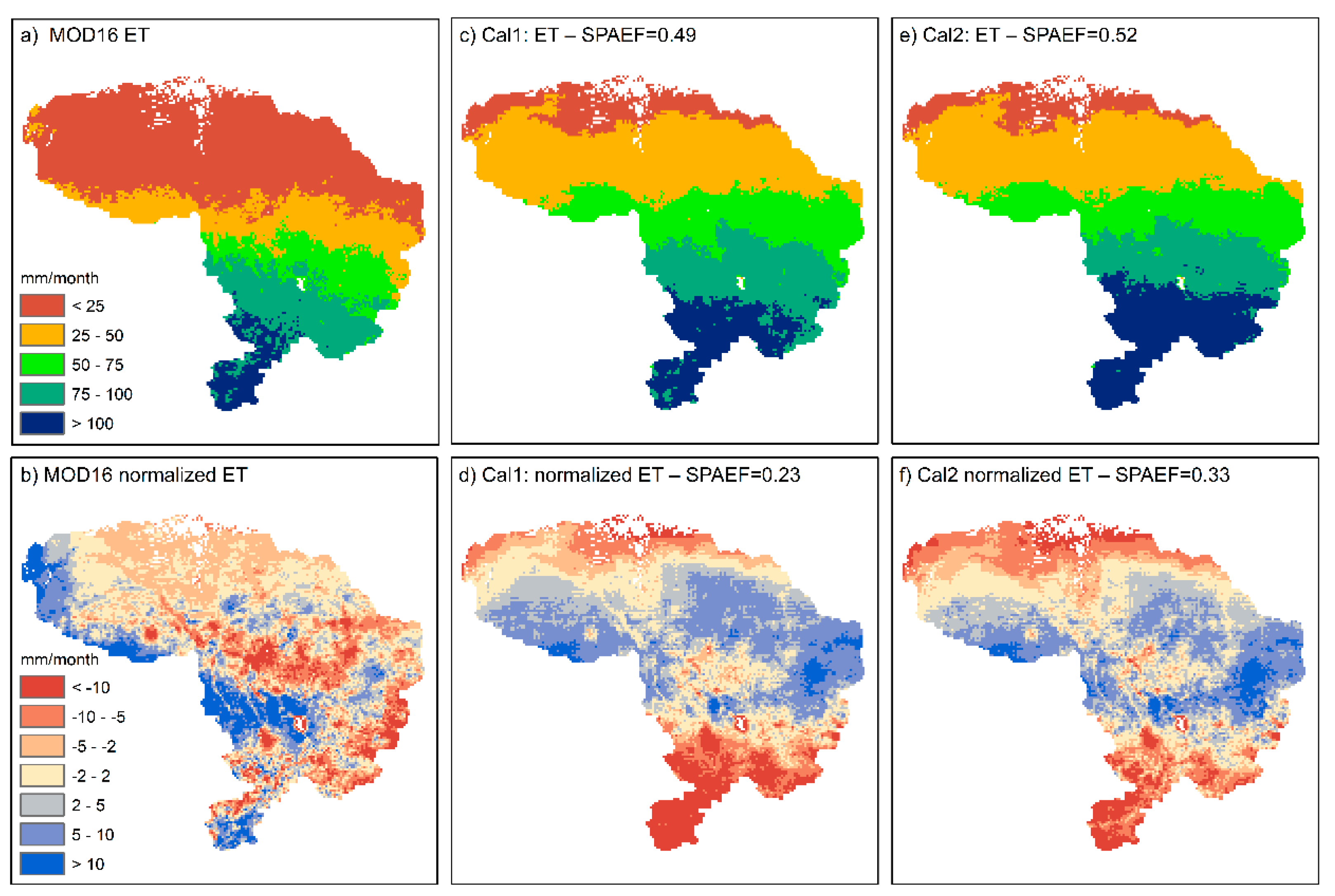
The simulated spatial patterns of ET obtained from the balanced runs from Cal1 and Cal2 with respect to the observed rainy season pattern (MOD16) are shown in Figure 9. Despite the notable bias, the original pattern of Cal1 and Cal2 both reflect the north-south trend accordingly. Since the calibration utilizes a bias insensitive objective function, i.e., SPAEF, the simulation bias in ET is acceptable. The SPAEF-based evaluation attests a slightly better pattern performance to Cal2 than Cal1. The normalized rainy season ET pattern contains more complexity, and it becomes obviously more challenging to achieve a satisfying pattern performance. Based on the SPAEF evaluation Cal2 is more accurate than Cal1 in capturing the normalized ET pattern. Visually, there lacks resemblance between the observed normalized pattern for both calibrations. Some similarity is notable, e.g., negative values in the northern part, central part and eastern part of the Senegal River basin. However, many details of the spatial pattern are not captured by the model.

3.4. Discharge Evaluation

Figure 10 presents the discharge evaluation at the four gauging stations using continuous daily observations over a 10-year period. The simulated Q was obtained from the featured runs (Figure 6) and in terms of KGE, Cal1 tends to perform better or at least as good as Cal2 at all four stations. The Gourbassa station obtained the highest KGE scores for both calibration experiments, whereas the Dakka stations showed the poorest results. For the latter, the model failed to reproduce the delayed flows towards the end of the rainy season. Overall, interannual variability is captured by the model since magnitude of the high flows follows the observations.

4. Discussion

4.1. Normalization Method

The proposed grid-based normalization method is based on a fitted polynomial trend model. The deviation of ET with respect to the trend model provides information on to what extent ET, at a given location with a certain precipitation input, is higher or lower than an expected ET flux derived from the trend model. In principle, this information is expected to relate to physical basin properties, i.e., better water holding capacity in clayey soils resulting in positive normalized values and sparse vegetation resulting in negative normalized values as a consequence of reduced transpiration and increased surface runoff or recharge. This process heterogeneity can be related to model parameters that are optimizable through calibration. An alternative precipitation normalization strategy is to simply calculate the evaporation index by dividing ET with precipitation [21]. This index provides information on the degree of water limitation and precipitation partitioning of a grid cell, but does not reflect any potential non-linearity contained in the relationship between ET and precipitation. Further, a potential bias in the simulation may pose a challenge in the calculation and comparison between an observed and a simulated evaporation index.

In the proposed normalization, the simulation bias is taken into account by shifting the trend model up or down based on the sign and magnitude of the bias. This works effectively (Figure 8) and falls in line with the general notion of bias-insensitivity for spatial pattern-oriented model evaluations [10,13].

An advantage of the proposed normalization method is that, in principle, the method is applicable for different variables causing a gradient associated to an observed spatial pattern. This could for example be PET or air temperature when evaluating the spatial pattern performance of a large-scale basin with a distinct climate gradient or a smaller basin with a distinct topography gradient. The topography and air temperature normalization would especially be relevant for LST evaluations whereas PET normalization would be useful for ET evaluations. We consider normalization of remotely sensed SM as an alternative prospect since gradients in SM, just like ET, are often controlled by precipitation or other climate variables [12]. In basins with more complex gradients, multi-variate trend models could also be an option for the normalization.

The Senegal River basin, with its distinct north-south climate gradient, was a perfect testbed for developing the proposed normalization technique. Future research should investigate basins with gradients driven by alternative processes.

4.2. Calibration Strategy

The Pareto fronts obtained by the ParaPADDS algorithm showed well-defined tradeoffs between Q and ET performance for both calibration experiments. In theory, all Pareto optimal solutions (non-dominated) can be considered candidates for the “best fit” parameter set. In this study, we tried to avoid identifying a single run as the optimal solution, although “featured runs” were selected for visualization purposes. Instead, we focused on selecting a subset of the full Pareto front containing balanced solutions. This subset was treated as an ensemble and the statistics of the OFs were subsequently analyzed.

The multi-component SPAEF metric allows the spatial pattern performance of a model to be interpreted in more detail. For example, we found that Cal1 was largely dominated by correlation, because the allocation of high and low ET was constrained by the precipitation input and thus, the effect of model parameters was largely overshadowed. The correlation component of SPAEF in Cal2 was largely reduced since the normalized pattern was not controlled by the precipitation forcing and instead the effect of model parameters is expected to be more prominent. The Q performance can be regarded as comparable between the two calibration experiments, even though Cal1 is slightly in favor with respect to the balanced runs (Table 2). It was not anticipated that the balanced runs of Cal2 resulted in a better spatial pattern performance for the original ET pattern than Cal1. However, the slightly reduced Q performance of the balanced runs of Cal2 may explain this. In general terms, this may also relate to the way the balanced runs were selected and how the calibration evolved.

Any potential bias inherent to the selected ET reference dataset is addressed in multiple ways. First, the three components of the SPAEF metric are bias insensitive which puts sole focus on the spatial pattern evaluation, because our credibility of the magnitude of the pattern contained in remotely sensed ET datasets is low, but we regard the spatial pattern information as more trustworthy [15]. Second, the SPAEF is calculated based on simulated and observed log-term average climatologies of ET, which are in principle less uncertain, because uncertainties at monthly or sub-monthly timescales due to uncertain climate variability are alleviated. Third, the proposed climate normalization strategy takes the simulation bias into account by adding the bias to the trend model.

Even though the improvement with respect to the normalized pattern performance of Cal2 (SPAEF = 0.33) in comparison to Cal1 (SPAEF = 0.23) is clear, i.e., a 30% decrease going from Cal2 to Cal1, the visual assessment of the featured runs in Figure 9 is difficult to interpret. The normalized pattern from Cal2 possesses more variability, especially in the southern part of the Senegal River basin, which resulted in an improved SPAEF score with respect to Cal1. The incapacity of the model to further improve the normalized ET pattern performance through calibration may related to the quality of the input data, i.e., spatially distributed soil data or vegetation data, or a limited flexibility of the applied parametrization scheme. Moreover, the reference ET dataset, which was derived from MODIS for the purpose of this study, may be inadequate and investigating alternative sources of ET could be an additional way to proceed.

4.3. Limitations

A limitation of the normalization strategy is that manual fitting of the polynomial trend model is required. This may pose problems when calibrating multiple basins, utilizing alternative ET sources, or just evaluating a different time period, because an individual trend model has to be fitted for each normalization. A more general limitation of the study is that only a single combination of precipitation and ET sources have been applied in the calibration. It has been highlighted that the quality of ET products varies greatly across Africa [42] and given the low density of ground-truth flux towers it remains a challenge to identify a single most useful product. The same holds for precipitation [48]. Ideally, the related uncertainties are explored in detail by an ensemble approach where combinations of alternative precipitation and evapotranspiration data sources are utilized in a comprehensive calibration experiment [31,32]. Additionally, a multi-model ensemble can be implemented to explore uncertainties associated to model structure [49,50] or even combining the multi-model approach with multi forcing datasets [51]. However, since the focus of this study was to initially test the climate normalization strategy, such a comprehensive calibration experiment was beyond the scope. The robustness of the calibration experiments and the effectiveness of the proposed normalization strategy should be investigated in more detail in future studies.

Along these lines, the usefulness of a normalized spatial pattern of a remotely sensed hydrological variable depends on the quality of the data. In this study, the quality of the precipitation data is essential, and precipitation uncertainties may introduce errors in the normalized pattern which may hamper the calibration. Nevertheless, the precipitation utilized in the normalization is the same as being used as forcing in the hydrological model. Therefore, artefacts in the normalization caused by erroneous precipitation data may be compensated by the hydrological model which uses the same data as input.

With respect to the selected satellite-based ET product, MOD16, it must be highlighted that by choosing the MODIS ET product, we do not imply that it is the most suitable for the Senegal River basin. There are numerous alternative ET datasets readily available and as shown, for Africa, their accuracy varies greatly [42]. It was found that, based on the water balance approach (precipitation minus runoff) annual ET for the Senegal River basin is below 500 m yr⁻¹ and the bias of nine studied ET products ranges from −125 mm to +200 mm. However, since we apply a bias insensitive spatial pattern objective function (SPAEF) the magnitude of the satellite-based ET product is less crucial and the accuracy of the spatial pattern, which is targeted by the chosen objective function, is difficult to assess.

5. Conclusions

Recent advances of spatial pattern-oriented model evaluations utilizing satellite remote sensing data have motivated us to investigate the Senegal River basin, a basin dominated by a strong climate gradient, in more detail. We conducted two calibration experiments using remotely sensed ET patterns in an original and precipitation normalized form as objective functions to test our hypothesis that climate gradients overshadow the sensitivity of model parameters on the simulated spatial patterns. We can draw the following main conclusions from our work:

(1)

The multi-objective calibration of the Senegal River basin resulted in a well-defined Pareto front that highlighted tradeoffs between the temporal Q performance at four stations and the spatial pattern performance for long-term average rainy-season ET.

(2)

Climate normalizing of ET was successfully implemented using a polynomial trend model linking the distinct north-south gradient in precipitation to the spatial pattern of ET. The normalized spatial pattern conveys more complexity, i.e., hydrological processes related to soil and vegetation variability, than the original spatial pattern.

(3)

The sensitivity of model parameters varied between the original ET pattern and the normalized ET pattern which supported the conclusion that the normalized pattern contained alternative information related to different processes.

(4)

Calibrating against climate normalized patterns did not compromise the performance of the original patterns and a very comparable performance was obtained between the two calibration experiments for the original ET pattern. However, the spatial pattern performance for the normalized pattern increased from SPAEF = 0.23 in Cal1 to SPAEF = 0.33 in Cal2.

References

1. Demirel, M.C.; Mai, J.; Mendiguren, G.; Koch, J.; Samaniego, L.; Stisen, S. Combining satellite data and appropriate objective functions for improved spatial pattern performance of a distributed hydrologic model. Hydrol. Earth Syst. Sci. 2018, 22, 1299–1315. [Google Scholar] [CrossRef] [Green Version]
2. Mendiguren, G.; Koch, J.; Stisen, S. Spatial pattern evaluation of a calibrated national hydrological model—A remote-sensing-based diagnostic approach. Hydrol. Earth Syst. Sci. 2017, 21, 5987–6005. [Google Scholar] [CrossRef] [Green Version]
3. Soltani, M.; Bjerre, E.; Koch, J.; Stisen, S. Integrating remote sensing data in optimization of a national water resources model to improve the spatial pattern performance of evapotranspiration. J. Hydrol. 2021, 603, 127026. [Google Scholar] [CrossRef]
4. Hunink, J.E.; Eekhout, J.P.C.; de Vente, J.; Contreras, S.; Droogers, P.; Baille, A. Hydrological Modelling using Satellite-based Crop Coefficients: A Comparison of Methods at the Basin Scale. Remote Sens. 2017, 9, 174. [Google Scholar] [CrossRef] [Green Version]
5. Samaniego, L.; Kumar, R.; Thober, S.; Rakovec, O.; Zink, M.; Wanders, N.; Eisner, S.; Müller Schmied, H.; Sutanudjaja, E.; Warrach-Sagi, K.; et al. Toward seamless hydrologic predictions across spatial scales. Hydrol. Earth Syst. Sci. 2017, 21, 4323–4346. [Google Scholar] [CrossRef] [Green Version]
6. Mizukami, N.; Clark, M.P.; Newman, A.J.; Wood, A.W.; Gutmann, E.D.; Nijssen, B.; Rakovec, O.; Samaniego, L. Towards seamless large-domain parameter estimation for hydrologic models. Water Resour. Res. 2017, 53, 8020–8040. [Google Scholar] [CrossRef]
7. Conradt, T.; Wechsung, F.; Bronstert, A. Three perceptions of the evapotranspiration landscape: Comparing spatial patterns from a distributed hydrological model, remotely sensed surface temperatures, and sub-basin water balances. Hydrol. Earth Syst. Sci. 2013, 17, 2947–2966. [Google Scholar] [CrossRef] [Green Version]
8. Koch, J.; Jensen, K.H.; Stisen, S. Toward a true spatial model evaluation in distributed hydrological modeling: Kappa statistics, Fuzzy theory, and EOF-analysis benchmarked by the human perception and evaluated against a modeling case study. Water Resour. Res. 2015, 51, 1225–1246. [Google Scholar] [CrossRef]
9. Stisen, S.; Koch, J.; Sonnenborg, T.O.; Refsgaard, J.C.; Bircher, S.; Ringgaard, R.; Jensen, K.H. Moving beyond run-off calibration —Multivariable optimization of a surface-subsurface-atmosphere model. Hydrol. Process. 2018, 32, 2654–2668. [Google Scholar] [CrossRef]
10. Koch, J.; Demirel, M.C.; Stisen, S. The SPAtial EFficiency metric (SPAEF): Multiple-component evaluation of spatial patterns for optimization of hydrological models. Geosci. Model Dev. 2018, 11, 1873–1886. [Google Scholar] [CrossRef] [Green Version]
11. Zink, M.; Mai, J.; Cuntz, M.; Samaniego, L. Conditioning a Hydrologic Model Using Patterns of Remotely Sensed Land Surface Temperature. Water Resour. Res. 2018, 54, 2976–2998. [Google Scholar] [CrossRef]
12. Dembélé, M.; Hrachowitz, M.; Savenije, H.H.G.; Mariéthoz, G.; Schaefli, B. Improving the Predictive Skill of a Distributed Hydrological Model by Calibration on Spatial Patterns With Multiple Satellite Data Sets. Water Resour. Res. 2020, 56, e2019WR026085. [Google Scholar] [CrossRef]
13. Koch, J.; Siemann, A.; Stisen, S.; Sheffield, J. Spatial validation of large scale land surface models against monthly land surface temperature patterns using innovative performance metrics. J. Geophys. Res. Atmos. 2016, 121, 5430–5452. [Google Scholar] [CrossRef]
14. Ko, A.; Mascaro, G.; Vivoni, E.R. Strategies to Improve and Evaluate Physics-Based Hyperresolution Hydrologic Simulations at Regional Basin Scales. Water Resour. Res. 2019, 55, 1129–1152. [Google Scholar] [CrossRef]
15. Stisen, S.; Soltani, M.; Mendiguren, G.; Langkilde, H.; Garcia, M.; Koch, J. Spatial patterns in actual evapotranspiration climatologies for europe. Remote Sens. 2021, 13, 2410. [Google Scholar] [CrossRef]
16. Rakovec, O.; Mizukami, N.; Kumar, R.; Newman, A.J.; Thober, S.; Wood, A.W.; Clark, M.P.; Samaniego, L. Diagnostic Evaluation of Large-Domain Hydrologic Models Calibrated Across the Contiguous United States. J. Geophys. Res. Atmos. 2019, 124, 13991–14007. [Google Scholar] [CrossRef] [Green Version]
17. Koster, R.D.; Mahanama, S.P.P. Land surface controls on hydroclimatic means and variability. J. Hydrometeorol. 2012, 13, 1604–1620. [Google Scholar] [CrossRef]
18. Guzinski, R.; Nieto, H.; Stisen, S.; Fensholt, R. Inter-comparison of energy balance and hydrological models for land surface energy flux estimation over a whole river catchment. Hydrol. Earth Syst. Sci. 2015, 19, 2017–2036. [Google Scholar] [CrossRef] [Green Version]
19. Budyko, M.I. Climate and Life; Academic Press Inc.: New York, NY, USA, 1974; 508p. [Google Scholar]
20. Greve, P.; Burek, P.; Wada, Y. Using the Budyko Framework for Calibrating a Global Hydrological Model. Water Resour. Res. 2020, 56, e2019WR026280. [Google Scholar] [CrossRef]
21. Kushwaha, A.P.; Tiwari, A.D.; Dangar, S.; Shah, H.; Mahto, S.S.; Mishra, V. Multimodel assessment of water budget in Indian sub-continental river basins. J. Hydrol. 2021, 603, 126977. [Google Scholar] [CrossRef]
22. Gharari, S.; Shafiei, M.; Hrachowitz, M.; Kumar, R.; Fenicia, F.; Gupta, H.V.; Savenije, H.H.G. A constraint-based search algorithm for parameter identification of environmental models. Hydrol. Earth Syst. Sci. 2014, 18, 4861–4870. [Google Scholar] [CrossRef] [Green Version]
23. Samaniego, L.; Kumar, R.; Attinger, S. Multiscale parameter regionalization of a grid-based hydrologic model at the mesoscale. Water Resour. Res. 2010, 46, W05523. [Google Scholar] [CrossRef] [Green Version]
24. Kumar, R.; Samaniego, L.; Attinger, S. Implications of distributed hydrologic model parameterization on water fluxes at multiple scales and locations. Water Resour. Res. 2013, 49, 360–379. [Google Scholar] [CrossRef]
25. Stisen, S.; Jensen, K.H.; Sandholt, I.; Grimes, D.I.F. A remote sensing driven distributed hydrological model of the Senegal River basin. J. Hydrol. 2008, 354, 131–148. [Google Scholar] [CrossRef]
26. Bodian, A.; Diop, L.; Panthou, G.; Dacosta, H.; Deme, A.; Dezetter, A.; Ndiaye, P.M.; Diouf, I.; Visch, T. Recent trend in hydroclimatic conditions in the Senegal River basin. Water 2020, 12, 436. [Google Scholar] [CrossRef] [Green Version]
27. Samaniego, L.; Brenner, J.; Craven, J.; Cuntz, M.; Dalmasso, G.; Demirel, C.M.; Jing, M.; Kaluza, M.; Kumar, R.; Langenberg, B.; et al. Mesoscale Hydrologic Model-mHM. v5.11.1. 2021. Available online: https://www.ufz.de/index.php?en=40114 (accessed on 6 January 2022).
28. Thober, S.; Cuntz, M.; Kelbling, M.; Kumar, R.; Mai, J.; Samaniego, L. The multiscale routing model mRM v1.0: Simple river routing at resolutions from 1 to 50 km. Geosci. Model Dev. 2019, 12, 2501–2521. [Google Scholar] [CrossRef] [Green Version]
29. Kumar, R.; Livneh, B.; Samaniego, L. Toward computationally efficient large-scale hydrologic predictions with a multiscale regionalization scheme. Water Resour. Res. 2013, 49, 5700–5714. [Google Scholar] [CrossRef]
30. Poméon, T.; Diekkrüger, B.; Kumar, R. Computationally efficient multivariate calibration and validation of a grid-based hydrologic model in sparsely gauged West African river basins. Water 2018, 10, 1418. [Google Scholar] [CrossRef] [Green Version]
31. Dembélé, M.; Ceperley, N.; Zwart, S.J.; Salvadore, E.; Mariethoz, G.; Schaefli, B. Potential of satellite and reanalysis evaporation datasets for hydrological modelling under various model calibration strategies. Adv. Water Resour. 2020, 143, 103667. [Google Scholar] [CrossRef]
32. Dembele, M.; Schaefli, B.; Van De Giesen, N. Suitability of 17 gridded rainfall and temperature datasets for large-scale hydrological modelling in West Africa. Hydrol. Earth Syst. Sci. 2020, 24, 5379–5406. [Google Scholar] [CrossRef]
33. Hengl, T.; Heuvelink, G.B.M.; Kempen, B.; Leenaars, J.G.B.; Walsh, M.G.; Shepherd, K.D.; Sila, A.; MacMillan, R.A.; De Jesus, J.M.; Tamene, L.; et al. Mapping soil properties of Africa at 250 m resolution: Random forests significantly improve current predictions. PLoS ONE 2015, 10, e0125814. [Google Scholar] [CrossRef]
34. Friedl, M.; Gray, J.; Sulla-Menashe, D. MCD12Q2 MODIS/Terra+Aqua Land Cover Dynamics Yearly L3 Global 500m SIN Grid V006. Available online: https://lpdaac.usgs.gov/products/mcd12q2v006/ (accessed on 6 August 2021).
35. Myneni, R.B.; Knyazikhin, Y.; Park, T. MCD15A2H MODIS/Terra+Aqua Leaf Area Index/FPAR 8-Day L4 Global 500m SIN Grid V006. Available online: https://doi.org/10.5067/MODIS/MCD15A2H.006 (accessed on 6 August 2021).
36. Hersbach, H.; Bell, B.; Berrisford, P.; Hirahara, S.; Horányi, A.; Muñoz-Sabater, J.; Nicolas, J.; Peubey, C.; Radu, R.; Schepers, D.; et al. The ERA5 global reanalysis. Q. J. R. Meteorol. Soc. 2020, 147, 4186–4227. [Google Scholar] [CrossRef]
37. Hargreaves, G.H.; Samani, Z.A. Reference Crop Evapotranspiration from Temperature. Appl. Eng. Agric. 1985, 1, 96–99. [Google Scholar] [CrossRef]
38. Funk, C.; Peterson, P.; Landsfeld, M.; Pedreros, D.; Verdin, J.; Shukla, S.; Husak, G.; Rowland, J.; Harrison, L.; Hoell, A.; et al. The climate hazards infrared precipitation with stations—A new environmental record for monitoring extremes. Sci. Data 2015, 2, 150066. [Google Scholar] [CrossRef] [PubMed] [Green Version]
39. Funk, C.C.; Peterson, P.J.; Landsfeld, M.F.; Pedreros, D.H.; Verdin, J.P.; Rowland, J.D.; Romero, B.E.; Husak, G.J.; Michaelsen, J.C.; Verdin, A.P. A Quasi-Global Precipitation Time Series for Drought Monitoring; Data Series 832; US Geological Survey: Reston, VA, USA, 2014; pp. 1–12.
40. Running, S.; Mu, Q.; Zhao, M. MOD16A2 MODIS/Terra Net Evapotranspiration 8-Day L4 Global 500m SIN Grid V006. Available online: https://doi.org/10.5067/MODIS/MOD16A2.006 (accessed on 10 November 2021).
41. Hulsman, P.; Savenije, H.H.G.; Hrachowitz, M. Learning from satellite observations: Increased understanding of catchment processes through stepwise model improvement. Hydrol. Earth Syst. Sci. 2021, 25, 957–982. [Google Scholar] [CrossRef]
42. Weerasinghe, I.; Bastiaanssen, W.; Mul, M.; Jia, L.; Van Griensven, A. Can we trust remote sensing evapotranspiration products over Africa. Hydrol. Earth Syst. Sci. 2020, 24, 1565–1586. [Google Scholar] [CrossRef] [Green Version]
43. Gupta, H.V.; Kling, H.; Yilmaz, K.K.; Martinez, G.F. Decomposition of the mean squared error and NSE performance criteria: Implications for improving hydrological modelling. J. Hydrol. 2009, 377, 80–91. [Google Scholar] [CrossRef] [Green Version]
44. Knoben, W.J.M.; Freer, J.E.; Woods, R.A. Technical note: Inherent benchmark or not? Comparing Nash-Sutcliffe and Kling-Gupta efficiency scores. Hydrol. Earth Syst. Sci. 2019, 23, 4323–4331. [Google Scholar] [CrossRef] [Green Version]
45. Matott, L.S. OSTRICH: An Optimization Software Tool, Documentation and User’s Guide, version 17; University at Buffalo Center for Computational Research: Buffalo, NY, USA, 2017; p. 79. [Google Scholar]
46. Tolson, B.; Sharma, V.; Swayne, D.A. Parallel Implementations of the Dynamically Dimensioned Search (DDS) Algorithm. In Proceedings of the 7th International Symposium on Environmental Software Systems, Prague, Czech Republic, 22–25 May 2007. [Google Scholar]
47. Demirel, M.C.; Koch, J.; Mendiguren, G.; Stisen, S. Spatial pattern oriented multicriteria sensitivity analysis of a distributed hydrologic model. Water 2018, 10, 1188. [Google Scholar] [CrossRef] [Green Version]
48. Beck, H.E.; Vergopolan, N.; Pan, M.; Levizzani, V.; Van Dijk, A.I.J.M.; Weedon, G.P.; Brocca, L.; Pappenberger, F.; Huffman, G.J.; Wood, E.F. Global-scale evaluation of 22 precipitation datasets using gauge observations and hydrological modeling. Hydrol. Earth Syst. Sci. 2017, 21, 6201–6217. [Google Scholar] [CrossRef] [Green Version]
49. Dion, P.; Martel, J.L.; Arsenault, R. Hydrological ensemble forecasting using a multi-model framework. J. Hydrol. 2021, 600, 126537. [Google Scholar] [CrossRef]
50. Koch, J.; Cornelissen, T.; Fang, Z.; Bogena, H.; Diekkrüger, B.; Kollet, S.; Stisen, S. Inter-comparison of three distributed hydrological models with respect to seasonal variability of soil moisture patterns at a small forested catchment. J. Hydrol. 2016, 533, 234–249. [Google Scholar] [CrossRef]
51. Bhuiyan, M.A.E.; Nikolopoulos, E.I.; Anagnostou, E.N.; Polcher, J.; Albergel, C.; Dutra, E.; Fink, G.; Martínez-De La Torre, A.; Munier, S. Assessment of precipitation error propagation in multi-model global water resource reanalysis. Hydrol. Earth Syst. Sci. 2019, 23, 1973–1994. [Google Scholar] [CrossRef] [Green Version]
Figure 1. The Senegal River basin delineated as eight sub-catchments. The seven sub-catchments with available discharge records are stated by station names. The long-term average annual precipitation is based on CHIPRS 2.0 for the period of 1990–2019. The overview figure depicts the location of the Senegal River in Western Africa.
Remotesensing 14 00315 g001
Figure 2. Long-term climatologies of monthly evapotranspiration and precipitation for the Senegal River basin. Precipitation data are based on CHIPRS 2.0 and evapotranspiration data are retrieved from MODIS’ MOD16A2.006 product.
Remotesensing 14 00315 g002
Figure 3. Panel (a) depicts the long-term (2002–2011) average monthly rainy-season (June–November) evapotranspiration based on MOD16A2.006. Panel (b) shows the long-term average monthly rainy-season (June–November) precipitation based on CHIPRS 2.0. Panel (c) presents the precipitation normalized rainy-season evapotranspiration. The fitted polynomial model applied for the normalization is shown in panel (d).
Remotesensing 14 00315 g003
Figure 4. Flow chart of the conducted modelling work and calibration experiments.
Remotesensing 14 00315 g004
Figure 5. Results of the sensitivity analysis. The normalized sensitivity is given for the 21 parameters that were selected for subsequent model calibration. Sensitivity with respect to three objective functions is shown for the median of an ensemble of 8 different behavioral parameter sets. The whiskers represent the upper and lower limits of the inter-quantile range.
Remotesensing 14 00315 g005
Figure 6. Calibration results for Cal1 (panel (a)) and Cal2 (panel (b)). Each multi-objective calibration features 2000 runs (gray) of which the non-dominated runs (orange) were identified. The balanced runs (blue) represent an ensemble that is located around the pareto optimum. A single featured run (green) for both calibrations was selected to present simulation results.
Remotesensing 14 00315 g006
Figure 7. The spatial pattern evaluation of the balanced runs of Cal1 and Cal2 against the rainy-season ET climatology (panel (a)) and the precipitation normalized climatology (panel (b)). Metric values for SPAEF and its three components are presented. The boxplots show the median (black line), inter-quantile range (box) and 1st and 99th percentiles (whiskers).
Remotesensing 14 00315 g007
Figure 8. Example of simulated ET (mHM) and the applied precipitation based normalization method. The fitted polynomial model using observed ET (red) is shifted to account for the model bias (blue).
Remotesensing 14 00315 g008
Figure 9. Reference ET (MOD16) (a,b) and simulation results (cf) of the featured runs of Cal1 and Cal2. Top row presents the long-term rainy-season ET climatology whereas the bottom row depicts the precipitation normalized climatology. The spatial pattern evaluation (SPAEF) with respect to the reference is given for the panels showing simulation results (cf).
Remotesensing 14 00315 g009
Figure 10. Simulation results of the featured runs of Cal1 and Cal2. Discharge is evaluated for the entire 10-year simulation period at the 4 stations used in calibration. The KGE scores are given in the title of each panel. The left panel shows timeseries based on daily values and the right panel shows the flow duration curves.
Remotesensing 14 00315 g010