Landslide Trail Extraction Using Fire Extinguishing Model

Abstract

Landslide trails are important elements of landslide inventory maps, providing valuable information for landslide risk and hazard assessment. Compared with traditional manual mapping, skeletonization methods offer a more cost-efficient way to map landslide trails, by automatically generating centerlines from landslide polygons. However, a challenge to existing skeletonization methods is that expert knowledge and manual intervention are required to obtain a branchless skeleton, which limits the applicability of these methods. To address this problem, a new workflow for landslide trail extraction (LTE) is proposed in this study. To avoid generating redundant branches and to improve the degree of automation, two endpoints, i.e., the crown point and the toe point, of the trail were determined first, with reference to the digital elevation model. Thus, a fire extinguishing model (FEM) is proposed to generate skeletons without redundant branches. Finally, the effectiveness of the proposed method is verified, by extracting landslide trails from landslide polygons of various shapes and sizes, in two study areas. Experimental results show that, compared with the traditional grassfire model-based skeletonization method, the proposed FEM is capable of obtaining landslide trails without spurious branches. More importantly, compared with the baseline method in our previous work, the proposed LTE workflow can avoid problems including incompleteness, low centrality, and direction errors. This method requires no parameter tuning and yields excellent performance, and is thus highly valuable for practical landslide mapping.

1. Introduction

Landslide trails, which reflect landslide movement paths, are important signatures of landslides. In a landslide inventory map, they are usually represented by their centerlines, which is a concise and effective representation. Such a representation supports many applications, including landslide characterization [1,2,3,4,5], runout analysis [4,6,7], risk assessment [8,9,10] and management [11], mobility assessment [12], hazards assessment [5,13,14,15,16], and disaster mitigation [17]. Given this wide range of applications, preparing and updating landslide trail maps have been important tasks for many landslide mitigation departments [18]. However, such work mainly involves fieldwork or manual interpretation of stereo aerial photos [18], which is time-consuming, labor-intensive, and subjective.

So far, there is very limited research on the methods for landslide trail extraction (LTE) [19]. To automate the process, one suggestion is to leverage the existing centerline extraction methods, which rely on skeletonization techniques to obtain the skeleton as the main body of the centerline [20,21]. Skeletonization is a process that transforms a polygonal object into a line-like one while retaining its topological and geometric properties [22,23]. It was defined in 1967 by Blum [24] in the form of a medial axis, i.e., the loci of the centers of its maximal inscribed disks (MID). However, it is difficult to obtain skeletons by this definition using an automatic method. Alternatively, the skeleton can be defined by quench points of the grassfire model [24]. The latter provides an easy-to-understand way of obtaining a skeleton by means of computer-aided algorithms, usually implemented by shrinking a binary image to a one-pixel-width representation. By this grassfire definition, in the past, many skeletonization methods have been proposed and applied in a variety of domains, such as object matching and recognition, character recognition [25], fingerprint recognition [26], and human action recognition [27]. Detailed surveys on skeletonization methods are provided in [28,29,30]. According to these surveys, a skeleton provides a flexible and robust inner representation for objects, but unfortunately, these skeletonization algorithms suffer from spurious branches [28]. To solve this problem, postprocessing procedures, which require manual parameters, could be employed additionally for branch pruning. However, in the case of LTE, the centerline of a landslide may not represent its trail. A landslide trail is the flow path of a landslide movement that is directly in its flow direction, while the centerline of a landslide polygon is an ax of the landslide polygon in its elongated direction. In many cases, these two directions are not identical. Typical examples of this are shown in coastal landslides, the travel distance of which is usually smaller than their width, indicating that their flow direction is orthogonal to their geometric elongated direction. Therefore, a direct application of existing centerline extraction methods for LTE may result in landslide trails with a serious direction error.

In our previous work [19], a semi-automatic LTE method (hereafter referred to as the baseline method) is proposed, which uses Zhang-Suen’s skeletonization [31] and a postprocessing procedure for centerline extraction. The postprocessing procedure, which depends on distance and angle parameters, is designed for branch pruning as well as trail simplification. This method performs well in many cases, but it is not perfect, as in the resulting trails, it may cause three types of error. Firstly, when the landslide shape is more complex, such as almost circular landslides, it is difficult to extract the trail accurately. This is due to the inherent drawback [32] of the Zhang-Suen’s method [31], which accomplishes skeletonization by the iterative removal of boundary pixels. In this manner, eventually, the object is shrunk to a skeleton. When the landslide shape is nearly circular, it will cause the skeleton to shorten or even disappear, which can lead to the incompleteness or even disappearance of resulting trails. Secondly, similar to the direction error issue discussed above, since only geometric information is considered, the extracted trail is in a polygonal elongated direction, which may not be consistent with the landslide movement direction. As a result, direction errors may be caused in the resulting trails. Finally, the post-processing procedure of the method relies on the distance and angle parameters, making it difficult to be applied in a large regional extent, in which landslides generally vary greatly in scale and shape. The two parameters are not sufficiently robust to adapt to the variance of landslide shapes, which causes oversimplification, leading to low centrality trails. As such, in addition to the low degree of automation, the trails generated by this method may suffer from problems including low centrality, incompleteness, and direction error.

In this paper, to cope with the abovementioned issues, we propose a new approach for landslide trail extraction using landslide characteristic point localization (LCPL) and a fire extinguishing model (FEM), based on well-prepared landslide polygon maps. This approach employs LCPL to locate the two endpoints of the landslide trail by using landslide topological information. Since the endpoints are preserved before the skeletonization process, three issues mentioned above can be solved: (1) the directional correctness of the resulting trails can be guaranteed; (2) the incompleteness issue can be avoided; and (3) redundant branches are avoided. Then, the FEM is used to construct the centerline of a polygonal object by modeling the process of extinguishing a grass field fire with water inside the object, which guarantees the centrality of the resulting landslide trails. To the best of our knowledge, this is the first automatic workflow for LTE. Contributions can be summarized as follows:

(1)

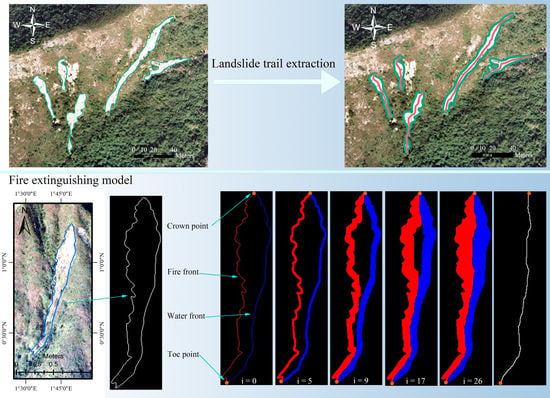
A fire extinguishing model is proposed for centerline extraction from polygonal objects. The model guarantees the centrality of the resulting centerlines while preserving the topology without resorting to branch pruning steps. The main features of this model are its robustness in handling polygons of various shapes and scales, and that it is easy to understand and implement.

(2)

Based on the proposed fire extinguishing model, a new workflow for LTE is implemented, which provides three separate pieces of information about the landslide: the trail, the crown and toe points, and the attributes associated with the trail, such as travel distance, angle, and horizontal distance. The proposed LTE workflow, being stable and fully automatic, is capable of extracting landslide trials that are comparative to manually mapping. This indicates the workflow’s practical value for landslide mapping.

(3)

Experiments from two study areas were carried out based on real-world remote sensing image data, and experimental results demonstrate that the proposed LTE method outperforms the baseline method and can produce better results in terms of completeness, centrality, and direction.

The remainder of this paper is organized as follows: Section 2 reviews the related work on this study, Section 3 presents the new method to extract landslide trails from landslide polygons and digital elevation model (DEM). In Section 4, experiments are performed to validate the effectiveness and superiority of the proposed method. Experiment result discussions and conclusions are given in Section 5 and Section 6, respectively.

2. Related Work

Landslide trails record the flow path of landslide movement. The potential of landslide trial maps has long been recognized and has been used to support a lot of research, but the methods for preparing landslide trail maps have previously received little attention. Although many methods for preparing landslide inventory maps have been developed, the majority of them are polygon- or point-based and little effort has been devoted to the extraction of landslide trails. In the past, LTE was mainly conducted by manual delineation through the interpretation of stereo aerial images [33,34]. Recently, Shi et al. [19] developed a semi-automatic method, which, to the best of our knowledge, is the only existing LTE method.

Since landslide trails are typically represented as centerlines in their flow direction, it is a straightforward strategy to leverage the centerline extraction approaches for LTE. Many centerline extraction applications rely on those skeletonization techniques, which refer to an abstraction process that reduces the dimensionality of an object.

A skeleton provides a simple and compact representation of an object while capturing its major topologic and geometric information. So far, many skeletonization approaches have been proposed, most of which have been successfully applied to object representation. Generally, these approaches share the principle of Blum’s grassfire model [24]. Several review articles summarize skeletonization techniques [28,29,30], providing a systematic comparison of these approaches [30].

The skeletonization approaches can be divided into three categories [29]: (i) geometric approaches [35,36,37,38]; (ii) curve propagation approaches [39,40]; and (iii) digital approaches. Geometric approaches are based on polygonal representations of object boundaries. The skeleton of a polygon can be obtained by taking the intersection points of the polygon and its Voronoi diagram [36]. Curve propagation approaches are based on the principle of the continuous evolution of object boundary curves by which the skeleton is formed at the locations of singularities, e.g., at collision points of opposing boundaries. In digital approaches, the object is represented by a set of pixels in a digital space, and skeletonization is accomplished by iteratively removing boundary pixels through digital morphological erosion or through locating singularities on a digital distance transform (DT) of the digital object. Zhang-Suen’s method [31] is one of the most popular digital approaches due to its fast speed and simplicity [22,41,42].

In general, all of the above methods have the following drawbacks: (i) high sensitivity to small perturbations on the object boundaries [28,43]; (ii) the need for a post-processing procedure for redundant branch pruning [28,43]; and (iii) time-consuming parameter finetuning. Recently, with the popularization of CNNs, deep learning-based methods [25,43,44,45,46,47] have been introduced in an object skeleton detection. These methods, in general, treat skeletonization as a pixelwise classification or a regression problem and produce satisfactory results. However, these methods are inevitably limited, as a large number of well-annotated training samples are needed. Therefore, a skeletonization method for directly generating a satisfying landslide trail from a landslide polygon is still lacking.

Based on skeletonization, in the previous work by Shi et al. [19], Zhang-Suen’s thinning method [31] is employed for LTE. Zhang-Suen’s method produces skeletonized images in two sub-iterations. The first iteration serves to erase boundary points of the south-east and vertex of northwest, while the second iteration serves to erase boundary points of the northwest and vertex of the southeast. This algorithm, being very fast and simple to implement, is one of the most widely used skeletonization algorithms. However, in the case of LTE, it may produce many unwanted branches in the resultant trails. To eliminate this issue, a line simplification process, which serves as pruning, has been subsequently employed in the baseline method. This process can remove redundant branches while also simplifying the extraction results to some extent. However, there were still unresolved issues, including: (i) the skeletonization process is lacking in integration of informative prior knowledge, i.e., topographic information provided by DEM; this may lead to a resulting trail with incorrect direction; (ii) the introduced simplification process is sensitive to the complexity and scale of landslides, which may lead to trails with low centrality; and (iii) the adopted Zhang-Suen’s method, which is under the definition of the grassfire model, can lead to the excessive shrinkage of certain structures [32], causing the problem of incomplete trails. In this study, we address these issues by establishing a fire extinguishing model, i.e., a centerline extraction approach, which is then integrated into the proposed LTE workflow.

3. Method

The proposed method, presented in this paper, takes a digital elevation model (DEM) and mapped landslide polygon data as inputs. Both the input data cover the same geographical extent. By iteratively processing each landslide polygon and outputting a corresponding landslide trail polyline, this method generates a landslide trail map in which each feature represents a landslide trail together with its attributes.

The proposed method for LTE, as shown in Figure 1, mainly consists of three steps:

(1)

Preprocessing. This step is applied to eliminate potential errors in the input data, including (i) Noise reduction for DEM; and (ii) hole filling, topology recovery, and rasterization for a landslide polygon.

(2)

Trail extraction. This is the main procedure for LTE. It consists of three sequential subroutines: (i) Landslide characteristic points localization (LCPL); (ii) Fire extinguishing model (FEM); and (iii) Removal of redundant pixels (RRP). Firstly, two landslide characteristic points, extracted through LCPL, serve as two endpoints for the centerline. Secondly, FEM is proposed to obtain the main body of the centerline. Finally, to guarantee the thinness of the centerline, RRP is used to remove those pixels that cause double-pixel-width.

(3)

Attribute extraction. Landslide trail associated attributes, such as travel distance and vertical drop, are obtained from DEM and the trails.

The detailed process of the above-mentioned steps is explained in the following sections. Specifically, the preprocessing, trail extraction, and attribute extraction stages described in Figure 1 will be elaborated on in Section 3.1, Section 3.2 and Section 3.3. The proposed method will be applied to the mapped landslide data from two study areas in which real landslide events occurred. The related data in the study area will be used to illustrate the processes of the proposed method.

3.1. Preprocessing

The preprocessing module includes (i) denoising for DEM; and (ii) hole filling, topology recovery, and rasterization for mapped polygons. A schematic of the preprocessing is shown in Figure 2.

It is necessary to have the DEM data denoised before it is fed into the next step. DEM is important input data that represent landslide topography, which is highly related to the flow path of landslide materials. Hence, it is essential to guarantee the correctness of DEM. More importantly, the noise in DEM may affect the localization of landslide characteristic points (crown and toe), and the latter is the key input for the subsequent fire extinguishing model, determining the end points of resulting trails. Hence, median filtering, which can effectively remove salt and pepper noise, was applied to DEM using a 3 × 3 window.

As the proposed method is based on landslide polygons for trail extraction, the complexity of polygons itself will affect the complexity of the method. To reduce such complexity, it is necessary to eliminate those errors in landslide polygons prior to further processing. For landslide polygon data, whether it is manually delineated or generated by automatic algorithms, there are usually two types of problem. The first is topological errors, such as self-intersection and cutback vertices; the second, especially for those polygons extracted by automatic algorithms, is holes. The process of eliminating topological errors is referred to as topology recovery, which can be achieved through existing GIS software (e.g., ArcGIS, QGIS). An illustration of polygons with errors and the corresponding recovered ones is shown in Figure 2.

After the above two preprocessing steps, the landslide polygon is transformed into a simple polygon that does not intersect itself and has no holes. Finally, the resultant polygon is rasterized into a binary image representing the landslide object, with the same resolution as DEM. In the landslide object image, a digital number 1 indicates the landslide pixels and 0 indicates the background. An example of polygon rasterization is shown in Figure 2d.

3.2. Landslide Trail Extraction

3.2.1. Landslide Characteristic Point Localization

Often, the endpoints of an object centerline are determined by corner point detection methods, with the most important polygon corner points as endpoints, to avoid redundant branches. The endpoints of the landslide trail, which represent the starting and ending points of landslide movement, are basically independent of the landslide polygon corner points. Instead, it is closely related to the topographic conditions of the landslide, which determine the start and end points of the trail.

In this study, we use two landslide characteristic points, the crown point [48,49] and toe point [48], as the two end points of the landslide centerline. Both points are selected from the landslide polygon boundary. The landslide crown point, which is the start point of the landslide trail, has the highest elevation, while the toe point is the end point and has the lowest elevation. The elevation information of these points can be obtained from DEM. Hence, in this study, the landslide trail is represented as a landslide centerline that starts at the crown point and ends at the toe point.

3.2.2. Fire Extinguishing Model

Before introducing the FEM, we introduced the medial axis definition of skeleton as well as the grassfire model [24]. The FEM proposed is inspired by this model, which provides the earliest definition of the skeleton and describes the process of obtaining a skeleton from an object. Many skeletonization methods are based on such a definition.

• Grassfire model

The grassfire model is proposed by Blum through an analogy of the burning grass process. In this model, an object is assumed to be a dry grass field. Firstly, a fire is simultaneously lit at all boundary points of the grass field. The fire, then, propagates at a uniform speed within the grass field, with quenching points formed at the intersection of two independent fire fronts. Finally, all quenching points together form the skeleton of the object. An example of the grassfire process on a rectangular object is depicted in Figure 3.

In Figure 3, (a) shows the rectangular object, (b) shows the grassfire process, and (c) illustrates the skeleton definition with maximal inscribe disks. The lit point is colored in a red dotted line, and the point where the fire front meets is displayed by an orange dot. Iteration i correspond to the propagation time.

At ignition of the fire (i = 0), the polygon boundary is lit, the fire front is then propagated at simultaneous speed, to the inside of the polygon. The fire propagation process stops at the 5th (i = 5) iteration.

As shown in Figure 3, the grassfire model is a useful tool for converting a landslide polygon into a skeleton. However, such a model suffers from unnecessary branches in the resulting skeleton. During the grassfire process, several redundant branches are created in the resulting skeleton (see Figure 3 (i = 5)). In this study, the resulting landslide trail is preferred to be a simple polyline with no branches. To this end, an improved skeletonization routine, i.e., fire extinguish model, is devised in this research.

2.

Definition of fire extinguishing model

Similar to the skeleton, a centerline of a polygonal object can also be defined by the center locus of maximum inscribed disks of two curves. The latter are the object boundary segments separated by two distinct boundary points. The definition is as follows.

Definition 1.

Let R denote a set which contains all the points in a plane polygon field and ΓR denote the set of its boundary points, suppose the ΓR is split by two distinct boundary points, referred to as endpoints A and B, into two segments, i.e., C_w and C_f. ∀P ∈ R, suppose M denotes the closest point from C_w to P, namely, ∀T ∈ C_w, |PM| < |PT|; and suppose N denotes the closest point from C_f to P, namely, ∀T ∈ C_f, |PN| < |PT|. If |PM| = |PN|, then P is considered a centerline point with endpoints A and B of the plane polygon field R. The set of all skeleton points is the centerline of the plane polygon field R.

To obtain the centerline by this definition, the FEM which depends on the endpoints obtained by LCPL, is proposed. The schematic illustration of FEM on a rectangular polygon is shown in Figure 4.

For ease of description, we describe the proposed FEM by an analogy of extinguishing a grass fire on a hill slope. Specifically, we assume that the object in the binary image is a grass field located on a slope, with the grass field being combustible and the area beyond the grass field being noncombustible. There are two boundary points (denoted as A and B, the two end points) located at the same horizontal level that divide the grass boundary into the upper and lower sides of the slope (see Figure 4b). Assume the grass on the lower boundary (the initial fire front C_f, see Figure 4c) is on fire, and water is poured on the upper side boundary (the initial water front C_w, see Figure 4c) to extinguish the fire. The fire front will gradually propagate uphill as it burns, while the water front will propagate downhill due to gravity.

Assume that water and fire travel at the same speed, and that their propagation is not affected by any other factors unless they reach quench points. A quench point is formed where fire front and water front meet, and the water and fire fronts, at this point, stop propagate. Hence, the first two quench points are A and B, in which the initial fire and water fronts meet. As the water and fire front propagation continues, more quench points emerged; and when all the fire is extinguished, the propagation process stops. All quench points form the centerline of the grass field, i.e., the centerline of the object. In this study, the propagation is implemented through an iterative process, in each iteration, the fire and water front move one step inside the raster object, and each step is of one-pixel length. The whole process can be referred to Figure 4c.

As shown in Figure 4c, i represents the ith iteration (beginning with i = 0) of water and fire propagation. In the first iteration (i = 0), the two end points become quench points because they are at the collision point where the fire front and water front meet. More and more quench points form as the propagation process continues (see Figure 4c i = 1,2,3,4). Finally, once the fire fronts are completely extinguished, all quench points form the object’s centerline (see Figure 4c i = 4).

3.

Difference between the proposed FEM and the grassfire model

Note the proposed method is not a simple reimplementation of the grassfire model, and is substantially different from it. In the grassfire model, each time opposing front-fires collide in the grassfire process, a quench point is created, and a branch would be formed where there is a perturbation at the boundaries. This means that the method is sensitive to boundary noise. This usually causes many meaningless quench points, thus producing spurious skeletal branches. In contrast, in the proposed method, a quench point is generated only when the water front meets the fire front, and no quench point is generated even when the opposite identical fronts meet. The result is that perturbations would not result in new branches. Consequently, the generated centerline is free of unnecessary branches.

3.2.3. Removal of Redundant Pixels

By the above process, a binary image S is obtained, in which pixels with a value of 1 represent the centerline extracted from the object, while pixels with a value of 0 represent the background. Note that the width of the centerline C in S is not the ideal unit-pixel-width; rather, it is at the most double-pixels-wide everywhere, which, however, does not meet the thinness requirement of a landslide trail. This is due to the discrete implementation of FEM. During the fire extinguishing process, the object boundary is partitioned by two endpoints into two curves, corresponding to the initial fire front and water front, respectively. The two initial curves are equally distant from the skeleton point. This may lead to a double-pixel-wide skeleton in those discrete cases, such as when the ideal skeletal points are not located in the center of a pixel but, rather, at the center of two neighboring pixels. These two pixels, one of which is considered redundant, together represent a centerline point, hence resulting in a double-pixel width.

To obtain a centerline with the unit pixel width, we use the 8-connectivity number (C8) [13] to remove redundant pixels in C. The 8-connectivity number, defined as the number of connected components of the neighbor of a pixel, is commonly applied to determine whether the removal of a pixel results in dis-connectivity [50]. For every pixel p in its 8-connectivity neighborhood (see Figure 5), the C8 can be calculated as follows.

$$\mathrm{C}8={\displaystyle \sum }_{k=1}^4\left({\overline{p}}_{2k-1}-{\overline{p}}_{2k-1}·{\overline{p}}_{2k}·{\overline{p}}_{2k+1}\right)$$

(1)

where p_k ∈ {0,1}, $\overline{p_k}$ = 1 − p_k, and p₉ = p₁.

For centerline pixels with unit pixel width, their C8 is 2, while those centerline pixels with double-pixel-width (non-endpoint) have a C8 of 1, and these pixels are called redundant pixels. Hence, the method for the removal operation is as follows: Step 1: Find one redundant pixel and remove it from C; Step 2: Repeat Step 1 until no more changes occur. With such a removal operation, the centerline with a unit-pixel-width is finally generated.

Notably, the removal operation may decrease the centrality of the resulting centerline. After the removal operation, some pixels in the resulting single-pixel-width skeleton C may be shifted by half a pixel width from the true medial axis. However, such a centrality problem is negligible, since the extent of the offset can be limited by controlling the resolution of object discretization in the rasterization step in preprocessing.

In addition to planar two-dimensional (2-D) trails (see Figure 5) as described above, the longitudinal profile of the landslide (profile along the centerline of the landslide), i.e., three-dimensional (3-D) trails (see Figure 5), can also be obtained by our method. This can be easily achieved by assigning an elevation from the DEM to each point in the trail.

An example of a real-world landslide polygon through the proposed LTE method is shown in Figure 6. Figure 6 depicts the landslide in a 3-D view aerial photo, with the landslide boundary marked in blue; (b) depicts the landslide polygon (in white) in a horizontal plane; (c)–(g) depict the fire extinguishing process; and (h) depicts the resulting landslide trail (in white). Figure 6c shows two endpoints determined by LCPL that divide the landslide boundary into two curves, one representing the water front (colored in blue) and the other representing the fire front (colored in red). As the fire and water fronts propagate inside the landslide object (see Figure 6c–g, a skeleton line (see Figure 6h) is formed.

3.3. Landslide Attribute Extraction

Many scenarios in landslide studies require knowledge of the landslide attributes such as travel distance and vertical drop. The landslide attribute is vital in analyzing landslide mechanisms, determining landslide types, and as a preparatory step for susceptibility modeling [51,52,53], hazard mapping [15,54], and indirect assessment of inventory completeness [55].

In this study, five quantitative properties are suggested to characterize landslide trails. Only attributes directly related to landslide trails are calculated. As shown in Figure 7, the five attributes considered are crown point, toe point, horizontal distance, vertical drop, and travel distance. The definitions of these attributes are listed in

Table 1. Landslide characteristic parameters derived from the landslide trail.

Attribute	Denotation	Definition
Crown point	C	A point at the top of the landslide crown (highest point).
Toe point	T	A point at the distal end of debris tail (lowest down slope point).
Vertical drop	H	The vertical height of a landslide, it is equal to the altitude difference between the crown point and the toe point.
Horizontal distance	Lh	The length of the 2-D trail.
Travel distance	Lt	The length of the 3-D trail.
Mobility index	M	The ratio between the vertical drop (H) and the horizontal travel distance (Lh), i.e., H/Lh.
Travel distance angle	A	The angle between the horizontal plane and the line connecting the crown and toe points, equivalent to the arctangent of the mobility index.

.

4. Experiment and Analysis

To demonstrate the effectiveness and superiority of the proposed method, this study used landslide data from a landslide prone area on Lantau Island in Hong Kong to carry out LTE experiments. In this section, the experimental setup, including methods for comparison and the experimental data from two study areas, is first described. Next, the quantitative evaluation method used in this experiment is explained in detail. Finally, the qualitative and quantitative comparisons of the landslide trail extraction results are carried out. The details of each part are as follows.

4.1. Experimental Setup

To evaluate the approach proposed in this study, the baseline method is used for comparison. In addition, one of the most popular skeletonization methods, i.e., the Zhang-Suen method, is used to demonstrate the issue with skeletonization for LTE. Zhang-Suen’s method can be seen as an implementation of the grassfire model, while the baseline method is, to the best of our knowledge, the only existing LTE method.

4.1.1. Study Area

In this study, two landslide-intensive sites, namely A and B, on Lantau Island in Hong Kong, China, are selected as study areas (see Figure 8a). Lantau Island is an outlying island featuring steep terrains. On 7 June 2008, a severe rainstorm affected the whole of Hong Kong, causing over 2400 landslides in the western part of Lantau Island [56]. It is reported that the total rainfall reached 307.1 mm within 24 h. The landslides present various shapes and scales, with many of them traveled long distances [57]. The aerial photo for study areas A and B are shown in Figure 8b,c, respectively.

4.1.2. Dataset

The aerial image and DEM of the study area are used to demonstrate the effectiveness of the proposed method. For both study areas, the DEM was made from airborne LiDAR data in 2010, with a spatial resolution of 0.5 m/pixel. By comparing the landslide features in aerial photos taken in November 2008 (approximately 4 months after the landslide occurrence) with the hill-shade image of DEM, we confirmed that, in landslide affected areas, terrain features from DEM were consistent with spectral features in aerial photos. As an example, Figure 9 shows the validity of DEM. Thus, no large-scale topographic changes occurred in landslide areas during this period.

The aerial images used for visual analysis in the two areas were acquired by using a Zeiss RMKTOP 15 Aerial Survey Camera at a flying height of approximately 2400 m in November 2011. The spatial resolution of the aerial photos is 0.5 m/pixel, and it was geometrically and radiometrically corrected by the Hong Kong Civil Engineering and Development Department (CEDD).

To extensively validate the robustness of the proposed method, the landslide polygons in two regions, extracted by manual mapping and an automated algorithm, respectively, are chosen for experiments. For study area A, an inventory dataset of the polygons of the landslides was prepared from a manual delineation of landslides based on the aerial imagery. A total of 20 landslide events were mapped as polygons. The landslide polygon in this area is relatively simple and the boundary is relatively smooth, but some of the landslide polygons have topological errors. For a fair comparison, all the landslide polygons are pre-processed in advance to eliminate topological errors.

For study area B, the landslide polygons are generated by a state-of-the-art landslide detection algorithm [19]. The number of landslides obtained is 88. Those landslide polygons are more complex. Some polygons contain holes (e.g., Figure 10a) and some are incomplete (e.g., Figure 10b). The hole issue is caused by the complex nature of landslides and the limits of automated algorithms. After a landslide event, the affected area is generally eroded into bare land, which consequently contrasts with the surrounding area. A landslide polygon map can be well-prepared by identifying such a contrast. However, during a landslide event, vegetation may move together with the landslide materials and not be eroded. In this case, the vegetation area inside the landslide does not become bare land and presents a similar characteristic to the surrounding area of the landslide. As a result, it is represented as holes in a landslide polygon (see Figure 10a). Besides, due to the recovery of vegetation, some landslide polygons are incomplete (see Figure 10b). Finally, the extracted landslide edges may not be smooth. Instead, they are serrated because this area is geographically matched with raster pixels in aerial imagery.

For both areas, the prepared landslide inventory dataset was visually verified using the available ENTLI records and aerial imagery. All erroneous landslide polygons were removed. Finally, the ground truth for landslide trails of the two areas is manually delineated by referring to ENTLI and landslide polygon.

4.1.3. Evaluation Metrics

To quantitatively evaluate the proposed LTE method, the first step is to determine the correctness of the extracted landslide trails. However, it remains an unsolved problem of how to quantitatively compare the extracted trail with the reference trail, as the validation of skeletonization algorithms is still a challenging issue [29]. Specifically, the landslide trail is a geometric feature of a landslide and is essentially invisible to the naked eye. This means that given a landslide polygon, no cartographer can manually delineate a landslide trail as the ground truth, which is perfectly centered inside the landslide polygon. Hence, conventional evaluation methods, which measure everything at pixel levels [58], are not suitable for the trail similarity comparison in this experiment.

In this study, we adopted an IoU-based line similarity measurement method, which allows small localization errors, to assess the quality of LTE results. The process of similarity measuring between trails can be seen in Figure 11. As can be seen from Figure 11, the buffer polygon, instead of the original trail polyline, is used for evaluation. Specifically, the trail is first buffered with certain buffer distances (which can also be referred to as tolerance) into a polygon (see Figure 11a), and this polygon is then used to substitute the original trail to enable a comparison. By comparing the similarities of the two polygons, the correctness of the extracted trails can be determined.

In this experiment, four buffer distances ranging from 0.5 m to 2 m were employed. Moreover, the widely used evaluation metric, i.e., intersection over union (IoU), which measures similarity between two polygons, is employed as the evaluation metric for the two buffer polygons. The IoU is calculated as follows:

$$\mathrm{IoU}=\frac{ \mathrm{Intersection} }{ \mathrm{Union} }$$

(2)

where Intersection means “the area of intersection” between two polygons, while the Union represents “the area of union” between the two polygons. To determine if the two polygons are consistent, a threshold was used. When the IOU between two polygons is greater than this threshold, and the corresponding two trails are considered to be consistent, the resulting trail is thus considered to be correct; otherwise, the resulting trail is regarded, incorrect. In this manner, the landslide trails extracted by the proposed method can be compared with manually edit reference trails. Finally, the widely used precision index is employed to calculate the ratio of correctly extracted trails. The definition of Precision is as follows:

$$\mathrm{Precision} =\frac{N_1}{N}$$

(3)

where N₁ is the number of trails that are correctly extracted; N is the number of all landslides in the study area.

4.2. Results and Qualitative Evaluation

4.2.1. Study Area A

The results of the landslide trail map obtained in study area A are shown in Figure 12. In Figure 12a,b are the landslide polygons overlaid on the aerial image and DEM, respectively. The ground truth of the landslide trail is presented in Figure 12c. The LTE results by methods of Zhang-Suen, baseline, and the proposed are shown in Figure 12d–f, respectively. For better visual performance, all trails are superimposed with landslide polygons, and to show the topography of the landslide area, they are overlaid on DEM. Different colors are used in the figure to display the trail results, where yellow indicates correct results, while other colors indicate results with problems (please refer to the figure legend for the specific meaning).

As shown in Figure 12, all methods can simplify the landslide polygons into polylines effectively due to the use of the skeletonization tools. However, as far as landslide trails are concerned, some results by skeletonization are not correct. As can be seen in Figure 12d, the results marked in purple indicate that the direct use of Zhang-Suen’s method results in redundant branches; this issue is fixed in the baseline method, no results with redundant branches were found (Figure 12e); however, the results by baseline method have other problems, for example, some result trails are not centered inside the landslide polygon (see Figure 12e red results), and some results are incomplete as they are too short to represent the landslide flow path (see Figure 12e blue results). In contrast, all results by the proposed method are marked in yellow, hence indicating that all of the results are correct. This implies that although there are landslides of various shapes, the proposed method produces the most favorable results.

A region, as shown in Figure 12a in a red rectangle, is magnified and is shown in Figure 13 for a more detailed analysis. This region contains landslides of various shapes. Some landslides have branches, and some contain very narrow sliding paths. In Figure 13a,b are the landslide polygons overlaid on aerial images and DEMs, respectively. The ground truth of the landslide trail is presented in Figure 13c. The LTE results by the methods of Zhang-Suen, baseline, and the proposed are shown in Figure 13d–f, respectively.

As shown in Figure 13d, spurious branches (colored in purple) can be found in all of the trails obtained by Zhang-Suen’s method, lowering the quality of the resulting trail maps. This is due to the inherent characteristics of the grassfire model, which produces an additional branch for each curvature extreme point in a polygon.

In contrast, no purple results were found in the baseline method results, as shown in Figure 13e. This is due to the simplification process introduced after the skeletonization, in which those unwanted branches are removed while the resulting polyline is simplified. However, the simplification process may result in a poor centrality of landslide trails due to oversimplification, as indicated by the red results in Figure 13e.

In comparison to the baseline method, the proposed methods, as shown in Figure 13f, produce a more consistent result to the reference trail, with the resulting trail not only being centered inside the landslide boundary, but also being free of spurious branches. All the trails obtained by the proposed method basically follow the sliding direction of the landslide. This is because the proposed method chooses the crown and toe point as the two endpoints of the resulting skeleton, thus allowing the landslide trail to retain the correct sliding direction. This demonstrates the robustness of this paper’s proposed method.

4.2.2. Study Area B

The results for study area B are shown in Figure 14, in which (a) is the landslide polygon which overlies an aerial image, red boxes in (a) indicate regions that will be magnified, which is shown, and is further discussed in detail later in this section. The ground truth of the landslide trail is presented in (b). Figure 14c,d show the LTE results using the baseline and proposed methods, respectively. Different colors are used in the resulting figure to display the trail extraction results. The color yellow indicates the correct extraction results, while other colors indicate results with problems (please refer to the figure legend for the specific meaning). As demonstrated in the result for area A, the landslide trails extracted by Zhang-Suen’s method suffer from redundant branches. They are not suitable for LTE and are thus not further evaluated in study area B.

The proposed method produces more yellow results than the baseline method, as shown in Figure 14c,d, indicating that it outperforms the baseline method. This is mainly due to the fact that it takes advantage of both the geometric and topological information contained in landslides. In contrast to the proposed method, the baseline method produces results with flaws such as poor centrality (see Figure 14c red results) and incompleteness (see Figure 14c blue results).

To further demonstrate the effectiveness and superiority of the proposed method, eight representative regions marked with red boxes in Figure 14 are selected to zoom into, in order to gain a closer look at the performance of the trail extraction for landslides with various shapes and topographies. The results are displayed in Figure 15. The first and fourth columns contain the landslide polygon overlaid on aerial imagery. The results by the baseline and proposed method are superimposed on the landslide polygon and DEM and are shown in the second and fifth columns, and on the third and sixth columns, respectively.

To address the redundant branches issue, the baseline method introduces a simplification process, which removes unwanted branches. In the meantime, it simplifies the resulting trails to some extent. However, due to the diversity of landslide scales and shapes, the simplification process is not robust enough to maintain the correctness of all trails. This may cause two problems for the resulting trails. One problem is the low centrality of the trails. As indicated by the red results in Figure 15b,e,h,q, those results are not centered inside the landslide polygon, and there are even results with parts that lie outside the landslide extent (see Figure 15h).

Another problem is the incompleteness of the resulting landslide trails, such as the blue results shown in Figure 15k,t,w. This is due to the excessive erosion [59] caused by Zhang-Suen’s method. During the two-iteration process in Zhang-Suen’s method, the outer pixels are removed, and for some nearly circular, oriented regions, the skeleton shrinks considerably, even leading to the disappearance of some structures [32,59], as shown in Figure 15h.

Finally, as shown in the orange trails in Figure 15n, the results extracted by the baseline method suffer from the problem of wrong directions. Because only geometric information is considered during the LTE process, it may result in trails with the wrong directions, especially when the longitudinal direction of the landslide geometry is not consistent with the landslide movement direction.

In contrast, the proposed method, as shown in the third and last columns, obtains the highest number of correct results. The resulting trail not only preserves the direction of the original landslide but is also free from spurious branches. Furthermore, the results preserve good centrality even when there are holes in the landslide polygon (see Figure 15b,e), thanks to the preprocessing step that removes inner holes first. However, as shown by the red results in Figure 15o, there are also incorrect trails. This is due to the spectral heterogeneity. The landslide is wrongly identified by the automated algorithm as two distinct ones, leading to the problem that the extracted trails also have unsatisfied centrality. Despite this, the overall direction (northeast to southwest) of the two separated landslide trails remains approximately correct and consistent. This is indicative of the contribution of the incorporation of topographic information in the proposed method. As such, the proposed method can be deemed effective in complex scenarios.

4.3. Quantitative Evaluation

For quantitative evaluation, the LTE results of the proposed and baseline methods are compared with the reference landslide trails (ground truth) using the previously mentioned line similarity measurement metrics. Four buffer distances ranging from 0.5 m to 2.0 m, and the precision under different IOU thresholds, is used to illustrate the performance of the proposed method. The precision curves for two study areas are illustrated in Figure 16 and Figure 17, respectively. The numerical results under two IoU thresholds (0.3 and 0.5) are presented in

Table 2. Evaluation results for landslide trail extraction in study area A, bold denotes the best results for each measurement.

Buffer Distance (m)	Threshold	Precision
		Baseline	Proposed
0.5	0.3	0.60	0.90
	0.5	0.15	0.35
1.0	0.3	0.85	1.00
	0.5	0.60	0.90
1.5	0.3	0.95	1.00
	0.5	0.70	1.00
2.0	0.3	0.95	1.00
	0.5	0.80	1.00

and

Table 3. Evaluation results for landslide trail extraction in study area B, bold denotes the best results for each measurement.

Buffer Distance (m)	Threshold	Precision
		Baseline	Proposed
0.5	0.3	0.26	0.64
	0.5	0.01	0.20
1.0	0.3	0.64	0.95
	0.5	0.27	0.70
1.5	0.3	0.85	0.99
	0.5	0.44	0.84
2.0	0.3	0.95	1.00
	0.5	0.59	0.93

, respectively.

As shown in Figure 16 and Figure 17, the proposed method overwhelmingly outperforms the baseline method in terms of precision under all four-buffer distances. In addition, as shown in Table 2 and Table 3, when the buffer distance is set greater than 1.0 m, for study area A, the precision is over 0.9 (IoU = 0.5), and for study area B, the precision is over 0.7 (IoU = 0.5), indicating that most landslide trails are correctly extracted by the proposed method.

In summary, the proposed method achieves a much better precision than the baseline method. Hence, the quantitative comparisons have clearly demonstrated and supported the effectiveness and superiority of the proposed method. Combined with visual observations and quantitative analysis in the two study areas, the proposed method achieves favorable LTE results. In both study areas, no spurious branches are generated in the resulting landslide trail obtained by the proposed method. Because the geographic information is considered during the skeletonization process, end points are determined before the skeletonization process, and as a result, meaningless endpoints are avoided. In addition, a fire extinguishing process is implemented, which guarantees the centrality of the LTE results.

5. Discussion

In the experiments, two landslide-prone areas in Hong Kong are selected to valid the effectiveness of the proposed LTE workflow. However, the proposed workflow can be applied readily to other areas with different landslide scale, shapes, materials and types, as the method does not depend on remote sensing images as inputs; instead, it uses well-prepared landslide polygon maps as an input, which avoids the uncertainties brought about in remote sensing images. Moreover, the preprocessing step further reduces the uncertainties in manually induced errors. Due to the complex nature in remote sensing images, the landslide polygon map produced by manual delineation or automated programs may still contain topology errors, such as cutback vertices and self-intersection. Thus, there may still exist uncertainties in landslide polygon maps. With a preprocessing sub-routine in the proposed workflow, robustness could be further guaranteed. Detailed discussions on the computational complexity, advantage, limitations and future work are as described below.

5.1. Computational Complexity

The computation process of the proposed LTE method is comprised of three major components: (a) Landslide characteristic point localization; (b) Fire extinguishing model; and (c) Removal of redundant pixels. With raw LiDAR data preprocessed to DEM, all the experiments are performed with C++ on a computer with Intel Core i7-8550U CPU@ 2.50 GHz and 16.0 GB RAM. The most time-consuming part is the fire extinguishing process, since this requires it to iteratively update the state of fire and water fronts in a rasterized binary object, and the computation time mainly depends on the scale of the landslide polygons. To check the efficiency of the proposed method, the computation time of the method applied to the two study areas are recorded, the detail of the processing time is shown in

Table 4. Computational complexity analysis of the proposed method.

Study Area	Running Time (Seconds)
	Baseline	Proposed
A	3	9
B	10	18

.

Table 4 has 2 rows and 3 columns. The first column shows the study area. The second and the third column are the running time for the baseline method and the proposed method, respectively. It can be seen from Table 4 that the proposed method runs slower than the baseline method in both study areas; this is due to the multiple iterations of the fire extinguishing process, where the process would not stop until every fire pixel is extinguished. However, the baseline method requires an iteratively parameter adjustment, which is time-consuming and is not favorable in a practical environment. Moreover, the time for parameter adjustment is hard to evaluate. Table 4 also shows that as the complexity of landslide polygons increase (from study area A to study area B), the running time of the baseline method (from 3 s to 10 s, a 3-fold increase) varies greater than that of the proposed method (from 9 s to 18 s, a 2-fold increase), indicating that the proposed method is more robust to the complexities of landslide shape and scales.

5.2. Advantages

The effectiveness and robustness of the proposed method have been qualitatively and quantitatively validated. Compared with the baseline method, the proposed method is capable of generating landslide trails that are free from spurious branches, directional errors, incompleteness, and poor centralities. Moreover, it has the following appealing advantages:

• It is an automatic LTE method. It combines topological and geometric information of landslides effectively. Thus, it can reduce the load on users substantially.
• In addition to the geometric information, it also considers the topological information of landslides, allowing it to generate landslide trails more accurately.
• There are no parameter finetuning requirements, unlike the baseline method, which requires two free parameters. As a result, it would be more practical in real-world applications.

Finally, it has one additional appealing characteristic. The prerequisite for the proposed LTE method is that the landslide polygon should be prepared in advance. To date, there are several techniques available to automatically identify landslides from remote sensing imagery (e.g., [60,61,62]) and various methods to delineate the landslide polygon, such as deformable model-based methods [63], object-based methods [64], and deep learning-based methods [19,60]. Any of these methods can be conveniently integrated into the proposed method. Despite the hole issues being common inside landslide polygons obtained by these methods, our method can extract trails accurately.

One may note that the localization of the crown and toe points may affect the results of trail extraction. However, the influence is limited owing to the adoption of a median filter in the preprocessing step for DEM, which can avoid salt-noise in DEM and thus enables the presented method to be sufficiently robust with regards to the interference of noise in the landslide polygons.

5.3. Limitations and Future Work

One limitation of the proposed LTE lies in its dependence on well-prepared landslide polygons. Roughly produced landslide polygons (such as being incomplete), especially those produced by automated algorithms, may lead to incorrectness in the resulting trails.

Given that manual mapping from remote sensing images is time-consuming and that automated landslide boundary mapping programs may further introduce errors to the resulting landslide polygons, it would be interesting to extract landslide trails directly from remote sensing images. This also alleviates the dependence of the proposed method on well prepared landslide polygons. In recent years, machine learning methods are often used to extract objects from remote sensing data and achieved considerable results. Therefore, using machine learning methods to extract landslide trails is more promising. Notably, although producing the ground truth of training samples is labor-intensive and tedious for supervised learning paradigms, the proposed method could be applied to obtain landslide trails which serve as ground truth data for training samples of machine learning-based methods. Therefore, in future work, attention can be paid to employing machine-learning methods to produce landslide trail maps from remote sensing data.

6. Conclusions

This study has presented a novel and automatic workflow for LTE from landslide polygon maps and DEM, and achieves an LTE that is comparable to human raters. The employment of the proposed FEM enables the generation of landslide trails without redundant branches. More importantly, compared with the baseline method, the proposed LTE workflow can generate landslide trails with better centrality, completeness, and a correct direction. Combined with landslide attribute extraction, the comprehensive LTE workflow can accurately produce landslide trail maps from existing landslide polygon maps. Through tests on landslide polygons with various shapes and scales from two study areas, the effectiveness and superiority of the proposed LTE workflow have been demonstrated. Notably, the method has shown its capability of generating landslide trails from landslide polygons obtained by automated algorithms. In this sense, less demand is placed on either collecting new landslide polygon data or carefully collecting data, particularly during emergency hours, hence helping to reduce the long-term surveying costs for landslide disaster administrators or emergency managers.

References

1. Dai, F.C.; Lee, C.F.; Wang, S.J. Characterization of Rainfall-Induced Landslides. Int. J. Remote Sens. 2003, 24, 4817–4834. [Google Scholar] [CrossRef]
2. Gao, L.; Zhang, L.; Lu, M. Characterizing the Spatial Variations and Correlations of Large Rainstorms for Landslide Study. Hydrol. Earth Syst. Sci. 2017, 21, 4573–4589. [Google Scholar] [CrossRef] [Green Version]
3. Nugraha, H.; Wacano, D.; Dipayana, G.A.; Cahyadi, A.; Mutaqin, B.W.; Larasati, A. Geomorphometric Characteristics of Landslides in the Tinalah Watershed, Menoreh Mountains, Yogyakarta, Indonesia. Procedia Environ. Sci. 2015, 28, 578–586. [Google Scholar] [CrossRef] [Green Version]
4. Kang, C.; Zhang, F.; Pan, F.; Peng, J.; Wu, W. Characteristics and Dynamic Runout Analyses of 1983 Saleshan Lan slide. Eng. Geol. 2018, 243, 181–195. [Google Scholar] [CrossRef]
5. Franks, C.A.M. Characteristics of Some Rainfall-Induced Landslides on Natural Slopes, Lantau Island, Hong Kong. Q. J. Eng. Geol. Hydrogeol. 1999, 32, 247–259. [Google Scholar] [CrossRef]
6. Sun, Y.; Yang, J.; Song, E. Runout Analysis of Landslides Using Material Point Method. In IOP Conference Series: Earth and Environmental Science; IOP Publishing: Bristol, UK, 2015; Volume 26, p. 12014. [Google Scholar] [CrossRef] [Green Version]
7. McDougall, S. 2014 Canadian Geotechnical Colloquium: Landslide Runout Analysis—Current Practice and Challenges. Can. Geotech. J. 2017, 54, 605–620. [Google Scholar] [CrossRef] [Green Version]
8. Finlay, P.J.; Mostyn, G.R.; Fell, R. Landslide Risk Assessment: Prediction of Travel Distance. Can. Geotech. J. 1999, 36, 556–562. [Google Scholar] [CrossRef]
9. Cruden, D.M.; Fell, R. (Eds.) Landslide Risk Assessment; Routledge: Oxfordshire, UK, 2018; ISBN 978-0-203-74952-4. [Google Scholar]
10. Hungr, O. A review of landslide hazard and risk assessment methodology. Landslides Eng. Slopes. Exp. Theory Pract. 2016, 1, 3–27. [Google Scholar] [CrossRef]
11. Ho, K.K.S.; Ko, F.W.Y. Application of Quantified Risk Analysis in Land-slide Risk Management Practice: Hong Kong Experience. Georisk 2009, 3, 134–146. [Google Scholar] [CrossRef]
12. Kwan, J.S.H.; Chan, S.L.; Cheuk, J.C.Y.; Koo, R.C.H. A Case Study on an Open Hillside Landslide Impacting on a Flexible Rockfall Barrier at Jordan Valley, Hong Kong. Landslides 2014, 11, 1037–1050. [Google Scholar] [CrossRef]
13. Ng, K.C.; Chiu, K.M.; Ho, K.K.S.; Chan, V.M.C. Application of GIS to Landslide Risk Management in Hong Kong. In Proceedings of the 2008 Géo Edmonton2008, Edmonton, AB, Canada, 21–24 September 2008; pp. 434–441. [Google Scholar]
14. Lo, C.-M.; Feng, Z.-Y.; Chang, K.-T. Landslide Hazard Zoning Based on Numerical Simulation and Hazard Assessment. Geomat. Nat. Hazards Risk 2018, 9, 368–388. [Google Scholar] [CrossRef] [Green Version]
15. Dahal, R.K. Landslide Hazard Mapping in GIS. J. Nepal Geol. Soc. 2017, 53, 63–91. [Google Scholar] [CrossRef]
16. Ma, Z.; Mei, G. Deep Learning for Geological Hazards Analysis: Data, Models, Applications, and Opportunities. Earth Sci. Rev. 2021, 223, 103858. [Google Scholar] [CrossRef]
17. Kwan, J.S.H.; Koo, R.C.H.; Ng, C.W.W. Landslide Mobility Analysis for Design of Multiple Debris-Resisting Barriers. Can. Geotech. J. 2015, 52, 1345–1359. [Google Scholar] [CrossRef]
18. Venture, M.F.J. Final Report on the Compilation of the Enhanced Natural Terrain Landslide Inventory; HKSAR Government, Geotechnical Engineering Office: Kowloon, Hong Kong, China, 2007.
19. Shi, W.; Zhang, M.; Ke, H.; Fang, X.; Zhan, Z.; Chen, S. Landslide Recognition by Deep Convolutional Neural Network and Change Detection. IEEE Trans. Geosci. Remote Sens. 2020, 59, 4654–4672. [Google Scholar] [CrossRef]
20. Cheng, G.; Zhu, F.; Xiang, S.; Pan, C. Road Centerline Extraction via Semisupervised Segmentation and Multidirection Nonmaximum Suppression. IEEE Geosci. Remote Sens. Lett. 2016, 13, 545–549. [Google Scholar] [CrossRef]
21. Miao, Z.; Shi, W.; Zhang, H.; Wang, X. Road Centerline Extraction from High-Resolution Imagery Based on Shape Features and Multivariate Adaptive Regression Splines. IEEE Geosci. Remote Sens. Lett. 2013, 10, 583–587. [Google Scholar] [CrossRef]
22. Luthra, R.; Goyal, G. Simulation of Zhang Suen Algorithm Using Feed-Forward Neural Networks. Commun. Appl. Electron. 2015, 2, 9–15. [Google Scholar] [CrossRef] [Green Version]
23. Wieser, E.; Seidl, M.; Zeppelzauer, M. A Study on Skeletonization of Complex Petroglyph Shapes. Multimed. Tools Appl. 2017, 76, 8285–8303. [Google Scholar] [CrossRef] [Green Version]
24. Blum, H. A Transformation for Extracting New Descriptors of Shape; MIT Press: Cambridge, UK, 1967. [Google Scholar]
25. Wang, T.-Q.; Liu, C. Fully Convolutional Network Based Skeletonization for Handwritten Chinese Characters. In Proceedings of the Thirty-Second AAAI Conference of Artificial Intelligence, New Orleans, LA, USA, 2–7 February 2018. [Google Scholar]
26. Zhao, F.; Tang, X. Preprocessing and Postprocessing for Skeleton-Based Fingerprint Minutiae Extraction. Pattern Recognit. 2007, 40, 1270–1281. [Google Scholar] [CrossRef]
27. Mliki, H.; Zaafouri, R.; Hammami, M. Human Action Recognition Based on Discriminant Body Regions Selection. Signal Image Video Process. 2018, 12, 845–852. [Google Scholar] [CrossRef]
28. Saha, P.K.; Borgefors, G.; Di Baja, G.S. Skeletonization and Its Applications—A Review. In Skeletonization; Elsevier: Amsterdam, The Netherlands, 2017; pp. 3–42. [Google Scholar]
29. Saha, P.K.; Borgefors, G.; Di Sanniti Baja, G. A Survey on Skeletonization Algorithms and Their Applications. Pattern Recognit. Lett. 2016, 76, 3–12. [Google Scholar] [CrossRef]
30. Siddiqi, K.; Pizer, S. Medial Representations: Mathematics, Algorithms and Applications; Springer Science & Business Media: Berlin/Heidelberg, Germany, 2008; ISBN 140208658X. [Google Scholar]
31. Zhang, T.; Suen, C. A Fast Parallel Algorithm for Thinning Digital Patterns. Commun. ACM 1984, 27, 236–239. [Google Scholar] [CrossRef]
32. Lü, H.E.; Wang, P.S.P. A Comment on a “Fast Parallel Algorithm for Thinning Digital Patterns”. Commun. ACM 1986, 29, 239–242. [Google Scholar] [CrossRef]
33. Dias, A.; Hart, J.R.; Fung, E.K.S. The Enhanced Natural Terrain Landslide Inventory. In Proceedings of the Natural Hillsides: Study and Risk Mitigation Measures, Proceedings of the Hong Kong Institution of Civil Engineers, Geotechnical Division, Annual Conference, Hong Kong, China, 17 April 2009; Volume 17, pp. 71–78. [Google Scholar]
34. Ho, K.K.S.; Wong, H.N. Application of Quantitative Risk Assessment in Landslide Risk Management in Hong Kong. In Proceedings of the 14th South East Asian Geotechnical Conference, Hong Kong, China, 10–14 December 2001; Volume 1, pp. 123–128. [Google Scholar]
35. Attali, D.; Montanvert, A. Computing and Simplifying 2D and 3D Continuous Skeletons. Comput. Vis. Image Underst. 1997, 67, 261–273. [Google Scholar] [CrossRef]
36. Brandt, J.W.; Algazi, V.R. Continuous Skeleton Computation by Voronoi Diagram. CVGIP Image Underst. 1992, 55, 329–338. [Google Scholar] [CrossRef]
37. Dey, T.K.; Zhao, W. Approximating the Medial Axis from the Voronoi Diagram with a Convergence Guarantee. Algorithmica 2004, 38, 179–200. [Google Scholar] [CrossRef]
38. Liu, H.; Wu, Z.; Frank Hsu, D.; Peterson, B.S.; Xu, D. On the Generation and Pruning of Skeletons Using Generalized Voronoi Diagrams. Pattern Recognit. Lett. 2012, 33, 2113–2119. [Google Scholar] [CrossRef]
39. Dimitrov, P.; Damon, J.N.; Siddiqi, K. Flux Invariants for Shape. In Proceedings of the 2003 IEEE Conference on Computer Vision and Pattern Recognition, Madison, WI, USA, 18–20 June 2003; pp. I-835–I-841. [Google Scholar]
40. Tek, H. Symmetry Maps of Free-Form Curve Segments via Wave Propagation. Int. J. Comput. Vis. 2003, 54, 35–81. [Google Scholar] [CrossRef]
41. Padole, G.V.; Pokle, S.B. New Iterative Algorithms for Thinning Binary Images. In Proceedings of the 2010 3rd International Conference on Emerging Trends in Engineering and Technology, Washington, DC, USA, 19–21 November 2010; pp. 166–171. [Google Scholar]
42. Soni, S.; Kaur, S. To Propose an Improvement in Zhang-Suen Algorithm for Image Thinning in Image Processing. Int. J. Sci. Technol. Eng. 2016, 3, 7481. [Google Scholar]
43. Panichev, O.; Voloshyna, A. U-Net Based Convolutional Neural Network for Skeleton Extraction. In Proceedings of the IEEE/CVF Conference on Computer Vision and Pattern Recognition Workshops, Long Beach, CA, USA, 16–17 June 2019. [Google Scholar]
44. Fodor, Á.; Fóthi, Á.; Kopácsi, L.; Somfai, E.; Lorincz, A. Skeletonization Combined with Deep Neural Networks for Superpixel Temporal Propagation. In Proceedings of the 2019 International Joint Conference on Neural Networks (IJCNN), Budapest, Hungary, 14–19 July 2019; pp. 1–7. [Google Scholar]
45. Jerripothula, K.R.; Cai, J.; Lu, J.; Yuan, J. Image Co-Skeletonization via Co-Segmentation. IEEE Trans. Image Process. 2021, 30, 2784–2797. [Google Scholar] [CrossRef] [PubMed]
46. Ko, D.H.; Hassan, A.U.; Majeed, S.; Choi, J. SkelGAN: A Font Image Skeletonization Method. J. Inf. Process. Syst. 2021, 17, 1–13. [Google Scholar]
47. Wang, C.; Hayashi, Y.; Oda, M.; Itoh, H.; Kitasaka, T.; Frangi, A.F.; Mori, K. Tubular Structure Segmentation Using Spatial Fully Connected Network with Radial Distance Loss for 3D Medical Images. In Proceedings of the International Conference on Medical Image Computing and Computer-Assisted Intervention, Shenzhen, China, 13–17 October 2019; pp. 348–356. [Google Scholar]
48. Dellow, S.; Massey, C.; Cox, S.; Archibald, G.; Begg, J.; Bruce, Z.; Carey, J.; Davidson, J.; Pasqua, F.D.; Glassey, P.; et al. Landslides Caused by the Mw7.8 Kaikōura Earthquake and the Immediate Response. Bull. N. Z. Soc. Earthq. Eng. 2017, 50, 106–116. [Google Scholar] [CrossRef] [Green Version]
49. Pourghasemi, H.R.; Kornejady, A.; Kerle, N.; Shabani, F. Investigating the Effects of Different Landslide Positioning Techniques, Landslide Parti-tioning Approaches, and Presence-Absence Balances on Landslide Susceptibility Mapping. Catena 2020, 187, 104364. [Google Scholar] [CrossRef]
50. Arcelli, C.; Di Baja, G.S. A Width-Independent Fast Thinning Algorithm. IEEE Trans. Pattern Anal. Mach. Intell. 1985, 7, 463–474. [Google Scholar] [CrossRef] [PubMed]
51. Azarafza, M.M.; Azarafza, M.M.; Akgün, H.; Atkinson, P.M.; Derakhshani, R. Deep Learning-Based Landslide Susceptibility Mapping. Sci. Rep. 2021, 11, 24112. [Google Scholar] [CrossRef] [PubMed]
52. Wang, H.; Zhang, L.; Luo, H.; He, J.; Cheung, R.W.M. {{AI-Powered}} Landslide Susceptibility Assessment in Hong Kong. Eng. Geol. 2021, 288, 106103. [Google Scholar] [CrossRef]
53. Wang, Y.; Fang, Z.; Wang, M.; Peng, L.; Hong, H. Comparative Study of Landslide Susceptibility Mapping with Different Recurrent Neural Networks. Comput. Geosci. 2020, 138, 104445. [Google Scholar] [CrossRef]
54. Segoni, S.; Tofani, V.; Rosi, A.; Catani, F.; Casagli, N. Combination of Rainfall Thresholds and Susceptibility Maps for Dynamic Landslide Hazard Assessment at Regional Scale. Front. Earth Sci. 2018, 6, 85. [Google Scholar] [CrossRef] [Green Version]
55. Golovko, D.; Roessner, S.; Behling, R.; Kleinschmit, B. Automated Derivation and Spatio-Temporal Analysis of Landslide Properties in Southern Kyrgyzstan. Nat. Hazards 2017, 85, 1461–1488. [Google Scholar] [CrossRef]
56. Choi, K.Y.; Cheung, R.W.M. Landslide Disaster Prevention and Mitigation through Works in Hong Kong. J. Rock Mech. Geotech. Eng. 2013, 5, 354–365. [Google Scholar] [CrossRef] [Green Version]
57. Su, Z.; Chow, J.K.; Tan, P.S.; Wu, J.; Ho, Y.K.; Wang, Y.-H. Deep Convolutional Neural Network—Based Pixel-Wise Landslide Inventory Mapping. Landslides 2021, 18, 1421–1443. [Google Scholar] [CrossRef]
58. Gao, F.; Wei, G.; Xin, S.; Gao, S.; Zhou, Y. 2d Skeleton Extraction Based on Heat Equation. Comput. Gr. 2018, 74, 99–108. [Google Scholar] [CrossRef]
59. Haseena, F.; Clara, R. Performance Analysis of Iterative Thinning Methods Using Zhang Suen and Stentiford Algorithm. In Proceedings of the International Conference on Advancements in Computing Technologies, Panipat, India, 17–18 February 2018; Volume 4. [Google Scholar]
60. Lv, Z.; Liu, T.; Benediktsson, J.A. Object-Oriented Key Point Vector Dis-tance for Binary Land Cover Change Detection Using VHR Remote Sensing Images. IEEE Trans. Geosci. Remote Sens. 2020, 58, 6524–6533. [Google Scholar] [CrossRef]
61. Prakash, N.; Manconi, A.; Loew, S. A New Strategy to Map Landslides with a Generalized Convolutional Neural Network. Sci. Rep. 2021, 11, 9722. [Google Scholar] [CrossRef]
62. Zhang, A.; Shi, W. Mining Significant Fuzzy Association Rules with Dif-ferential Evolution Algorithm. Appl. Soft Comput. 2020, 97, 105518. [Google Scholar] [CrossRef]
63. Li, Z.; Shi, W.; Myint, S.W.; Lu, P.; Wang, Q. Semi-Automated Landslide Inventory Mapping from Bitemporal Aerial Photographs Using Change Detection and Level Set Method. Remote Sens. Environ. 2016, 175, 215–230. [Google Scholar] [CrossRef]
64. Keyport, R.N.; Oommen, T.; Martha, T.R.; Sajinkumar, K.S.; Gierke, J.S. A Comparative Analysis of Pixel- and Object-Based Detection of Landslides from Very High-Resolution Images. Int. J. Appl. Earth Obs. Geoinform. 2018, 64, 1–11. [Google Scholar] [CrossRef]
Figure 1. Overall workflow of the proposed landslide extraction method.
Remotesensing 14 00308 g001
Figure 2. Schematic of preprocessing. Left: polygon before preprocessing, right: result after preprocessing. (a) Holes removal; (b) Removal of cutback verities; (c) Fixing self-intersection; (d) Rasterization.
Remotesensing 14 00308 g002
Figure 3. Schematic illustration of grassfire model on a rectangular polygon. (a) Rectangular polygon; (b) the evolution of grassfire model, i indicate iteration starting from i = 0, fire front indicates set of points where boundary grass is lit, quench point indicates location where opponent fire front meet; (c) schematic of skeleton by medial axis definition.
Remotesensing 14 00308 g003
Figure 4. Schematic illustration of fire extinguishing process on a rectangular polygon; (a) rectangular polygon; (b) schematic of the dry grass field in a slope, the dry grass field represent the object; (c) schematic of fire extinguishing process; (d) schematic of centerline skeleton by medial axis definition.
Remotesensing 14 00308 g004
Figure 5. 8-Neighbors of a pixel p.
Remotesensing 14 00308 g005
Figure 6. Example of landslide trail extraction with the proposed LTE method from a real-word landslide polygon. (a) Landslide in 3-D view aerial photo; (b) landslide polygon in 2-D plane; (cg) the FEM process, where i indicates the ith iteration; (h) the resulting landslide trail.
Remotesensing 14 00308 g006
Figure 7. Schematic of landslide trail attributes.
Remotesensing 14 00308 g007
Figure 8. Geographic location and aerial photo of the study area. (a) Geographic location of study areas A (marked in red rectangle) and B (marked in green rectangle). (b) Aerial photo of study area A. (c) Aerial photo of study area B.
Remotesensing 14 00308 g008
Figure 9. Illustration of the validity of DEM and aerial image in this study. (a) Aerial image taken in November 2008; (b) Aerial image (taken in November 2011) used for visual validation in this study; (c) The DEM (from LiDAR data obtained in 2010) derived hill-shade image, and the outlines of the identified landslides are sketched in red lines.
Remotesensing 14 00308 g009
Figure 10. Illustration of complexities of landslide polygon in study area B. (a) Example of landslide polygon with holes. (b) Example of incomplete landslide polygon.
Remotesensing 14 00308 g010
Figure 11. The process of IoU-based similarity measurements between two landslide trails. Illustration of (a) buffering operation, transforming two trails into two buffered polygons; (b) union operation; (c) intersection operation; and (d) the calculation of IoU.
Remotesensing 14 00308 g011
Figure 12. Landslide trail extraction results for the study area A. (a) Landslide polygon overlaid on aerial photo; (b) landslide polygon; (c) landslide trails ground truth; landslide trail result obtained by (d) Zhang-Suen’s method, (e) the baseline method, and (f) the proposed method. Landslide features in (be) are overlaid on DEM. The red box in (a) indicates a sub-region used for detailed analysis.
Remotesensing 14 00308 g012
Figure 13. Close ups of red boxes marked in Figure 12. (a) Landslide polygon overlaid on aerial photo; (b) landslide polygon; (c) landslide trails ground truth; landslide trail result obtained by (d) Zhang-Suen’s method, (e) the baseline method, and (f) the proposed method. Landslide features in (be) are overlaid on DEM.
Remotesensing 14 00308 g013
Figure 14. Landslide trail extraction result for the study area B. (a) Landslide polygon overlaid on aerial photo; (b) landslide trails ground truth; landslide trail result obtained by (c) the baseline method and (d) the proposed method. All extraction results are overlaid on DEM. The red boxes in (a) indicate several sub-regions used for more detailed analysis.
Remotesensing 14 00308 g014
Figure 15. Examples of landslide trail extraction results in study area B. (a,d,g,j,m,p,s,v) landslide polygon overlaid on aerial photos; (b,e,h,k,n,q,t,w) landslide trail results by the baseline method, overlaid on DEM; (c,f,i,l,o,r,u,x) landslide trail results by the proposed method, overlaid on DEM.
Remotesensing 14 00308 g015
Figure 16. Precision curves of the proposed and compared methods, evaluated in study area A, with different IOU under four buffer distance: (a) 0.5 m, (b) 1.0 m, (c) 1.5 m, (d) 2.0 m. The proposed method offers the highest precision for all four cases.
Remotesensing 14 00308 g016
Figure 17. Precision curves of the proposed and compared methods, evaluated in study area B, with different IOUs under four buffer distance: (a) 0.5 m, (b) 1.0 m, (c) 1.5 m, (d) 2.0 m. The proposed method offers the highest precision for all four cases.
Remotesensing 14 00308 g017