The RADARSAT Constellation Mission Core Applications: First Results

Abstract

The Canadian RADARSAT Constellation Mission (RCM) has passed its early operation phase with the performance evaluation being currently active. This evaluation aims to confirm that the innovative design of the mission’s synthetic aperture radar (SAR) meets the expectations of intended users. In this study, we provide an overview of initial results obtained for three high-priority applications; flood mapping, sea ice analysis, and wetland classification. In our study, the focus is on results obtained using not only linear polarization, but also the adopted Compact Polarimetric (CP) architecture in RCM. Our study shows a promising level of agreement between RCM and RADARSAT-2 performance in flood mapping using dual-polarized HH-HV SAR data over Red River, Manitoba, suggesting smooth continuity between the two satellite missions for operational flood mapping. Visual analysis of coincident RCM CP and RADARSAT-2 dual-polarized HH-HV SAR imagery over the Resolute Passage, Canadian Central Arctic, highlighted an improved contrast between sea ice classes in dry ice winter conditions. A statistical analysis using selected sea ice samples confirmed the increased contrast between thin and both rough and deformed ice in CP SAR. This finding is expected to enhance Canadian Ice Service’s (CIS) operational visual analysis of sea ice in RCM SAR imagery for ice chart production. Object-oriented classification of a wetland area in Newfoundland and Labrador by fusion of RCM dual-polarized VV-VH data and Sentinel-2 optical imagery revealed promising classification results, with an overall accuracy of 91.1% and a kappa coefficient of 0.87. Marsh presented the highest user’s and producer’s accuracies (87.77% and 82.08%, respectively) compared to fog, fen, and swamp.

1. Introduction

The RADARSAT Constellation Mission (RCM) is the evolution of the Canadian RADARSAT program, which started back in 1995 with the launch of RADARSAT-1. The RCM is comprised of three satellites launched on 12 June 2019 into closely coordinated orbits. The primary payload instrument on each satellite is a synthetic aperture radar (SAR). RCM is a continuation of the RADARSAT-2 mission and provides multiple operational polarization modes, all of which use the compact polarimetric (CP) architecture, a major paradigm shift in Earth-observing orbital SARs. RCM also includes an experimental full polarimetric (FP) mode [1]. Radar polarimetry has proven to be a unique and valuable means of characterizing features from an orbital remote sensing SAR. To date, Earth-observing polarimetric SAR satellites have used only linearly polarized systems for their operational products. Those conventional FP radars have inherent technical characteristics (i.e., limited swath coverage) that inhibit operational adoption of their otherwise valuable data products. RCM is the first Earth-observing satellite-based SAR mission to use circular polarization for transmission in its operational polarimetric modes. It enables space-based SAR polarimetry that is nearly equivalent to that of traditional FP imaging radars while maintaining the relative simplicity, coverage, and routine availability of a dual-polarized system.

The RCM innovative SAR system was designed to meet the expectations for operational SAR applications [2]. Such applications would require high-quality SAR information with large area coverage. These requirements were the main drivers for the adaptation of the CP radar architecture in RCM [3]. The RCM CP radar architecture transmits a right-circular polarized SAR signal and coherently receives both the vertical and the horizontal components of the backscattered signal. The CP option comes in addition to the conventional linear vertical and horizontal polarization options. However, the CP option is available operationally in all RCM imaging modes, except for the quad-pol [2]. Therefore, the innovative SAR system onboard the RCM represents a significant SAR technology advancement beyond the conventional SAR systems. Currently, the RCM is the only C-band SAR system providing CP SAR imagery in operational mode.

Prior to the launch of RCM, a number of studies were conducted in preparation for the mission using a simulator of RCM data developed at the Canada Center for Mapping and Earth Observation [4]. The RCM simulator was developed so that it takes into account the RCM characteristics and system specifications, such as orbit information (for example, satellite altitude, etc.) and planned imaging modes (for example, spatial resolution, swath width, nominal noise floor, etc.). The availability of simulated RCM SAR imagery was necessary to provide a preliminary evaluation of the mission and confirm its response to the requirements and expectations of the intended users [4].

Maritime surveillance applications are among the core applications of RCM. Such applications include sea ice mapping, ocean target detection, wind speed estimation, marine pollution monitoring, etc. The potential of simulated RCM SAR imagery for the classification of first year ice (FYI), multiyear ice (MYI), and open water (OW) during the spring season was firstly presented in [5]. The study focused on the assessment of three RCM imaging modes—the ScanSAR medium resolution 50 m (SC50M), the ScanSAR low resolution 100 m (SC100M), and the ScanSAR low noise (SCLN) imaging modes. These modes were among the candidate RCM imaging modes most likely to be used operationally for sea ice monitoring by the Canadian Ice Service (CIS). The assessment of these modes was expanded in a more comprehensive study [6], where the mapping of different ice types was investigated in all seasons. In a subsequence study [7], the higher nominal noise floor of the RCM StripMap High Resolution 5 m (5M) imaging mode was the motivation to investigate its performance for the classification of FYI and MYI. The results of these studies indicated promising performance of RCM for the monitoring of sea ice.

In [8], both SC50M and SCLN imaging modes of RCM were investigated for the detection and classification of ocean targets. In this study, simulated RCM dual-polarized linear (HH-HV and VV-VH) and CP data were analyzed. Results of [8] were encouraging, with a remarkable highlight of the expected enhanced performance of the CP option compared to the conventional dual-polarized SAR data with regard to the detection and discrimination accuracy of icebergs and ships. The wind retrieval potential of RCM was first evaluated in [9]. Simulated CP SAR imagery from the three RCM modes SC50M, SC100M, and SCLN, which are likely to be used by the CIS for operational wind information retrieval, were evaluated. In [9], the simulated CP data were related to C-band geophysical model function (CMOD) outputs, and their dependence on radar incidence angle, wind speed, and wind direction was examined. This study was further extended in [10] with a larger simulated RCM CP dataset. Results of [9,10] provided initial guidance to Canada’s national SAR wind system for the potential of wind information retrieval using RCM. The expected potential of RCM for maritime pollution monitoring was examined in [11]. In this study, simulated CP data of the StripMap medium resolution 16 m (16M), the ScanSAR medium resolution 30 m (30M), and the SC50M were investigated for their capabilities to discriminate mineral oil spills from lookalikes at different radar incidence angles. The results of this study indicated the expected performance of each of the RCM medium resolution imaging modes for detecting oil spills.

Ecosystem monitoring is also one of the core RCM applications. Wetlands are natural land cover that facilitate the interaction between soils, water, plants, and animals, making them one of the most productive ecosystems on earth. Wetlands provide several benefits, including water storage and purification, flood mitigation, storm protection, erosion control, shoreline stabilization, carbon dioxide sequestration, and climate regulation. Approximately 14% of Canada is covered by wetlands, which corresponds to approximately 25% of the world’s wetlands. These dynamic landscapes also constitute a significant portion of the country’s annual carbon budget. This indicates the great importance of wetland preservation and restoration in Canada.

The first study to assess the expected performance of RCM for wetland monitoring was presented in [12]. In this study, RCM CP data of the 5M imaging mode was simulated and tested for pairwise change detection over wetlands. This study was further extended in [13] by assessing the CP option from the RCM 16M imaging mode for multitemporal change detection of wetlands. In [14], the expected performance of RCM for wetland mapping of open water and flooded vegetation is evaluated. This study evaluated simulated CP data from the three RCM imaging modes 5M, 16M, and SC30M, which are likely to be used for wetland mapping. The results of these studies showed the expected potential monitoring capabilities of RCM, highlighting the imaging modes likely to be requested for operational wetland applications.

In this article, we present the first results of the RCM early operational phase. An initial assessment performance of RCM for key environmental applications is demonstrated. For this purpose, we select one case study application for each of the three core applications of RCM, which are disaster management, maritime surveillance, and ecosystem monitoring. For disaster management, we select a flood mapping case study for Red River, Manitoba, using linear dual-polarized HH-HV imagery from RCM. Sea ice analysis in RCM CP SAR imagery over the Resolute Passage is conducted as a case study for the maritime surveillance. Herein, the contrast of different sea ice classes in the RCM CP data is compared against coincident dual-polarized HH-HV SAR data from RADARSAT-2. Within the framework of assessing the RCM performance for core applications linked to ecosystem monitoring, we perform an object-oriented classification of a wetland area in Newfoundland and Labrador using data fusion of RCM dual-polarized VV-VH SAR imagery and optical imagery from the Sentinel-2 satellite. The focus in this study is on RCM data with high to medium spatial resolution. It is worth emphasizing that this study is not intended to be a conclusive analysis of the performance of the RCM, as this requires dedicated studies focused on specific applications. It rather highlights the initial RCM performance results for selected top-priority SAR applications for Canada.

2. Mission Overview and Current Status

The RCM, launched in June 2019, represents a major shift in Earth observations using spaceborne SAR technology. The RCM configuration consists of three identical small satellites flying in a low-earth sun-synchronous polar orbit at an altitude of 600 km. The three satellites fly evenly at 120° on the same orbit, resulting in a time difference of 30 min between the satellites [15]. Each satellite has an exact revisit time of 12 days, which drops to 4 days considering the entire constellation. The rapid exact revisit of RCM enhances interferometric SAR applications, especially those linked to disaster response and management (for example, earthquakes). After the end of its commissioning phase in December 2019, the RCM passed through an early operation phase providing SAR imagery through a predefined standard coverage acquisition plan. The standard coverage plan is defined considering the needs and requirements of all Government of Canada departments. Such a plan allows for consistent SAR imagery acquisitions at constant time intervals, necessary to address critical SAR applications for Canada. Such a standard coverage scenario was previously adopted in the Sentinel-1 Copernicus mission. It is worth mentioning that ad hoc acquisition requests are still possible in RCM, but only from Government of Canada users. Such acquisitions can be submitted under different acquisition priorities, depending on the purpose of the acquisition (for example, research and development, emergency, etc.). Presently, the RCM operates with ten imaging beam modes. A summary of the characteristics of each mode is presented in

Table 1. Summary of the characteristics of the RCM imaging beam modes.

Imaging Beam Mode	Nom. Res. (m)	Swath Width (km)	#Looks (rng × az)	Noise Floor (dB)
Low Resolution 100 m (ScanSAR)	100	500	8 × 1	−22
Medium Resolution 50 m (ScanSAR)	50	350	4 × 1	−22
Medium Resolution 30 m (ScanSAR)	30	125	2 × 2	−24
Medium Resolution 16 m (StripMap)	16	30	1 × 4	−25
High Resolution 5 m (StripMap)	5	30	1 × 1	−19
Very High Resolution 3 m (StripMap)	3	20	1 × 1	−17
Low Noise (ScanSAR)	100	350	4 × 2	−25
Ship Detection (ScanSAR)	Variable	350	Variable	Variable
Quad-Polarization (StripMap)	9	20	1 × 1	−25
Spotlight	1 (az) × 3 (rng)	5	1 × 1	−17

[15].

As show in Table 1, RCM is characterized by a wide selection of imaging beam modes with different spatial resolutions, swath widths, and nominal noise floors. This selection aims to address various requirements of core SAR applications necessary for Canada. The medium resolution 50 m imaging mode has two variants; the high pulse repetition frequency (PRF) and the high incidence. The high PRF version is characterized by improved azimuth ambiguities, but a higher data rate, while the high incidence version is intended to address a CIS requirement to cover the North Pole, and comes with reduced swath width (133 km) and a higher noise floor.

Evaluation of the quality performance of RCM SAR imagery has shown improved real noise floor values compared to the nominal (Table 1) for all modes. The implementation of the stepped receive functionality in the RCM ScanSAR modes has contributed to improved image quality performance by reducing the noise equivalent sigma zero (NESZ) and range ambiguity [11,15].

The wide variety of polarization options is another RCM advancement. Its capability to provide single, dual linear, compact, and full polarimetric SAR imagery makes it a unique SAR mission. It is worth mentioning that the RCM is the only SAR mission currently providing CP SAR imagery in operational mode. Furthermore, it will soon become the only SAR mission providing calibrated CP SAR data for the non-circularity of the transmitted radar signal. The RCM has a daily coverage capability of Canadian land and oceans, with even potential for multiple acquisitions over the Canadian North. The efficient acquisition capability of RCM allows for both, strong support of operational applications and the emerging of new applications, especially in the field of SAR interferometry.

3. Environmental Applications

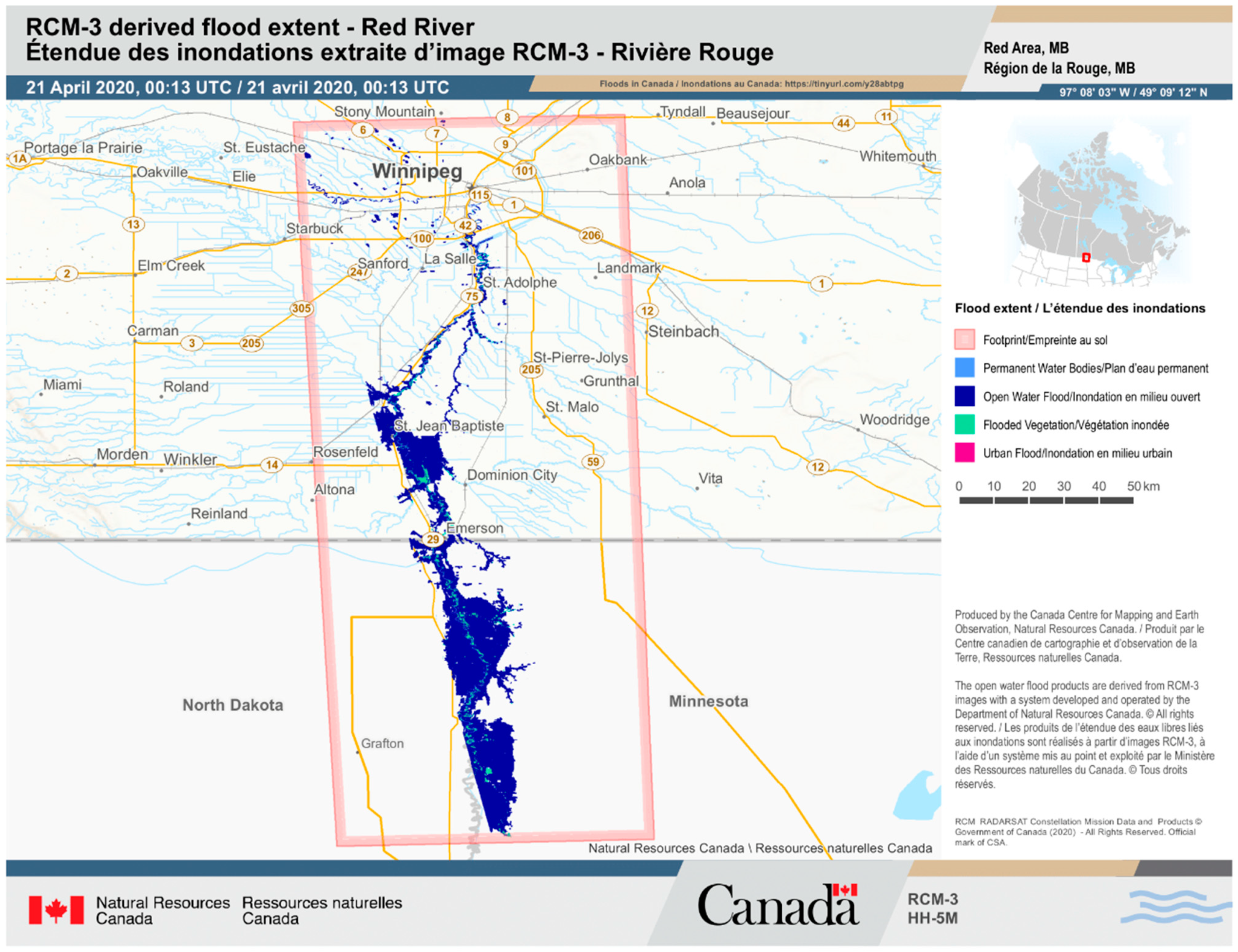
3.1. Flood Response

RCM data were used by the emergency geomatics service (EGS) for the first time to map flooding during the 2020 spring season on the Red River in southern Manitoba through Minnesota and parts of South Dakota. While research had been conducted on the use of CP to map open water and flooded vegetation in wetlands [14], 5 m spatial resolution dual-polarization RCM data consisting of HH and HV were ordered over the Red River instead of CP data for a number of reasons. First, while research was complete, operational flood tools were not yet fully developed to ingest and process CP, while EGS has expertise processing conventional dual-polarization data from years working with RADARSAT-2, requiring only minor modifications to existing flood tools to work seamlessly with RCM dual-polarization data. For the purpose of this application, 75 RCM frames acquired on 16 dates at 5 m spatial resolution were processed to generate and publish 20 flood maps spanning the duration of the flood event, from 14 April to 10 May 2020 (

Table 2. Summary of the RCM acquisitions.

Spacecraft Number	Date (UTC)	Time (hhmmss)	Imaging Beam	Polarization
RCM-1	14/04/2020	002049	HR5M	HH-HV
RCM-3	15/04/2020	123922	HR5M	HH-HV
RCM-3	16/04/2020	124741	HR5M	HH-HV
RCM-2	16/04/2020	000503	HR5M	HH-HV
RCM-2	17/04/2020	001301	HR5M	HH-HV
RCM-1	19/04/2020	123923	HR5M	HH-HV
RCM-1	19/04/2020	123859	HR5M	HH-HV
RCM-3	20/04/2020	000514	HR5M	HH-HV
RCM-3	21/04/2020	001312	HR5M	HH-HV
RCM-3	22/04/2020	002112	HR5M	HH-HV
RCM-3	23/04/2020	002911	HR5M	HH-HV
RCM-2	23/04/2020	123927	HR5M	HH-HV
RCM-2	23/04/2020	123936	HR5M	HH-HV
RCM-1	24/04/2020	000523	HR5M	HH-HV
RCM-1	27/04/2020	002849	HR5M	HH-HV
RCM-2	30/04/2020	002100	HR5M	HH-HV
RCM-2	05/05/2020	123911	HR5M	HH-HV
RCM-1	06/05/2020	000452	HR5M	HH-HV
RCM-3	09/05/2020	123922	HR5M	HH-HV
RCM-2	10/05/2020	000504	HR5M	HH-HV

). Furthermore, one RADARSAT-2 image was also processed to generate and publish a flood map over the case study area. The RADARSAT-2 image was a fine-quad 6.25 m spatial resolution image, acquired 12 h from an RCM image on the same date of 21 April, with incidence angles between 30.55° and 33.67°, compared to 33.63° and 35.93° incidence angles for the coincident RCM image.

EGS flood mapping methods, first used to map the major spring 2017 flooding event in Eastern Canada [16], were used during the 2020 Red River flood event. EGS flood mapping methods rely on a fully automated workflow that employs machine learning trained using scene-specific signatures representing multiple land and open water classes present in the scene, followed by region growing to map flooded vegetation and manual quality control editing. RCM data are first calibrated to sigma-naught, median filtered, orthorectified, and linearly scaled to 16-bit from a defined range (HH: 0 to 1, HV and VH: 0 to 0.15 and VV: 0 to 0.5) to 0–65,535 based on polarization to reduce file size. To map open water, dual-polarization signatures are sampled by overlaying the RCM image on an inundation frequency product generated from historical Landsat data [17] that depicts permanent land, represented by 0% frequency where water has never been observed, to 100% frequency representing permanent open water. Areas greater than 0% but less than 100% frequency are not sampled, since they represent ephemeral water where flooding might or might not be present on a given date. Once sampled, land and water signatures are used to train a random forest (RF) machine learning classifier to map the entire scene. Machine learning is used because it is a non-parametric classifier that makes no assumptions about the distribution of training data signatures. It is also able to learn from a large number of training data samples, eliminating the need to sub-sample a scene and ensuring that all classes and surface conditions are adequately represented in the training data. Further, as was demonstrated in [16], machine learning is generally robust to errors in training data [18,19]. Through simulation by introducing error into training data, [16] showed that the RF classification algorithm exhibits only a small performance penalty with up to approximately 30% error in training data in a binary land-versus-water classification. Therefore, any rare events that exceed historical flood extents present in the inundation frequency product by less than 30% will be mapped with similar quality. Lastly, machine learning is relatively time-efficient, enabling EGS to map and disseminate flood products within the required 4 h time period from data reception.

In addition to fully automated machine learning, manual dark-object thresholding of the HV channel was conducted on some scenes [20] where the automated results were determined to be suboptimal. As with other radar image data such as RADARSAT-2, this can occur when permanent water represents a small percentage of the overall image area, sometimes in combination with a dark return from snow or wet soil on land or specular reflection off of open water. Manual thresholding is sometimes performed in these cases where machine-learning fails, as it enables the analyst to control errors in the amount and configuration of the mapped flood water that can be added to or removed in subsequent steps.

Flooded vegetation is mapped next, if present as determined by the image analyst, which is the case along the Red River in 2020. Double-bounce off flooded vegetation causes a high-intensity return to the sensor, producing a bright signal in radar imagery, particularly in like-polarization channels [21]. The flooded vegetation algorithm region grows into these bright areas adjacent to open water, mapped previously using a high intensity threshold value in HH. This value lies somewhere between 10,000 and 12,000 DN in scaled 16-bit units, and is determined by examining the image in bright, double-bounce areas known to contain flooded vegetation based on cover type and elevation. The algorithm applies the threshold value to the entire image and selects objects adjacent to a mapped open water body that are brighter than this value. Open water and flooded vegetation maps are combined, and morphological operators, including sieving and infilling, are applied to remove small, false-positive water bodies and infill the interior of water bodies that were initially missed. This step is followed by manual editing, mainly to remove commission errors based on the analyst’s knowledge of the area, previous flood maps, and any additional information submitted in near real time from EGS’s Citizen Geographic Information (CGI) mobile application [16].

Rapidly changing flood extents and lack of available coincident ground-truth data make it difficult to quantitatively assess the accuracy of RCM flood maps; however, validation of the method applied to optical data for surface water extraction, prior knowledge of flooding in the region, visual image interpretation, and user feedback all confirm high flood mapping quality. Surface water maps generated from Landsat imagery using the EGS flood mapping methodology were validated against 30 m water fractions scaled from 1 m water masks and determined to be over 97% accurate in [22], which is nearly identical to the 96.9% overall accuracy obtained using manual thresholding of Landsat 5′s SWIR channel in [23]. In [16], we reported a 97.6% overall agreement and a kappa of 0.865 between 11 coincident Landsat and RADARSAT flood maps, including flooded vegetation, which suggests that the method applied to optical and radar imagery produces nearly identical maps, and therefore accuracy.

A user survey is distributed post flood season to Canadian federal and provincial stakeholders who use maps for a range of purposes, from near-real-time situational awareness for decision making, to distribution of financial aid during a flood crisis. Of the limited sample of 11 respondents in 2020, all rated EGS product accuracy as either good or excellent. For comparison, a user survey in 2019 had 26 respondents from activations in Manitoba, New Brunswick, southern Ontario, and Quebec. In total, 55 flood products were delivered this season, most of which were generated from RADARSAT-2 imagery. Of the 26 respondents, 23 rated EGS flood products as either having good or excellent accuracy, while 3 stated that accuracy was fair. Consecutive RCM and RADARSAT-2 products generated from data acquired 12 h apart on 21 April 2020 over the Red River show an overall agreement of 97.5% in the overlap region, which is substantial based on a kappa statistic of 0.76, and suggests good flood map continuity between the two satellite missions, despite changing floodwater extents in the 12 h period between acquisitions. Figure 1 presents an example of the obtained flood mapping using RCM on 21 April 2020.

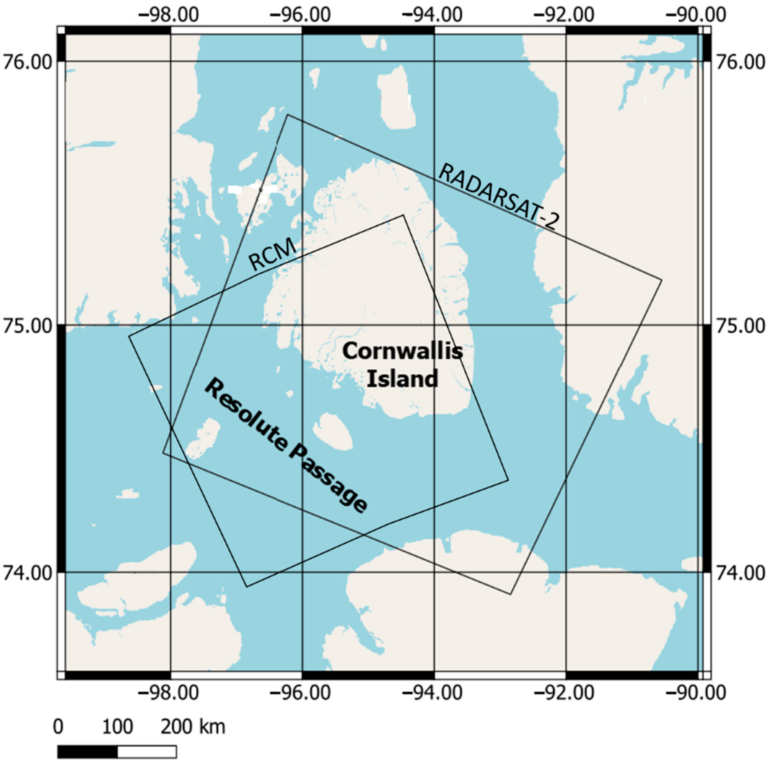
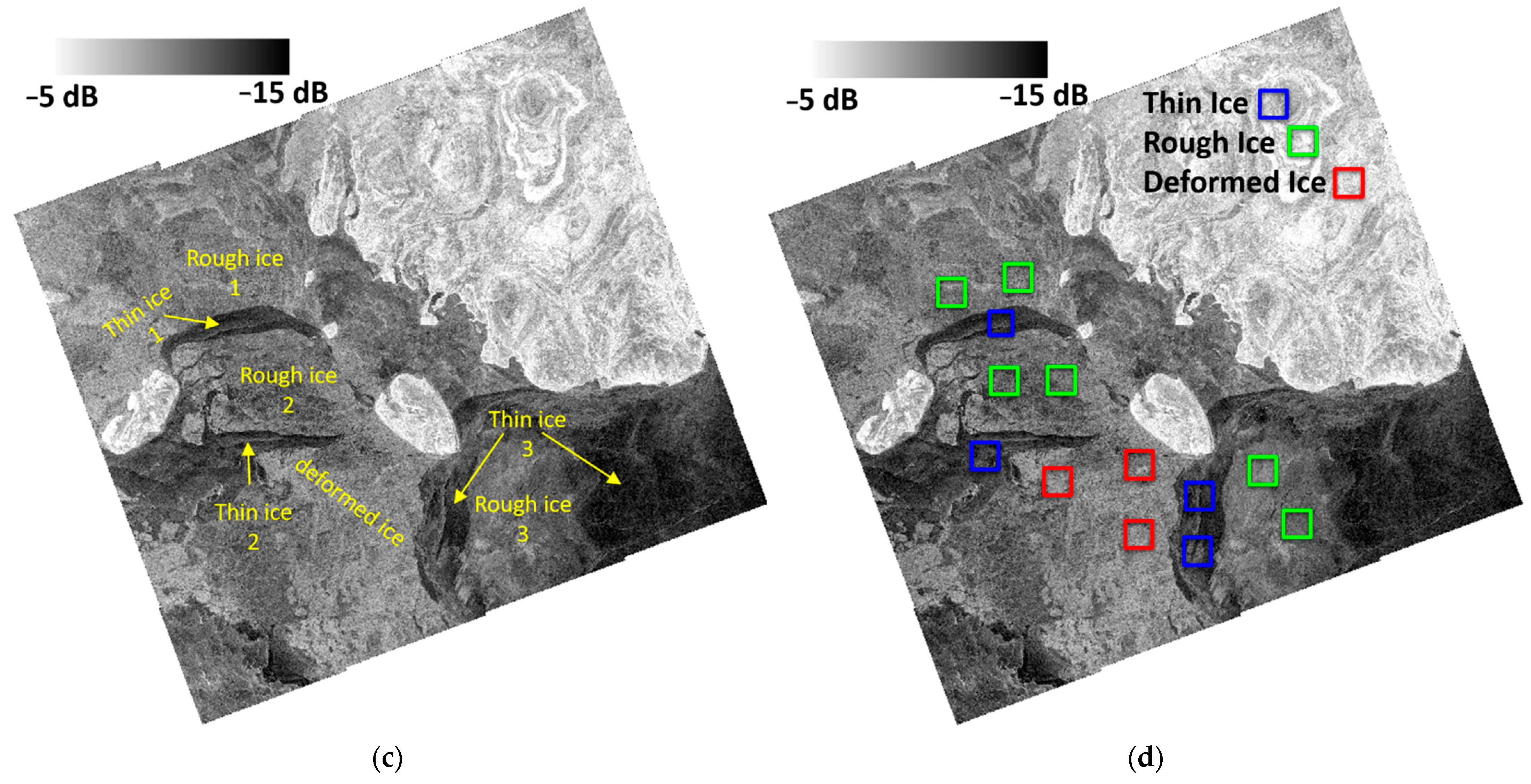
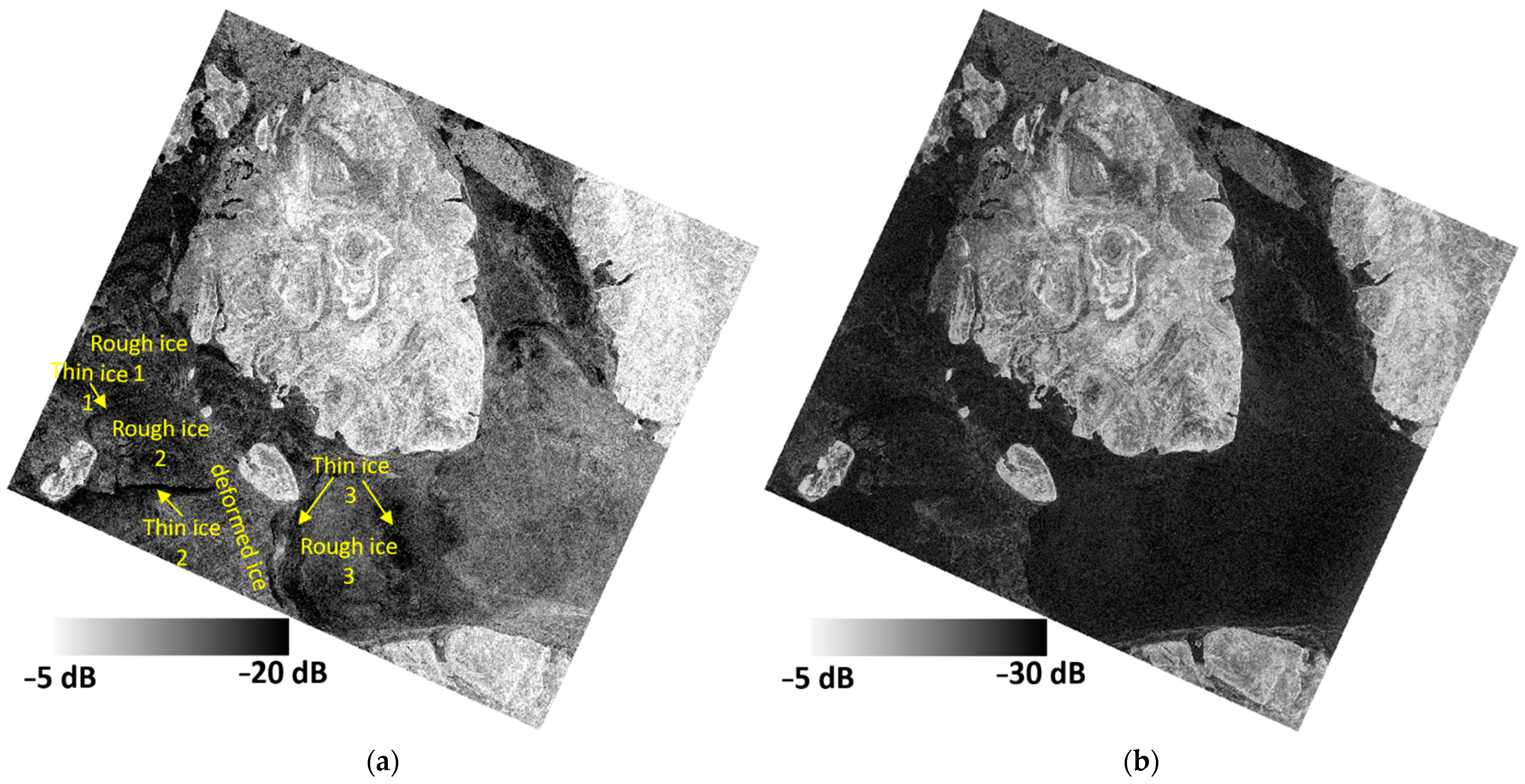
3.2. Sea Ice Analysis

Marine surveillance applications are one of the core RCM applications. Such applications include sea ice monitoring, which is one of the top priorities for Canada. This application has been highlighted because of the impact of climate change, which causes a decrease in ice thickness and extent in the Arctic. Continuation of this trend will facilitate new navigation opportunities via the Canadian Arctic Archipelago. The RCM is expected to fulfill the need for operational monitoring of sea ice by the CIS. The CIS is among the largest users of SAR imagery in the Canadian federal government [4]. Operational analysis of sea ice by the CIS pursues visual interpretation of SAR imagery in linear polarization, supported by ancillary information from several sources to map ice information in the form of daily ice charts. These charts compile information on ice types and open water, ice concentration, and surface topography features. For operational sea ice monitoring, CP SAR imagery is an attractive polarization option, given its similar spatial coverage to linear polarization, yet with increased radar target information [5,7].

In Figure 2, coincident RADARSAT-2 linear polarizations (HH and HV) and RCM compact polarization (RH and RV) images were acquired over the Resolute Passage, Canadian Central Arctic. The RADARSAT-2 SAR image from ScanSAR mode was acquired on 19 March 2020 while the RCM CP image from the ScanSAR medium resolution 30 m (SC30M) mode was acquired on 29 March 2020. A summary of the characteristics of the acquired imagery is shown in

Table 3. Metadata of the RADARSAT-2 and RCM Acquisitions.

	RADARSAT-2	RCM
Product	ScanSAR Georeferenced Fine Resolution (SGF)	SC30M Ground Range Detected (GRD)
Acquisition Date	19 March 2020	29 March 2020
Orbit Direction	Descending	Ascending
Polarization	HH, HV	RH, RV
Number of Looks	1 × 4	2 × 2
Incidence Angle	Near range = 19.5°, Far range = 31.2°	Near range = 17.2°, Far range = 28.9°
Spatial Resolution	30 m	30 m

. The acquired SAR images have similar spatial resolution and number of looks. Furthermore, the difference between the radar incidence angles at the center of the two images (2.3°) is negligible. Weather information available from the resolute weather station located in Cornwallis Island (Figure 2) showed that the daily average temperature during the month of March 2020 was always <−20 °C. During this period, the ice concentration reaches its peak value and the ice cover usually shows stable conditions that do not affect the observed backscatter from radar sensors.

Figure 3 shows the calibrated sigma naught backscattering images from both satellite missions. The combined knowledge of an ice expert and a CIS ice chart revealed the major ice types in the overlap area between the RADARSAT-2 and RCM images. As shown in Figure 3, the area consisted of different types of fast FYI, such as smooth thin ice, rough ice, and deformed ice. In comparison to HH (Figure 3a) and HV (Figure 3b), sea ice types appear to reveal higher contrast in RH (Figure 3c) and RV (Figure 3d). For example, the difference between thin and rough FYI is visually more pronounced in RH and RV compared to HH and HV (Figure 3). Analytically, the contrast between thin ice at locations 1 and 2 and the surrounding rough ice at locations 1 and 2 is enhanced in RH and RV. This contrast is reduced in HH and HV. This is also the case at location 3 of thin ice and location 3 of rough ice (Figure 3). Similarly, the contrast between deformed ice and the surrounding thin ice at locations 2 and 3 appears higher in RH and RV when compared to HH and HV. These findings could be linked to the contribution of both linear cross- and co-polarization in RH ($=\frac{1}{\sqrt{2}}(\mathrm{HH}-i\mathrm{HV})$) and RV ($=\frac{1}{\sqrt{2}}(\mathrm{VH}-i\mathrm{VV})$). The contrast between rough and deformed ice is visually less pronounced in both linear (RADARSAT-2) and circular (RCM) polarization when compared to the contrast between thin and rough as well as deformed ice (Figure 3).

It is worth noting that, unlike HH and HV, RH and RV in this specific case study appear to provide similar information content, with minor differences (Figure 3c,d). Although multiyear ice is not part of the ice cover composition, Figure 3 indicates that the CP SAR option produces visually appealing images, which holds a promise to improve the identification of ice types through the visual interpretation of CP SAR imagery.

We supported our visual analysis of the sea ice types in Figure 3 with the calculation of statistics of the different ice types in both RCM and RADARSAT-2 images.

Table 4. Mean and Standard Deviation of Sea Ice Types in RCM and RADARSAT-2 Images.

	RH (dB)			RV (dB)
	Thin Ice	Rough Ice	Deformed Ice	Thin Ice	Rough Ice	Deformed Ice
Mean	−9.71	−7.75	−6.37	−9.83	−7.76	−6.43
Stdev	1.19	1.16	1.25	1.10	1.17	1.27
	HH (dB)			HV (dB)
	Thin Ice	Rough Ice	Deformed Ice	Thin Ice	Rough Ice	Deformed Ice
Mean	−16.55	−16.46	−14.51	−26.83	−26.27	−24.91
Stdev	2.17	2.13	2.19	1.56	1.65	2.13

presents the mean and the standard deviation of thin, rough, and deformed ice, calculated from selected samples of ice types presented in Figure 3d. We note from Table 4 that the mean backscattering of the three ice types is quite close, with just small differences between RH and RV. Thin ice has an absolute difference between RH and RV equal to 0.12 dB. For rough and deformed ice types, the absolute difference between the mean backscattering in RH and RV is 0.01 and 0.06 dB, respectively. This confirms our previous visual analysis, which revealed similar information content of RH and RV for the selected case study. Only one combination (RH or RV) would be enough in this case. However, as expected, this is not the case for HH and HV. Herein, the absolute difference between HH and HV is 10.28 dB for thin ice, while for rough and deformed ice, the absolute difference is 9.81 and 10.40 dB, respectively. We note in Table 4 that RH backscattering is slightly higher than RV backscattering for all ice types. In the case of linear polarization, the co-polarization HH is consistently higher than the cross-polarization HV for all three ice types.

Table 5. Contrast of Sea Ice Types in RCM and RADARSAT-2 Images Expressed in Absolute Mean Backscattering Difference.

RH (dB)			RV (dB)
Thin Ice—Rough Ice	Thin Ice—Deformed Ice	Rough Ice—Deformed Ice	Thin Ice—Rough Ice	Thin Ice—Deformed Ice	Rough Ice—Deformed Ice
1.96	3.34	1.38	2.07	3.40	1.33
HH (dB)			HV (dB)
Thin Ice—Rough Ice	Thin Ice—Deformed Ice	Rough Ice—Deformed Ice	Thin Ice—Rough Ice	Thin Ice—Deformed Ice	Rough Ice—Deformed Ice
0.09	2.04	1.95	0.56	1.92	1.36

presents the contrast between the three ice types in the RCM and RADARSAT-2 imagery (Figure 3) expressed in terms of the difference in radar backscattering (Table 4) of the three ice types for different polarizations. As shown in Table 5, the absolute difference between thin and rough ice in RH and RV is 1.96 and 2.07 dB, respectively. This difference drops to 0.09 and 0.56 dB for HH and HV, respectively. For thin and deformed ice, the absolute difference in RH and RV is 3.34 and 3.40 dB, respectively. HH and HV reveal an absolute difference of 2.04 and 1.92 dB between thin and deformed ice, respectively. Interestingly, the contrast between rough and deformed ice appears to be slightly higher in HH and HV compared to RH and RV. This is because the absolute difference between these two ice types in HH and HV is 1.95 and 1.36 dB, while in RH and RV this difference slightly drops to 1.38 and 1.33 dB, respectively.

Table 5 shows that thin and deformed ice are the two ice types exhibiting the highest contrast in both RH and RV. This is also the case in HH and HV polarization. The lowest ice contrast in RH and RV is found between rough and deformed ice. Remarkably, this is not the case in HH and HV polarization, since the lowest contrast is shown between thin and rough ice. This could be an indication of the role of radar polarization (linear versus circular) in the discrimination between sea ice types.

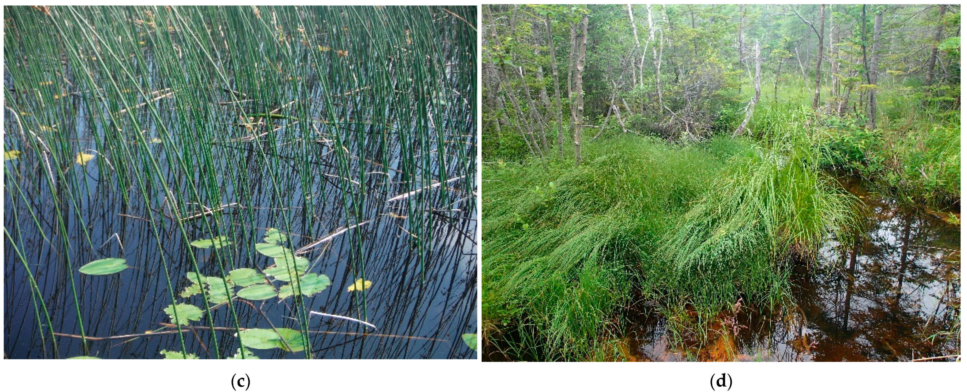
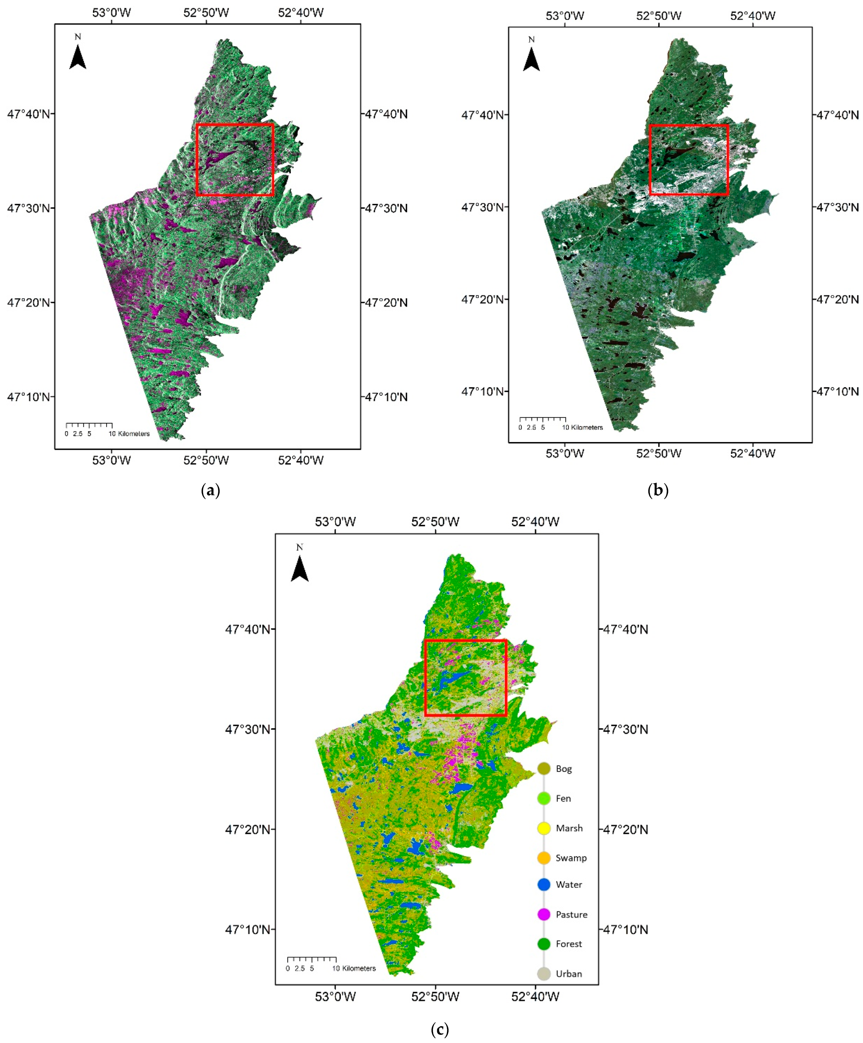
3.3. Wetland Monitoring

Although the capability of simulated RCM data has been previously investigated in several research studies for wetland mapping [12,13,24,25], the performance of real RCM data for this important natural resources is still lacking. This is of particular concern, as ecosystem monitoring in general, and wetland mapping in particular, is one of the RCM core applications. The province of Newfoundland and Labrador is a home to a great flora and fauna. Extensive research has been carried out for wetland mapping using various satellite imagery, including RADARSAT-2 [26] and simulated CP data [24], in this area. Figure 4 show the location of the study area for wetland classification in this study.

A wide variety of wetland classes categorized by the Canadian wetland classification system (CWCS), namely bog, fen, swamp, and marsh are available in the study area. This is an ideal case to investigate the capability of RCM data in combination with Sentinel-2 for wetland classification. For each class, reference polygons were sorted by size and alternatingly assigned to training and validation groups. This alternative assignment ensures that both the training and validation groups have comparable pixel counts for each class (i.e., 50% for training and 50% for validation). A description of the ground truth data used in this study for wetland classification can be found in [26]. Figure 5 demonstrates ground photo examples of these wetland classes.

The analysis over our wetland pilot site (Figure 4) was performed using RCM SC30M dual-polarized VV-VH data acquired on 25 July 2021. Given the insufficient polarimetric information within dual-polarized data for discriminating spectrally similar wetland classes [27], Sentinel-2 data was also acquired over the study area to aid in discriminating wetland classes. This imagery was acquired on 15 July 2021, relatively within a same time frame as of the RCM VV-VH data. SAR backscattering coefficient features and the ratio feature were extracted from SAR data. Five spectral bands—red, blue, green, near-infrared (NIR), and normalized difference vegetation index (NDVI) bands were also used as optical imagery features.

An object-based RF classification was performed using multi-source satellite imagery. In particular, multi-resolution segmentation was applied for object-based image analysis with the optimum parameters adopted from our previous research within the same study area [28]. The RF classification was performed with 500 for the number of trees (Ntree parameter) and the square root of the total number of features for the number of variables available for splitting at each tree node (Mtry parameter). It should be noted that Sentinel-2 and RCM data used in this study for wetland classification collect information about the bio-chemical and physical characteristics of wetland vegetation, respectively. Thus, the inclusion of both types of observations enhances the discrimination of backscattering/spectrally similar wetland classes. Figure 6 demonstrates the classification results from inclusion of RCM and Sentinel-2 imagery.

As demonstrated in Figure 6, this classification map distinguishes five wetland classes, namely bog, fen, marsh, swamp, and water, as well as three non-wetland classes, namely pasture, forest, and urban, within the study area. This map shows a clear separation of wetland classes, with sufficient details when it is compared with optical imagery. To better appreciate the classification details, Figure 7 illustrates a selected zoom-in area from the classification map (Figure 7c) along with RCM (Figure 7a) and Sentinel-2 (Figure 7b) imagery.

A comparison between Figure 7b,c illustrates an accurate separation of wetland and non-wetland classes. For example, all small water bodies and spectrally similar wetland classes (for example, bog and fen), which even represent no clear-cut border in the field, are well distinguished. The dominance of urban land cover in the zoomed area is also well represented. We supported our analysis of the classification results by the calculation of the classification confusion matrix, which we present in

Table 6. Classification confusion matrix of integrating Sentinel-2 and RCM data. An overall accuracy of 91.1% and kappa coefficient of 0.87 were obtained. UA refers to user’s accuracy, while PA refers to producer’s accuracy.

	Bog	Fen	Marsh	Swamp	Forest	Urban	Pasture	Water	UA (%)
Bog	15,917	5811	213	19	974	3	31	0	69.30
Fen	3271	18,191	27	1005	27	8	54	0	80.55
Marsh	134	101	7599	211	94	14	112	393	87.77
Swamp	125	66	118	4987	779	6	0	0	82.01
Forest	212	381	1301	73	8644	0	0	0	81.46
Urban	0	17	0	0	27	10,309	0	0	99.58
Pasture	0	0	0	0	0	0	5461	0	100.00
Water	0	0	0	0	0	0	0	88,966	100.00
PA (%)	80.97	74.50	82.08	79.22	81.97	99.70	96.52	99.56

.

As seen in Table 6, the urban, pasture, and water classes obtained producer’s (PA) and user’s accuracies (UA) of more than 95%, which represented the smallest omission and commission errors. Among wetland classes, bog and marsh had PAs better than 80%, with the marsh presenting the highest PA of 82.08%. However, for the fen and swamp, the PA was 74.50% and 79.22%, respectively. As such, fen had the highest omission error among all wetland classes. On the other hand, bog had the lowest UA of up to 69.30% and, as results, the highest commission error among all wetland classes. This was due to a large portion of the bog class being misclassified as fen class. Other wetland classes achieved UAs better than 80%, with the marsh exhibiting the highest UA, which reached 87.77%.

Notably, an overall accuracy of 91.10% and kappa coefficient of 0.87 are obtained for this object-based image analysis. This demonstrates promising results from dual-polarized VV-VH data when combined with other type of EO data for mapping wetland complexes.

4. Discussion

The RCM, with its advanced SAR technology (for example, CP architecture, the various imaging beam modes, the rapid revisit time, etc.) presents unique opportunities for Earth observation applications. It offers improved capabilities, which are expected to advance the operational SAR applications within not only Canada, but also globally. Furthermore, new emerging applications are anticipated, given the rapid revisit of the satellites and the adoption of CP with its wide swath in operational mode. This is supported by the availability of the CP option in all RCM imaging beam modes, except for the quad-polarization mode.

Initial results for a number of environmental applications showed promising performance using linear or compact polarization options. Disaster management, including among others, flood mapping, is one of the core RCM applications. The high level of agreement between the flood mapping results using RCM and RADARSAT-2 indicates a smooth transition of the operational flood mapping tools of EGS, but for linear polarization. However, the RCM flood mapping capabilities using real RCM CP data are yet to be investigated. Such investigation might require the modification of EGS operational flood mapping tools to adopt this new polarization.

Maritime surveillance applications, such as sea ice mapping, are also among the core applications of RCM. Sea ice mapping is the first operational SAR application within the Government of Canada since the time of RADARSAT-1, and has high potential for application of RCM data. It is expected the CP option to replace linear polarization in the process of ice chart generation at CIS. The visually enhanced discrimination capabilities between sea ice types compared to conventional linear polarization, shown in our initial analysis, could be a motivation for CIS towards the adoption of the CP option for the visual analysis of SAR imagery for sea ice monitoring. Enhanced ice information by RCM leads to safer marine navigation and commercial maritime transportation.

Another core application of RCM is ecosystem monitoring, which includes wetland classification. Given that wetlands are complex ecosystems with various types, detailed information about their spatial distributions and classes would require advanced remote sensing tools and data. The capabilities of RCM CP SAR data for wetland monitoring are yet to be investigated. However, first assessment of RCM linear dual-polarized imagery indicated a promising potential for the discrimination of wetland classes when fused with optical remote sensing imagery. The optical remote sensing support comes to complement the partial radar target information in RCM linear dual-polarized SAR imagery. This might not be the case for CP SAR imagery, since studies using simulated RCM CP SAR data indicate that the enhanced radar target information provided by this polarization option is efficient for monitoring complex dynamic ecosystems such as wetlands. This claim remains to be confirmed using real CP SAR imagery from RCM.

5. Conclusions

The purpose of this study was to report on initial results of RCM for selected SAR applications. The RCM was designed to address three core applications—disaster management, maritime surveillance, and ecosystem monitoring. Herein, we selected one case study application from each of the three themes to demonstrate an overview of the potential RCM performance for priority applications of interest for Canada.

Results indicated that operational flood tools designed for dual-polarized RADARSAT-2 data can be adopted for the case of RCM without major modifications. This indicates a smooth transmission from RADARSAT-2 to RCM within the operational flood mapping system at the EGS. This might not be the case once EGS adopts the CP SAR imagery option instead of the conventional linear dual-polarized SAR imagery. In this case, the EGS operational flood tools might need more than just a minor modification for optimized use of the enhanced radar target information provided by the CP SAR configuration.

Visual analysis of RCM CP SAR imagery over different sea ice types in dry ice winter conditions indicated improved contrast between thin ice and both rough and deformed ice when compared to coincident conventional linear dual-polarized SAR imagery from RADARSAT-2. These findings were confirmed statistically by calculating the absolute difference between the mean sea ice backscattering in linear and circular polarization. Statistical analysis indicated slightly higher contrast between rough and deformed ice in linear polarization. Further assessment of the performance of the RCM CP SAR configuration for sea ice monitoring and mapping is still necessary under various environmental conditions and radar incidence angles.

In the context of wetland monitoring, initial results reveal promising potential of RCM SAR data with partial polarimetric information for wetland classification. However, complementary remote sensing information, such as optical imagery, might be necessary for high classification accuracy. This could not be the case for wetland classification using RCM CP SAR imagery, given the increased radar target information.

Future work should focus on the evaluation of RCM for flood mapping, sea ice monitoring, and wetland classification in dedicated studies using data from different RCM imaging modes and under various environmental conditions.

References

1. Séguin, G.; Ahmed, S. RADARSAT constellation, project objectives and status. In Proceedings of the 2009 IEEE International Geoscience and Remote Sensing Symposium, Cape Town, South Africa, 12–17 July 2009; pp. 894–897. [Google Scholar]
2. Dabboor, M.; Iris, S.; Singhroy, V. The RADARSAT Constellation Mission in Support of Environmental Applications. Proceedings 2018, 2, 323. [Google Scholar] [CrossRef] [Green Version]
3. Raney, R.K. Hybrid-polarity SAR architecture. IEEE Trans. Geosci. Remote Sens. 2007, 45, 3397–3404. [Google Scholar] [CrossRef] [Green Version]
4. Charbonneau, F.; Brian, B.; Raney, K.; McNairn, H.; Liu, C.; Vachon, P.; Shang, J.; De Abreu, R.; Champagne, C.; Merzouki, A.; et al. Compact polarimetry overview and applications assessment. Can. J. Remote Sens. 2010, 36, S298–S315. [Google Scholar] [CrossRef]
5. Dabboor, M.; Geldsetzer, T. Towards sea ice classification using simulated RADARSAT constellation mission compact polarimetric SAR imagery. Remote Sens. Environ. 2014, 140, 189–195. [Google Scholar] [CrossRef]
6. Geldsetzer, T.; Arkett, M.; Zagon, T.; Charbonneau, F.; Yackel, J.; Scharien, R. All-season compact-polarimetry C-band SAR observations of sea ice. Can. J. Remote Sens. 2015, 41, 485–504. [Google Scholar] [CrossRef]
7. Dabboor, M.; Montpetit, B.; Howell, S. Assessment of the high resolution SAR mode of the RADARSAT constellation mission for first year ice and multiyear ice characterization. Remote Sens. 2018, 10, 594. [Google Scholar] [CrossRef] [Green Version]
8. Denbina, M.; Collins, M.J.; Atteia, G. On the detection and discrimination of ships and icebergs using simulated dual-polarized RADARSAT constellation data. Can. J. Remote Sens. 2015, 41, 363–379. [Google Scholar] [CrossRef]
9. Geldsetzer, T.; Charbonneau, F.; Arkett, M.; Zagon, T. Ocean wind study using simulated RCM compact-polarimetry SAR. Can. J. Remote Sens. 2015, 41, 418–430. [Google Scholar] [CrossRef]
10. Geldsetzer, T.; Khurshid, S.K.; Warner, K.; Botelho, F.; Flett, D. Wind speed retrieval from simulated RADARSAT constellation mission compact polarimetry SAR data for marine Application. Remote Sens. 2019, 11, 1682. [Google Scholar] [CrossRef] [Green Version]
11. Dabboor, M.; Singha, S.; Montpetit, B.; Deschamps, B.; Flett, D. Pre-launch assessment of RADARSAT constellation mission medium resolution modes for sea oil slicks and lookalike discrimination. Can. J. Remote Sens. 2019, 45, 530–549. [Google Scholar] [CrossRef] [Green Version]
12. Dabboor, M.; White, L.; Brisco, B.; Charbonneau, F. Change detection with compact polarimetric SAR for monitoring wetlands. Can. J. Remote Sens. 2015, 41, 408–417. [Google Scholar] [CrossRef]
13. Dabboor, M.; Banks, S.; White, L.; Brisco, B.; Behnamian, A.; Chen, Z.; Murnaghan, K. Comparison of compact and fully polarimetric SAR for multitemporal wetland monitoring. IEEE J. Sel. Top. Appl. Earth Obs. Remote Sens. 2017, 12, 1417–1430. [Google Scholar] [CrossRef]
14. Olthof, I.; Rainville, T. Evaluating simulated RADARSAT constellation mission (RCM) compact polarimetry for open-water and flooded-vegetation wetland mapping. Remote Sens. 2020, 12, 1476. [Google Scholar] [CrossRef]
15. Kroupnik, G.; De Lisle, D.; Côté, S.; Lapointe, M.; Casgrain, C.; Fortier, R. RADARSAT constellation mission overview and status. In Proceedings of the 2021 IEEE Radar Conference (RadarConf21), Atlanta, GA, USA, 7–14 May 2021; pp. 1–5. [Google Scholar]
16. Olthof, I.; Tolszczuk-Leclerc, S.; Lehrbass, B.; Shelat, Y.; Neufeld, V.; Decker, V. New Flood Mapping Methods Implemented during the 2017 Spring Flood Activation in Southern Quebec; Geomatics Canada: Chatham-Kent, ON, Canada, 2018. [Google Scholar]
17. Pekel, J.F.; Cottam, A.; Gorelick, N.; Belward, A. High-resolution mapping of global surface water and its long-term changes. Nature 2016, 540, 418–422. [Google Scholar] [CrossRef]
18. Ghosh, A.; Manwani, N.; Sastry, P.S. On the robustness of decision tree learning under label noise. In Advances in Knowledge Discovery and Data Mining; Kim, J., Shim, K., Cao, L., Lee, J.G., Lin, X., Moon, Y.S., Eds.; Springer: Berlin/Heidelberg, Germany, 2017; Volume 10234, pp. 685–697. [Google Scholar]
19. Frénay, B.; Verleysen, M. Classification in the presence of label noise: A survey. IEEE Trans. Neural Netw. Learn. Syst. 2014, 25, 845–869. [Google Scholar] [CrossRef] [PubMed]
20. Brisco, B.; Short, N.; Van der Sanden, J.; Landry, R.; Raymond, D. A semi-automated tool for surface water mapping with RADARSAT-1. Can. J. Remote Sens. 2009, 35, 336–344. [Google Scholar] [CrossRef]
21. Hess, L.L.; Melack, J.M.; Simonett, D.S. Radar detection of flood beneath the forest canopy: A review. Int. J. Remote Sens. 1990, 11, 1313–1325. [Google Scholar] [CrossRef]
22. Olthof, I. Mapping seasonal inundation frequency (1985–2016) along the St-John River, New Brunswick, Canada using the Landsat archive. Remote Sens. 2017, 9, 143. [Google Scholar] [CrossRef]
23. Frazier, P.S.; Page, K.J. Water body detection and delineation with Landsat TM data. Photogramm. Eng. Remote Sens. 2000, 66, 1461–1467. [Google Scholar]
24. Mohammadimanesh, F.; Salehi, B.; Mahdianpari, M.; Brisco, B.; Gill, E. Full and Simulated Compact Polarimetry SAR Responses to Canadian Wetlands: Separability Analysis and Classification. Remote Sens. 2019, 11, 516. [Google Scholar] [CrossRef] [Green Version]
25. Mahdianpari, M.; Salehi, B.; Mohammadimanesh, F.; Brisco, B. An Assessment of simulated compact polarimetric SAR data for wetland classification using random forest algorithm. Can. J. Remote Sens. 2017, 43, 468–484. [Google Scholar] [CrossRef]
26. Mahdianpari, M.; Salehi, B.; Mohammadimanesh, F.; Motagh, M. Random forest wetland classification using ALOS-2 L-Band, RADARSAT-2 C-Band, and TerraSAR-X imagery. ISPRS J. Photogramm. Remote Sens. 2017, 130, 13–31. [Google Scholar] [CrossRef]
27. Mahdianpari, M.; Mohammadimanesh, F.; McNairn, H.; Davidson, A.; Rezaee, M.; Salehi, B.; Homayouni, S. Mid-season crop classification using dual-, compact-, and full-polarization in preparation for the RADARSAT constellation mission (RCM). Remote Sens. 2019, 11, 1582. [Google Scholar] [CrossRef] [Green Version]
28. Mohammadimanesh, F.; Salehi, B.; Mahdianpari, M.; Brisco, B.; Motagh, M. Multi-temporal, multi-frequency, and multi-polarization coherence and SAR backscatter analysis of wetlands. ISPRS J. Photogramm. Remote Sens. 2018, 142, 78–93. [Google Scholar] [CrossRef]
Figure 1. Flood mapping of Red River, Manitoba, using RCM acquisition on 21 April 2020.
Remotesensing 14 00301 g001
Figure 2. RADARSAT-2 and RCM acquisitions over the Resolute Passage, Canadian Central Arctic.
Remotesensing 14 00301 g002
Figure 3. Backscattering coefficients of (a) RADARSAT-2 HH, (b) RADARSAT-2 HV, (c) RCM RH, and (d) RCM RV.
Remotesensing 14 00301 g003aRemotesensing 14 00301 g003b
Figure 4. The location of the study area with an overlay of RCM data.
Remotesensing 14 00301 g004
Figure 5. Ground reference photos showing wetland classes in the study area: (a) Bog; (b) fen; (c) marsh; and (d) swamp.
Remotesensing 14 00301 g005aRemotesensing 14 00301 g005b
Figure 6. (a) Color composites of RCM data (R: VV, G: VH, B: VH/VV) (b) True color composite of Sentinel-2 imagery, and (c) Classification map of the study area, discriminating eight land cover classes. Red frame indicates a selected zoom-in area in Figure 7.
Remotesensing 14 00301 g006
Figure 7. The selected zoom-in area (red frame in Figure 6) from (a) RCM (R: VV, G: VH, B: VH/VV), (b) Sentinel-2, and (c) classification map.
Remotesensing 14 00301 g007