Abstract
Satellite remote sensing provides useful gridded data for the conceptual modelling of hydrological processes such as precipitation–runoff relationship. Structurally flexible and computationally advanced AI-assisted data-driven (DD) models foster these applications. However, without linking concepts between variables from many grids, the DD models can be too large to be calibrated efficiently. Therefore, effectively formulized, collective input variables and robust verification of the calibrated models are desired to leverage satellite data for the strategic DD modelling of catchment runoff. This study formulates new satellite-based input variables, namely, catchment- and event-specific areal precipitation coverage ratios (CCOVs and ECOVs, respectively) from the Global Precipitation Mission (GPM) and evaluates their usefulness for monthly runoff modelling from five mountainous Karkheh sub-catchments of 5000–43,000 km2 size in west Iran. Accordingly, 12 different input combinations from GPM and MODIS products were introduced to a generalized deep learning scheme using artificial neural networks (ANNs). Using an adjusted five-fold cross-validation process, 420 different ANN configurations per fold choice and 10 different random initial parameterizations per configuration were tested. Runoff estimates from five hybrid models, each an average of six top-ranked ANNs based on six statistical criteria in calibration, indicated obvious improvements for all sub-catchments using the new variables. Particularly, ECOVs were most efficient for the most challenging sub-catchment, Kashkan, having the highest spacetime precipitation variability. However, better performance criteria were found for sub-catchments with lower precipitation variability. The modelling performance for Kashkan indicated a higher dependency on data partitioning, suggesting that long-term data representativity is important for modelling reliability.
1. Introduction
Managing surface water resources is challenged by prolonged droughts and intensified floods under a changing climate. Consequently, larger fluctuations of river runoff (i.e., water discharge arriving at a river point per time step) induce problems for water managers in the developing world [1,2], where natural hazards are causing poverty, hunger, migration, and casualties [3,4]. In this sense, reservoirs are valuable in alleviating this fluctuation by water storage during abundance for future shortages. However, the supply-oriented water management system is usually argued to be a fix that can backfire [5] due to the false interpretation of available water, deterioration of the ecosystem through a flooded upstream and dried out downstream, and upstream–downstream conflicts they may create. Regardless of the pros and cons of damming natural flows, the proper operation of existing river–reservoir systems is necessary. The inflow is usually a major determinant of the behaviour of a water supply system. Combined with the measured variables (e.g., withdrawals), inflow estimates can be used to calculate other water balance components for simulation problems [6]. For example, the estimated inflow, combined with the known storage capacity and rule curves of the reservoir, is used to calculate the water loss due to evaporation under different hydrological scenarios. This depends on the evaporation rate (e.g., from the pan equation) and water surface area from the water balance equation and volume–area relationships of the reservoir [7]. So, accurate runoff modelling is important for reliable water management and, thereby, developing proper decision-support systems for plausible future scenarios. Rainfall–runoff models are useful computer tools for inflow simulation primarily by relating precipitation and discharge (runoff) data in a catchment. Major reservoirs in the semi-arid climate are typically built downstream of large mountainous catchments suffering from insufficient spacetime observations of the underlying factors such as areal precipitation based on sparse observations [8,9,10,11].
Rainfall–runoff models range from black-box to physical-based models [12]. While the earlier relate certain input variables to outputs using identifiable patterns in the data alone through well-known mathematical formulas, the latter may require such large datasets and detailed knowledge of the physical processes that they are often of limited use [13]. Due to the advancements in computational methods, however, black-box models have rapidly progressed and been raised to an area referred to as data-driven (DD) modelling. Artificial Neural Networks (ANNs) are undoubtedly the most popular, successful type of Artificial Intelligence (AI)-assisted DD models introduced to hydrology [14,15,16,17,18,19,20,21]. Nonetheless, no physical insight in DD models is a fundamental shortcoming. Conceptual modelling is another type of modelling that rather faithfully explains hydrological processes through simplified conceptions [22,23,24]. The unit hydrograph (UH) notion based on the concept of proportionality and superposition of time-invariant responses of runoff to excess rainfall is a basic example. As discussed in [25], linear systems are an important part of applied hydrology since the introduction of the UH. However, the response to a precipitation event is not independent of the state of the catchment, including the initial soil moisture, vegetation status, and evaporation rate that are all highly time-dependent. Major deviations from linearity are attributed to the variation of evapotranspiration (ET) and the accumulation of the soil moisture deficit in dry periods [25]. Conceptual models can be either spatially lumped or spatially distributed. IHACRES, for example, is a widely used lumped model, e.g., [7,13,26,27,28,29]. It applies a non-linear loss function to estimate the catchment-scale excess rainfall and a linear UH module to convert the excess rainfall to runoff using a grid search parameterization in user-specified steps and ranges of some parameters. The TOPX model is a more sophisticated example that adopts a topography-based process and combines methods such as a linear reservoir, and the Muskingum equation to route the land, base, and channel flow components, while the calibration is based on trial-and-error [30]. In any case, semi-distributed conceptual models can reflect the spatial variation of input variables only by dividing a catchment into sub-catchments.
Satellite remote sensing (RS) of the land surface, vegetation, and atmosphere provides supplementary or alternative data for runoff simulations where in situ data are unsatisfactory. The grid format of the RS data has made these popular for distributed models such as SWAT [31,32]. However, closing the water budget of the spatially distributed physical models is a computationally expensive process. This usually limits the calibration to the use of a single land-use map, among other simplifications. Moreover, RS data are subject to different errors, e.g., due to their indirect estimation methods rather than direct measurements. Therefore, they need correction before use [33], based on some reference measurements such as those PRISM Climate Data provides for the US [34]. There are regional to global-scale bias-corrected RS data. However, the adjusted data may still be inaccurate, if not worsened [35] primarily because the scale and nature of gauge–satellite data may not be compatible. For example, a normal rain gauge measures the accumulation of precipitation at a local point over a period, while RS estimates the precipitation intensity over rather large grid sizes in discrete time. Therefore, bias-corrected data may carry a level of uncertainty that can accordingly result in a poor runoff simulation. Not to mention that remote, data-scarce catchments may have no way to ensure the bias correction. The calibration of ANN models is based on machine learning (more accurately, deep learning) algorithms that are well-known for the effective modelling of complex non-linear systems. Therefore, unadjusted input data for possible bias may not necessarily result in a biased output if we accept that bias is a pattern in the repeated errors and fixable by linear or non-linear methods. Many studies have recently focused on the use of AI-assisted DD models for improving RS inputs such as precipitation [36,37,38,39]. While bias in the input is still an important source of uncertainty in RS hydrology, another major concern regarding DD models that was not addressed well is how to implement the spatially distributed RS data effectively in black-box modelling approaches. The larger size of ANNs due to many input variables, e.g., equivalent to several tens of grids within a catchment for each involved element (e.g., precipitation, ET, etc.), is not a proper way to handle the calibration. Especially, when the length of data is short, the representation of all possible variations of catchment responses to different areal precipitation is not possible. Alternatively, data from the original grid sizes can be averaged over a few sub-catchments or be rescaled to larger grid sizes to reduce the size of the ANN. For shorter time scales (hourly to daily), the sub-catchments may be classified based on the lag time (elapsed time between the occurrence times of excess precipitation and runoff), while for monthly to seasonal scales, useful for strategic surface water management, the lag time may be negligible. At any rate, a degree of spatial variation may be lost due to employing larger sub-catchments.
In view of the above, this study introduces areal precipitation coverage ratios, derived from the original, smallest RS grids, as new input variables to the ANN to compensate for the lost variation due to the use of average precipitation over sub-catchments. Therefore, the main presumption of the study is whether, and how, the runoff variation can be explained by using the areal coverage ratios via DD modelling with the computational advantages discussed above. Furthermore, recently, attempts were undergone to use hybrid models in a hydrological simulation, mainly by combining outputs of several synergetic DD models [40,41]. Thus, we used simple but generalized hybrids of individual ANNs. A way to conceptualize DD models is achieved when pre-processed input variables are employed. Therefore, the added value of other RS data, including the vegetation index, and ET were investigated combined with and without the areal precipitation coverage ratios. Moreover, seasonality and the possible memory of the response (runoff) were considered by integrating outputs of seasonal runoff models and time-lagged input variables for 0–2 months. Finally, an adjusted cross-validation and verification process, as well as different configurations and random initial parameterizations of the ANN models were evaluated to avoid overfitting and ensure the generalization of the outputs.
2. Study Area and Data
2.1. Study Area
The Karkheh River Basin (KRB) in west and southwest Iran is among the three most hydrologically productive (i.e., producing high runoff amounts) basins of the country. With 3.5 million residents, it is a highly populated basin in Iran [42]. The KRB is a rather small section of the enormous, transboundary Tigris–Euphrates catchment. The case study covered the majority of the KRB upstream of the Karkheh Dam (Figure 1). Being in operation since 2002, the dam creates the largest artificial reservoir in Iran with a 5.6 BCM normal storage. The reservoir’s main purpose is agricultural development, hydropower generation, and flood control in Khuzestan. The operation of the reservoir has become a challenging task due to the unpredicted inflow variation under prolonged drought and unprecedented floods in recent decades. As shown in Figure 1a,b, the study area is dominated by a mountainous topography. This area is nearly 42,900 km2 and comprised of two major sub-catchments, known by their main rivers, i.e., Seymareh (I–III) and Kashkan (IV), and a smaller area (V) after the two upstream branches meet and create Karkheh River (Figure 1c). In this study, two upstream tributaries of Seymareh, i.e., Gamasiab (I) and Qarasu (II), with areas of 11,500 and 5500 km2 were segmented to have catchments of different sizes evaluated. The altitude of the KRB ranges from some five meters in the southwest, where the river eventually ends at the Hawizeh Marshes (or Hoor al-Azim) on the Iran–Iraq border, to above 3500 m in the upstream highlands of the Zagros Mountains.
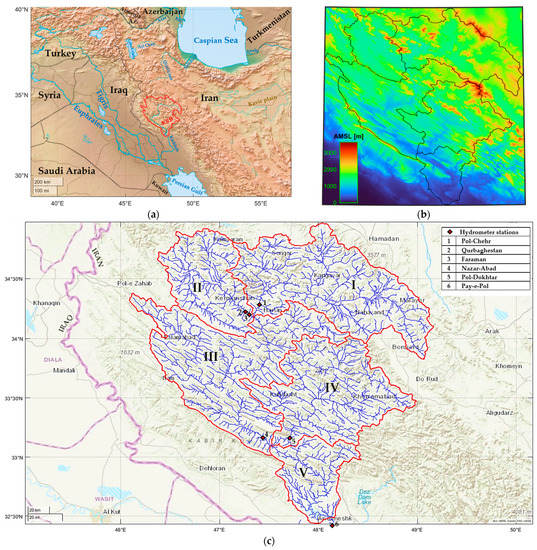
Figure 1.
Location of the KRB upstream of the Karkheh Dam in west Iran (a), and its elevation map (b) over sub-catchment areas (c) of Gamasiab (I), Qarasu (II), Seymareh (I–III), and Kashkan (IV). The entire study area of KRB covers all areas I–V.
2.2. Hydrological Data
The runoff data for the studied sub-catchments were obtained from the closest hydrometer station to their outlet point (Figure 1c) and possible differences between the outlet and the station were neglected as a usual practice in water resource planning of the catchment. Table 1 shows the mean, maximum, coefficient of variation (CV), skewness, and kurtosis of the average monthly discharge data for the water years in Iran between the 23rd of September in 1999 and the 22nd of September in 2017. The start year was chosen based on the availability of the satellite products (introduced in the next Sections), while the end year was imposed by the availability of data on the website of the Iran Water Resources Management Company, the official organization for the national reports of hydrological data. As clarified below, the final data length for the modelling purpose was 205 months from mid-2000 (limited by the satellite precipitation data) to September 2017 (limited by runoff data) after excluding the two first months due to time-lagged inputs. In general, the longer the data, the more reliable model one may expect. However, it is important to note that data efficacy is also a matter of context and purpose of use. For instance, Refs. [43,44] used data lengths of 110–221 months for monthly rainfall–runoff modelling using ANNs. As described later in more detail, the present study focused on evaluating the usefulness of new input variable combinations and employed an adjusted k-fold data partitioning and model development process that helps avoid overfitting and assures keeping data for the verification of the model regardless of the data length. It is also noted that the study relied on RS-based data except for the runoff data.

Table 1.
The drainage basin area and overview of monthly average runoff data in the different sub-catchments of the KRB for the period between September 1999 and September 2017.
Figure 2 shows monthly average runoff data based on all available historic data for the Pay-e-Pol station (1954–2017), the representative station of the KRB that receives runoff from the entire study area. According to the start of the first month in the water year in late September (first of month 7 in Solar Hijri calendar) in Iran, the maximum discharge usually occurred in months 6–8, March–May, which corresponded to the highest variability of runoff. In Figure 2, an extreme value in month three for the top percentile (95–100%) compared to the usually lower values was noted for November–December. This value corresponded to a severe flood event in late November 1994. Thus, it was outside the studied period for the modelling as described earlier (2000–2017). The observed variation for the 205 months of data used for the modelling is presented and discussed in the Results Section using time series hydrographs and quantile–quantile (q–q) plots.
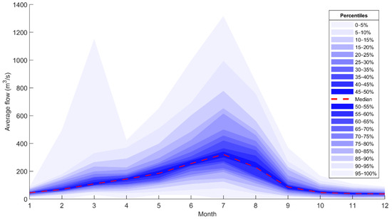
Figure 2.
Monthly average discharge variability at the Pay-e-Pol station downstream of Karkheh Dam for local water years between 1954 and 2017 (for months when Karkheh and Seymareh dams existed, data were estimated by observations at closest upstream stations).
2.3. GPM-IMERG Precipitation
As a successor to the Tropical Rainfall Measuring Mission (TRMM), the Global Precipitation Measurement (GPM) was launched by the mission of the GPM Core Observatory satellite that unifies estimates of an international constellation of satellites for an improved precipitation observation globally. Integrated Multi-SatellitE Retrievals for GPM (IMERG) combine intermittent observations from microwave sensors on the constellation into merged half-hourly 0.1 × 0.1 fields by a morphing process integrating geostationary infrared satellites [45,46]. The IMERG algorithm is now run for both TRMM and GPM eras (since 2000) [46,47]. The two near real-time runs of the IMERG, namely, Early and Late, result in two half-hourly datasets by about 4 h (shorter for the second halves of hours) and 14 h (12 h for recent data) after the observation time, respectively.
IMERG-Late uses data from more sources than IMERG-Early and, since it waits for the next overpass of satellites, employs both forward and backward propagation in the morphing process. The IMERG-Final product is bias corrected using monthly observations from rain gauges around the globe (by the GPCC: Global Precipitation Climatology Centre) and is available with a minimum latency of 3.5 months. Thus, it is not suitable for applications that require near real-time data. NASA comments that IMERG-Final and IMERG-Late products are similar (mainly over oceans, and, to a lesser extent, over land). Referring to the results of the previous study of IMERG products over Iran [35], IMERG-Late overperformed IMERG-Early and showed comparable results with IMERG-Final in the study area. Contrary to IMERG-Late, however, IMERG-Final significantly underestimated extreme precipitation, particularly in spring (March–May) concurring the highest runoff values in the study area. Moreover, as discussed in the introduction, data-scarce catchments may have no way to ensure the bias adjustment. Thus, both the case study situation and the general aim of the study to benefit data-scarce catchments advocated the use of IMERG-Late here. Consequently, this study used the daily PrecipitationCal product from Version 06 of IMERG-Late with available data since June 2000.
2.4. MODIS Products
The Moderate Resolution Imaging Spectroradiometer (MODIS), comprised of two passive satellites, Terra and Aqua, views the entire Earth (including clouds, aerosols, land, and water surfaces) every 1–2 days in 36 wavelength bands with resolutions 250, 500, and 1000 m for bands 1–2, 3–7, and 8–36, respectively. There are composite datasets introduced based on MODIS that combine other data sources with the RS data from Terra or Aqua. This study used both composite and band data as described below. MODIS data were generated in square tile units of 1200-by-1200 km (at the equator) in the HDF-EOS format. Thus, more than a tile may be needed to cover an area of interest on the ground.
It is worth mentioning that a concern using satellite imagery is the spatial resolution and revisit time. For instance, Landsat, in comparison to MODIS, provides a higher spatial resolution (30–100 vs. 250–1000 m), but a longer revisit time (16 days vs. daily). On the other hand, geostationary satellites meet the temporal resolution requirement of many applications but suffer from a too coarse spatial resolution. Two newer satellites, Sentinel 2A and 2B, that together present a more balanced spatiotemporal resolution in the clear sky (every 5–10 days and 10–60 m) have limited records compared to MODIS (since 2015 and 2017 vs. 2000).
2.4.1. MODIS-Terra Evapotranspiration Product
The version 6 MODIS terrestrial ecosystem evapotranspiration (ET) and potential ET (PET) data product (MOD16A2v006 [48]) are eight-day 500-m composite datasets based on the Penman–Monteith model. It includes inputs of daily meteorological reanalysis data along with other products such as the vegetation property, albedo, and land cover. The year-end gap-filled eight-day MOD16A2 Version 6 data product at a 500 m pixel size was used to calculate the monthly catchment-wide PET and ET in the study.
2.4.2. MODIS-Terra Vegetation Index Product and Band 7 Data
MOD13 Series [49] include MODIS vegetation index products at 16-day and monthly and multiple grid sizes equal to or smaller than 1 km. This study used the monthly standard Normalized Difference Vegetation Index (NDVI) data from the MOD13A3 Version 6 product at a 1 km resolution to calculate spatially averaged vegetation time series for the sub-catchments. MODIS has specific bands that are useful for estimating soil moisture. For example, Ref. [50] showed that a mid-IR band of MODIS, i.e., Band 7 (B7), with an original 500 m pixel size, has a good correlation with in situ soil-moisture observations. The B7 data coming with the NDVI data in the MOD13A3 Version 6 product were used here.
3. Methodology
The methodology of the study combined satellite-based data introduced above [32,35,45,46,48,49,50] to formulate new collective input variables for improved modelling of catchment runoff response to areal precipitation using Artificial Intelligence (AI)-assisted DD approaches. The ANNs [14,15,43] and a k-fold process [51,52,53] with the adjustment described in the following Sections were used as reference for the evaluation. Both statistical and visual comparisons (introduced below) between modelled and observed discharge were performed. A particular aim of the present study was to improve simulation of monthly runoff from the five sub-catchments of the KRB in a mountainous environment. Such a study area characteristic largely demands for improved hydrological modelling according to the literature [9,10,11]. The results of the study could increase added values of both satellite data and DD models for large-scale hydrological simulations and strategic surface water management at sparsely gauged locations. In conclusion, the novelty of the study lies in the new satellite-based input variable formulation for DD modelling of monthly runoff, and the hybrid scheme for generalization of the ANN model.
3.1. Modelling Architecture and Settings of ANN
Resembling human mind traits, i.e., learning for problem-solving, ANNs are a well-known type of AI models. ANNs are DD-machine learning systems that are widely used for non-linear function fitting problems in hydrology. The architecture of an ANN is based on a set of connected neurons spread over one or more hidden layers, for shallow to deep networks, between input and output layers [14,15,18]. The input and output variables are vectors of equal size for time series of involved variables (precipitation, ET, etc.) and runoff, respectively. The simplest ANN model can be thought of as a single neuron in a hidden layer. This neuron multiplies each input vector (, where is number of input variables) in the input layer with a scalar weight , and adds sums of weighted inputs with a scalar bias to allocate to the neuron, where and are typically random values between −1 and 1. Next, an activation (or transfer) function was applied to , i.e., , to produce first estimation of the output variable (i.e., runoff) in the range of, e.g., 0 to 1, −1 to 1, or beyond if a log-sigmoid, a hyperbolic tangent sigmoid, or a linear transfer function is employed, respectively. Since input variables and runoff are usually normalized over −1 and 1 before use in the ANNs, estimated outputs must be returned to the previous scale to give actual runoff estimates.
For larger ANNs, each neuron in each layer treats outputs of all neurons in the previous layer as inputs and so forth. This one-way non-recurrent data progress for model development is known as feedforward. Thus, the output layer of an ANN with one output variable (runoff) is always a single neuron that transfers the previous hidden layer’s outputs to estimates of the output variable. Consequently, estimates of the runoff vector from a three-layer ANN can be written as [54]:
where superscripts denote layer number, and and are and matrices of the input variables (involving features) and weights, respectively. Additionally, b is a scalar value representing bias, is estimated output vector of length, and is number of input–output data pairs, equivalent to the studied length of monthly runoff time series (i.e., 205). The transfer functions may differ from one layer to another. They control the non-linearity of the modelling, and, without them, ANNs are nothing but a group of linear functions of input variables [15]. Nevertheless, the functions should be differentiable with respect to parameters (i.e., and ) to be optimized using gradient- or Jacobian-based methods after some iterations. For the final output layer (here, ), the study used a linear function, i.e., , while, for the hidden layers (here, and ), the hyperbolic tangent sigmoid transfer function was adopted expressed as [54]:
Upon initialization with a random set of parameters ( and ), the ANN repeatedly adjusted them by determining direction and steps at each iteration to minimize the loss function as an equation of the model’s residual (i.e., difference between estimated and observed runoff) until a stopping rule was met, i.e., when the gradient was close to zero, the step size for parameterization was too small, or the number of iterations (epochs) exceeded a specified limit. This study applied a backpropagation learning algorithm based on the chain rule of the calculus as described in [54] and the mean squared error performance criteria for the loss function [54,55]:
where, and are time series of observed and simulated runoff ( = 1, …, ).
A consequence of setting a too loose stop rule for ANN is overfitting during learning. Keeping a portion of the available data for validation is, therefore, necessary. An efficient, in-process way to skip overfitting is to set an early stopping rule for the learning process by checking model performance in each iteration for the validation portion of the data not used for parameterization. Thus, continuous reduction in the model performance for the kept-out, validation data by iteration for certain times (i.e., maximum number of validation fails) can be considered a signal of overfitting that stops the parameterization process. The modelling parameters were stored for each iteration, and the final model was fixed with parameterization based on the minimum value of loss function for validation.
Prior knowledge of architecture and settings for an ANN that best suits a hydrological problem is difficult to incorporate [14]. Thus, in this study, networks with different configurations (Table 2) were evaluated and ranked by their modelling scores based on six statistical criteria as introduced in Table 3. The backpropagation training algorithm was the Levenberg–Marquardt (LM) algorithm that, in many cases, can obtain lower MSE than other algorithms according to the MATLAB recommendations.
Table 2.
Configuration of the ANN models used in the study, including the training algorithm, numbers of hidden layers and neurons, loss function, maximum number of validation fails, and maximum number of iterations.
Table 3.
The performance criteria to compare observed runoff values to the estimated runoff values (N is sample size).
As described in [55], most of the goodness-of-fit indices in hydrology, e.g., Nash–Sutcliffe efficiency (NSE), and Kling–Gupta efficiency (KGE), are related to MSE (or RMSE = ), Pearson correlation coefficient (PCC), and the mean and standard deviation of observed ( and ) and estimated runoff ( and ). For example, as seen in the alternative equation for the NSE in Table 3, it is a function of the normalized MSE by (variance of runoff observations). While MSE varies between 0 and infinity (MSE = 0 as ideal fit), NSE ≤ 0 shows a non-interesting condition of the model, being equivalent to or worse than using the mean of the observations as a simple model [55]. As another example, from the reformulation of NSE [55] in the form of (where and with perfect values of 1 and 0, respectively), it is easy to interpret why NSE frequently takes a smaller value in comparison to PCC. Similarly, this decomposition of NSE explains that the larger the bias in the mean and variance of the estimated values, the larger the difference between the NSE and PCC. It is, therefore, important to know the possible range, as well as the perfect/worst values of the performance criteria for evaluation of the results. Table 3 includes this information for the statistics used in the study and cites some references for further details around them [55,56,57,58].
In Table 2, a 0 neuron on L2 was the state when only one hidden layer was employed. Thus, all possible combinations based on one or two hidden layers with 1–20 neurons on each resulted in 420 (20 × 21) different configurations. Since an ANN initializes with a random set of weights and biases, it can end with different parameterization and runoff estimates under a specific network configuration. Therefore, a preferred model must be saved as a net file containing both the configuration and parameters for future applications. For a more reliable selection of the best model with a specific configuration, random initial parameterization was repeated 10 times per configuration. For the sake of generalization of the modelled runoff, the average of estimates, from a higher number of repeats, could be used. However, only single repeats with the best performance scores were chosen. Generalization is a useful process to avoid noisy outputs for large ANNs and small datasets. Section 3.2 and Section 3.3 below include descriptions of how it was addressed in the study.
3.2. Dataset Partitioning and Adjusted k-Fold Process for Hybrid Modelling
A more robust framework for model development using ANN can rely on further verification of the modelling performance using new datasets for testing (or verification), other than the ones used for training and in-process validation that both together are hereinafter referred to as calibration. Training data are only used for parameterization. Validation data are not used directly for parameterization but are presented to the calibration for early stopping to avoid overfitting. Usually, most of the data are used for training. This is crucial especially when the available data are not large enough and keeping any data out for validation and verification is at cost of less calibration. However, less validation and verification data cannot guarantee a robust model for future uses.
A process of runoff data organization into the calibration and testing partitions is known as k-fold cross-validation (or cross-verification) [51,52,53]; that is, to randomly shuffle data and then divide it into k separate parts of equal size (folds), each used once for testing in k times running of the model, while the rest k − 1 folds are left for calibration. Therefore, it is more accurate to call this a k-fold cross-verification and (k – 1)-fold cross-validation or simply cross validation and verification. Then, the modelling performance is usually reported based on mean and variance of modelling scores (Table 3) obtained from k runs. The k-fold is mainly of interest for short data as it is the case for many hydrologically data-scarce catchments. An alternative method that selects the data partitions continuously rather than individual sampling for calibration/testing is challenging when the length of data is short, and, perhaps, all or none of the extreme values are selected for testing depending on the appeared sequence of events. Common values for k are 5 and 10, corresponding to 20% and 10% of data for each fold, respectively. A concern for using the k-fold process for runoff data is to equally distribute the variance of data, especially regarding the extremes (e.g., data above the 95th percentile), which is important for training of the ANN with an in-process early stopping validation. However, in the random shuffling of data, the chance for equal spread of a few extreme runoff values into all folds is small. Therefore, this study used a completely random data partitioning in the form of an adjusted k-fold process that ensured a fair distribution of data to the folds as shown in Figure 3 and described below for the 5-fold condition:
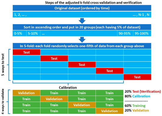
Figure 3.
Schematic of the dataset grouping and partitioning with the adjusted k-fold process.
- The runoff data were sorted by magnitude in ascending order.
- The sorted data were split into 20 groups, each encompassing 5% of the data.
- An almost equal portion of data from the groups was then moved randomly to each fold, so that all data within the groups were distributed to all folds at the end. A total of 205 monthly data (from 22 August 2000 to 22 September 2017 equivalent to 01/06/1379–31/06/1396 in Solar Hijri calendar) was categorized into 20 groups of 10 or 11 members. Then, almost one-kth of the groups’ members was allocated to each fold.
- After distributing the data to the folds using above steps, iterative partitioning started with taking the first fold for testing. Then, k – 1 different ways were possible for choice of another fold (2, 3, 4, or 5) for validation, and remaining k − 2 folds were eventually used for training, without a degree of freedom.
- For each iteration of k, having a constant fold chosen for testing, modelling was calibrated k – 1 (for different variation/ways of training-validation combinations) multiplied by 420 (for different combinations of hidden layers and neurons) multiplied by 10 (for different random parameter initialization) times. While the parameterization of each of the (k − 1) × 420 × 10 models was based on a minimum MSE for validation, they were additionally ranked based on the six performance criteria for calibration. For generalization of the output, a hybrid of the six best-ranked ANN models in the form of an arithmetic average was considered as final model for iteration k.
- The previous steps were continued k times so that, eventually, there were k hybrid models with different testing partitions to evaluate their outputs with the observed runoff. Selection of the best hybrid model was based on the comparison of their performances in both calibration and testing partitions of the runoff data.
3.3. Input Data Combinations for Conceptualized Data-Driven Modelling
Taking advantage of the spatially distributed RS data, seasonality in the observed monthly runoff and estimated monthly satellite precipitation data, and simple concepts affecting the rainfall–runoff process, different combinations, and organization of input variables were developed. The basic RS-based inputs were spatially averaged catchment-scale monthly GPM-IMERG-Late and MODIS-Terra data as introduced in Section 2.3 and Section 2.4. Thus, the following grid-based calculations were carried out first:
- –
- For ET (and PET), weighted sum of four or five consecutive 8-day time series data corresponding to their overlapping days within each month;
- –
- For NDVI and B7, weighted average of two consecutive monthly time series data corresponding to their overlapping days within each month;
- –
- For precipitation, sum of 29, 30, or 31 consecutive daily time series data in each month (note: water years in Iran starts with month 7 in Solar Hijri calendar and comprise five 30-day, one 29-day, and six 31-day months, except for leap years, where the sixth month is 30 days).
Then, the average of the resulting data for all grids from the above steps gave catchment-scale monthly RS-based data synced to the available monthly runoff data.
As mentioned in the introduction, two new types of input variables were formulated based on the satellite precipitation data. In fact, the spatially averaged monthly catchment precipitation could be related to any situation ranging from an isolated local event to a more distributed event covering the catchment. To investigate the areal variability of precipitation in the form of additional features that can explain the catchment response variation, rather than using too many input variables equivalent to the number of grids within a catchment, the following procedure was utilized:
- –
- First, the catchment-scale monthly precipitation (P) data were classified into 10 categories. For this purpose, they were sorted in an ascending order for each sub-catchment. The first category, with the smallest importance in producing runoff, was allocated to values between 0 and 2 mm/month, roughly encompassing 25% of the data depending on the sub-catchment. Remaining data (P > 2 mm/h) were first divided into eight additional categories with an almost equal data in each (roughly 9.4% of the data). In this way, however, the 9th category contained data with a wide range of values, including extremes. Thus, this category was further divided into two (roughly for percentiles 90–95 and 95–100) to avoid too long range of values in the 10th category.
- –
- Then, a set of areal precipitation coverage values was calculated using the ratio of the catchment area that received precipitation within the range specified by each category. Thus, the number of catchment-specific precipitation coverage ratios (CCOVs) as input variables was equal to the number of precipitation categories with 11 denominators of P as below (rounded values are presented here):
- ■
- Gamasiab (I): 0, 2, 8, 17, 24, 31, 38, 54, 82, 115, and 245;
- ■
- Qarasu (II): 0, 2, 9, 24, 33, 42, 51, 74, 126, 169, and 410;
- ■
- Seymareh (I–III): 0, 2, 9, 21, 31, 39, 52, 68, 108, 159, and 396;
- ■
- Kashkan (IV): 0, 2, 9, 20, 32, 48, 63, 82, 118, 212, and 629;
- ■
- Karkheh (I–V): 0, 2, 9, 23, 31, 43, 56, 73, 110, 157, and 410.
- –
- Next, in addition to CCOVs, another set of data was obtained by calculating the ratio of the catchment area that received higher than 50, 75, 100, 125, 150, and 200% of the P for each month (hereinafter, ECOVs).
Accordingly, ECOVs are event-specific variables with varying precipitation ranges from one month to another, whereas CCOVs are based on fixed precipitation categories for a given catchment. The sum of CCOVs and ECOVs for each month was equal to 1. Thus:
where for each catchment of size (=total number of GPM-IMERG grids, whose centres were located at the catchment’s border), and denote the number of grids that had a P in the th category as introduced above for the CCOVs and ECOVs, respectively.
Finally, based on the seasonality of precipitation and runoff data, outputs of two simple calculations were also used as input variables. Nash and Barsi [59] suggested that in catchments with seasonality/periodic signatures in runoff data, mean runoff can constitute a seasonal model. Further developments resulted in a linear perturbation model (LPM) as described in [25], where, instead of using actual runoff and precipitation, perturbations (departures) from the seasonal estimates of precipitation and runoff could be modelled. The output of such a perturbation model can be added to the output from the seasonal model to provide a hybrid modelling of runoff. Same theories were later employed in DD modelling of precipitation–runoff and referred to as non-linear perturbation model (NLPM), e.g., [40,60]. Such input is feasible to reduce the system complexity and improve the model efficiency of ANN models [60]. Accordingly:
- –
- One variable was a simple estimator of runoff using seasonal mean/model (SM) [59]:where y is runoff, d and r indicate date and year, respectively, and R is total number of years. In the adjusted k-fold process here, Rd is total repeats of month d in the calibration, and D is the cycle period (i.e., 12 for monthly data).
- –
- The other variable was precipitation perturbation (Pp) inspired from the notion of linear perturbation model [59,61]:where PSM is a seasonal model of P calculated such as Equation (8) using P instead of y.
A complete list of the input variable combinations is presented in Table 4. Finally, all input variables (Table 4) were introduced with 0–2-month lags (Lag 0–2) to evaluate possible patterns obtainable from the memory of the hydrological system. Then, the total length of the datasets used for modelling was two months smaller than the available common period of runoff and RS-based data. Regardless of the SM, combinations of the RS-based input variables in Table 4 could be considered in three classes depending on the affecting factors employed according to:
Table 4.
Combinations (Comb.) of input variables (P: precipitation; Pp: precipitation perturbation; ET: actual evapotranspiration; PET: potential evapotranspiration; NDVI: vegetation index NDVI; B7: MODIS Band 7; SM: seasonal mean runoff; CCOVs: coverage ratios of P for catchment-specific categories; ECOVs: coverage ratios of P for event-specific categories).
- A.
- Precipitation and potential ET (Comb. 1–4);
- B.
- Precipitation, potential ET, and NDVI (Comb. 5–8);
- C.
- Precipitation, potential ET, actual ET, NDVI, and B7 (Comb. 9–12).
3.4. Generalized Output of ANN
Overfitting is usually a cause of noisy output and larger errors when new data are presented to the model. As discussed earlier, cross-validation and verification, and early stopping were among the in-process ways of limiting overfitting. Another post-process way of coping with noisy output is to combine multiple models’ outputs for more generalized results. We used an arithmetic average of the six top-ranked models’ outputs based on six performance criteria (Table 3) within each iteration of a k-fold input–output problem (named hybrid model in Section 3.2).
4. Results
The k-fold process left 41, 41, and 123 pairs of input–output data for testing, validation, and training of the ANNs, respectively. Then, five hybrid models (arithmetic averages of the six top-ranked models in calibration based on the six performance criteria from Table 3), corresponding to the number of folds, were the result for a certain combination of input variables (Comb.) and the maximum lag time (1 or 2 months). Since all evaluated models under each combination of inputs had equal chance to take any of the folds for calibration and testing with many repeats of modelling (410 different ANN configurations per fold choice and 10 different random initial parameterizations per configuration), and the testing fold was always kept out of calibration, the hybrid model with the lowest RMSE in verification (test points) was considered to denote the best input combination, and, therefore, selected for further evaluations. Section 4.1, Section 4.2, Section 4.3, Section 4.4, Section 4.5 below represent the selected model results for the sub-catchments using time series hydrographs, and q–q plots. Additionally, the statistical results for the testing points were specifically compared to those obtained from a reference combination of inputs that did not use CCOVs and ECOVs but were still from the same class of inputs (i.e., Comb 1, 5, and 9 for input classes A, B, and C, respectively). Further discussions on inter-catchment comparisons of the spacetime precipitation variation and modelling performances are presented in the Discussion Section by comparing the values of the unitless statistical criteria for the entire dataset (calibration and testing) in the form of mean ± standard deviation (M ± SD).
4.1. Evaluation of Runoff Model for Gamasiab
Figure 4 shows the measured vs. modelled hydrographs (Figure 4a), as well as the q–q plots for calibration (Figure 4b) and testing (Figure 4c) of the selected model for Gamasiab. As seen in Figure 4a,c, the test data (cyan squares) were selected from all parts of the observed runoff distribution according to the adjusted k-fold process. Additionally, the selected model often accurately estimated the calibration and test points. For example, at two extreme values at month 7 of the years 4 and 18 (Figure 4a), the estimations matched the observations, although the later one was the highest value among the 205 months and was completely outside of the calibration data range. The general alignment of the observed and modelled runoff quantiles around the dashed 45-degree lines (Figure 4b,c) indicated an agreement between the statistical distribution of simulations and observations. However, some values around 100 MCM (million cubic meters) were underestimated in the test (Figure 4c).
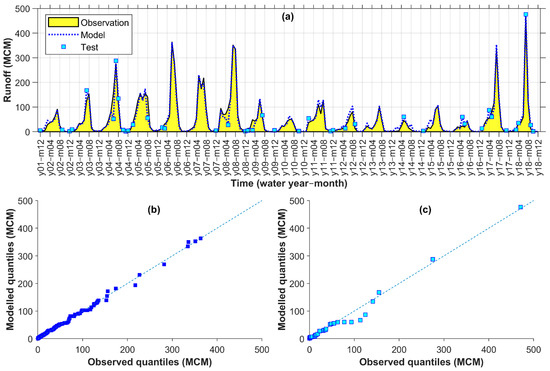
Figure 4.
Gamasiab observed vs. modelled monthly runoff time series (a) and q–q plots for calibration (b) and test (c) points (MCM: million cubic meters).
Table 5 represents the performance criteria values at test points for the selected hybrid model (versus a corresponding reference model from class B, i.e., Comb. 5 with Lag 0–2) under the input combination of Comb. 7 with Lag 0–2 for Gamasiab. Accordingly, the selected model showed PCC = 0.95, NSE = 0.90, KGE = 0.93, MAE = 16.12 (MCM), RAE = 0.30, and RMSE = 27.76 (MCM) in the testing points (Table 5). The PCC = 0.95 indicated a high linear correlation between the model and the observation. Additionally, NSE and KGE were slightly smaller than PCC, indicating that the components of bias in the mean and variance were small for this model. From the perfect and worst values of the criteria introduced in Table 3, the positive change rates of the first three criteria (PCC, NSE, and KGE) and negative change rates for the other ones (RMSE, RAE, and MAE) in Table 5 indicated favourable improvements by the selected model compared to the reference model. In other words, here, we could evaluate that the linear correlation (PCC) and efficiency (NES and KGE) increased and the magnitude (MAE and RMSE) and normalized (RAE) errors decreased using the selected model. Looking into some example values of changes, RMSE and RAE reduced by over 7 MCM/month and 19%, respectively, under Comb. 7 in relation to Comb. 5. Since the reference combination of inputs differed by that of the selected model only at the use of ECOVs for Gamasiab, we could attribute these favourable changes as an improvement due to the use of ECOVs for the monthly runoff modelling of the catchment. This improvement could reach 64% for NSE, while PCC and KGE improved by 25 and 26%, respectively. Such a difference could be related to the role of and existing in more components of the reformulation of the NSE in the form of as discussed in Section 3.1 [55], while they were only in one component of the KGE formula as presented in Table 3, regardless of PCC that exists in both.
Table 5.
Performance criteria values in test points for the selected (Comb. 7 Lag 0–2) vs. reference model (Comb. 5 Lag 0–2) for Gamasiab (RMSE and MAE are in million cubic meters, while the others are unitless) and the change rate (%) between them.
4.2. Evaluation of Runoff Model for Qarasu
The time series hydrographs and q–q plots in Figure 5 are related to the selected model for Qarasu. As seen in the cyan squares in Figure 5a, the selected model successfully estimated low to high values in most of the test points, including two high values in month 6 of year 7 and month 7 of year 8 (Figure 5a). Additionally, a generally good alignment was observed between the observed and modelled quantiles as well (Figure 5b,c).
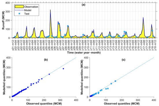
Figure 5.
Qarasu observed vs. modelled monthly runoff time series (a) and q–q plots for calibration (b) and test (c) points (MCM: million cubic meters).
As presented in Table 6, the selected model for Qarasu used inputs from Comb. 12 with Lag 0–1. This combination included both CCOVs and ECOVs as input variables. As a result, the statistical criteria for the test points using the selected model increased by rates of 1, 25, and 21% for PCC, NSE, and KGE, and decreased by 38, 30, and 35% for RMSE, RAE, and MAE, respectively, in comparison to the corresponding values from the reference model from class C (Comb. 9 Lag 0–1) that did not use any of the CCOVs or ECOVs as input variable.
Table 6.
Performance criteria for the selected (Comb. 12 Lag 0–1) vs. reference model (Comb. 9 Lag 0–1) in testing points for Qarasu (RMSE and MAE are in million cubic meters while the others are unitless) and the change rate (%) between them.
4.3. Evaluation of Runoff Model for Seymareh
The hydrographs and q–q plots in Figure 6 compare the observed runoff in Seymareh and simulations using the selected model that was obtained under Comb 7 with Lag 0–2 (Table 7). Although mostly aligned to the observations, some discrepancies appeared at calibration and test points of the selected hybrid model (Figure 6a). However, in the q–q plots, no obvious signature of over/under-estimation appeared in the outputs of the selected model.
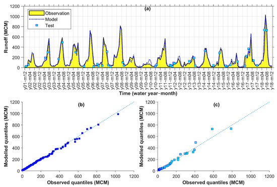
Figure 6.
Seymareh observed vs. modelled monthly runoff time series (a) and q–q plots for calibration (b) and test (c) points (MCM: million cubic meters).
Table 7.
Performance criteria values for the selected (Comb. 7 Lag 0–2) vs. reference model (Comb. 5 Lag 0–2) in testing points for Seymareh (RMSE and MAE are in million cubic meters while the others are unitless) and the change rate (%) between them.
Uniform decrease rates of −28% for MAE, RAE, and RMSE and an increase in the correlation and efficiency of the selected model compared to the reference in testing points (Table 7) ascertained that ECOVs improved monthly runoff modelling at Seymareh.
4.4. Evaluation of Runoff Model for Kashkan
For Kashkan, the selected model shows moderate to high discrepancies regarding both hydrographs and the q–q plots in Figure 7. For example, all three peak values in years 6–8 were underestimated while a few obvious overestimations of smaller values were observed in years 4, 7, and 14–16 (Figure 7a). Accordingly, a general tendency to underestimation and overestimation from the q–q plots at calibration (Figure 7b) and test (Figure 7c), respectively, may be a signature of the data inefficacy for the convergence of the monthly runoff modelling in Kashkan.
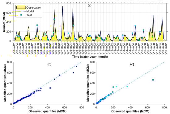
Figure 7.
Kashkan observed vs. modelled monthly runoff time series (a) and q–q plots for calibration (b) and test (c) points (MCM: million cubic meters).
Regardless of these discrepancies, the correlation value of PCC = 0.86 and the efficiency values of NSE = 0.73 and KGE = 0.77 among other criteria (Table 8) may indicate acceptable simulations when no better alternative data exist. Moreover, as observed in the final row of Table 8, all the criteria values improved after using the ECOVs through the selected model (Comb. 7 with Lag 0–1) compared to the corresponding reference model without ECOVs and CCOVs (Comb 5 with Lag 0–1). Noticeably low KGE and NSE for the reference model, may suggest that the ECOVs were still quite useful for improving the simulations of runoff in Kashkan. Thus, perhaps better results could be expected for Kashkan if longer data were available for the modelling. Possible underlying reasons for the rather poor modelling of Kashkan are discussed in Section 5.
Table 8.
Performance criteria values for the selected (Comb. 7 Lag 0–1) vs. reference model (Comb. 5 Lag 0–1) in testing points for Kashkan (RMSE and MAE are in million cubic meters while the others are unitless) and the change rate (%) between them.
4.5. Evaluation of Runoff Model for Karkheh
The entire study area of KRB received the majority of its runoff from the sub-catchments that were discussed so far in the Results section. Thus, the runoff modelling resulted in a somewhat average performance for the sub-catchments, i.e., somewhere in between the performances observed for Seymareh and Kashkan (compare Figure 6 and Figure 7 with Figure 8). For example, a rather smaller number and amount of model–observation discrepancies were observed in the time series hydrograph of Karkheh (Figure 8a) in comparison to Kashkan (Figure 7a), although there were still underestimations of two extreme data in month 6 of year 6 and month 7 of year 18 and some overestimations such as those in years 12 and 16 could be seen (Figure 8a). Additionally, looking into the q–q plots, the discrepancies were mostly limited to the test points (Figure 8c). As in Table 9, the best model for Karkheh was obtained under Comb. 12 with Lag 0–2, so it used the most complete input variable collection among the studied catchment areas. Like other sub-catchments, satellite precipitation coverage ratios (here, both CCOVs and ECOVs) again improved all statistical criteria values although, this time, the reference model (Comb. 9 with Lag 0–2) had generally closer performance criteria values to those of the best model with generally smaller change rates calculated in the final row of Table 9.
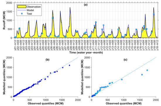
Figure 8.
Karkheh observed vs. modelled monthly runoff time series (a) and q–q plots for calibration (b) and test (c) points (MCM: million cubic meters).
Table 9.
Performance criteria for the selected (Comb. 12 Lag 0–2) vs. reference model (Comb. 9 Lag 0–2) in testing points for Karkheh (RMSE and MAE are in million cubic meters while the others are unitless) and the change rate (%) between them.
5. Inter-Catchment Comparisons and Discussions
Results of the best hybrid model per sub-catchment were discussed in the previous Section. Here, is a further discussion on the results of the catchments. In summary, for every catchment, a combination from class B or C of the input variables (Table 4) with a max lag time of 1 or 2 months resulted in the best modelling according to:
- –
- For Gamasiab (Section 4.1), Comb. 7 with Lag 0–2;
- –
- For Qarasu (Section 4.2), Comb. 12 with Lag 0–1;
- –
- For Seymareh (Section 4.3), Comb. 7 with Lag 0–2;
- –
- For Kashkan (Section 4.4), Comb. 7 with Lag 0–1;
- –
- For Karkheh (Section 4.5), Comb. 12 with Lag 0–2.
From the Lags, it can be inferred that the memory of the hydrologic system, concerning the influence of the previous state of input variables, was longer for Gamasiab, Seymareh, and Karkheh (catchment sizes > 11,000 km2) than for Qarasu and Kashkan (catchment sizes < 10,000 km2), which is reasonable due to the higher storage capacity in larger catchments. However, the best combination of input variables was Comb. 12 for both the smallest (Qarasu) and the largest (Karkheh) catchment, while Comb. 7 was best for other sub-catchments. Referring to Table 4, Comb. 12 from class C incorporated B7 and ET as additional variables compared to Comb. 7 from class B that incorporated ECOVs in addition to the catchment-scale basic variables in class A and B. Further investigations showed that the ECOVs for Qarasu were more useful than in Karkheh as the second-best performing model for Qarasu was obtained under Comb. 11, while it was Comb. 9 for Karkheh.
In general, the difference in the best combination of input variables for different sub-catchments can be interpreted in two ways: the inadequacy of the coverage ratios or necessity to include ET and B7. Among the catchments, Kashkan and Gamasiab had the weakest and strongest modelling performance, respectively, based on RAE, CC, NSE, and KGE that are unitless performance criteria, so comparable in different catchment areas. RAE was 0.5 and 0.3, CC was 0.86 and 0.95, NSE was 0.73 and 0.90, and KGE was 0.77 and 0.93 in the testing of the best selected models for Kashkan (Table 8) and Gamasiab (Table 5), respectively. Looking into the boxplots presented in Figure 9, these two catchments had the highest and lowest variation of P, respectively. Therefore, the weaker performance for Kashkan may be related to the insufficient calibration limited by the length of the satellite data. Such a lower performance of runoff modelling in Kashkan (compared to the other KRB sub-catchments) was also reported in the previous studies using other modelling types, such as the HBV model, and ground observations of precipitation [42].
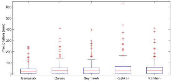
Figure 9.
Monthly P data variability for the KRB sub-catchments using GPM-IMERG-Late data. For each box, the central red line indicates median, and the bottom and top of the box indicate 1st and 3rd quartiles (q1 and q3), respectively. Whiskers denote the most extreme values not considered outliers ‘+’ as data points whose distance to q3 was more than 2.7 × SD × (q3–q1).
In addition to the temporal variability of P (Figure 9) and the size of the catchments discussed above, Figure 10 provides a useful ground to discuss the spatial variability of precipitation around the observed differences between the selected input variables for the sub-catchments as well as the inter-catchment differences of the performance criteria. Figure 10a–c depicts the mean, maximum, and coefficient of variation (CV) of the grid-based precipitation over the sub-catchments. According to Figure 10a, the highest average precipitation was in the western edges of segment III in Seymareh and in south and eastern Kashkan (IV). However, the highest and lowest spread of high CV (Figure 10c) was obtained for Kashkan (IV) and Gamasiab (I), respectively. These two sub-catchments were similar in size (Table 1). Thus, it seems that variability in precipitation was the most important factor in modelling performance. Regardless of this variability, however, incorporating ECOVs improved runoff modelling for all sub-catchments (Section 4). Particularly for Kashkan (Section 4.4), the highest change rates as above 240–280% for NSE and KGE in testing of the selected hybrid model compared to the reference model (Table 8) suggested an even higher added value from the satellite precipitation coverage ratios when the runoff modelling was complex due to the high spacetime precipitation variability.
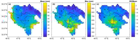
Figure 10.
Grid-based mean (a), maximum (b), and coefficient of variation (c) of monthly precipitation from GPM-IMERG-Late over Gamasiab (I), Qarasu (II), Seymareh (I–III), Kashkan (IV), and the entire study area of KRB (I–V).
Further evaluation of the added value of including precipitation coverage ratios could be based on the results of the mean ± standard deviation (M ± SD) of the performance criteria from all five hybrid models. Table 10 summarizes such values calculated from the entire length of data (calibration and test) to obtain more generalized results (compared to the condition of using only a single model and test data as in Section 4).
Table 10.
M ± SD values of the four unitless performance criteria for the hybrid models under the best (selected) and reference combination of the input variables and max lag time for different catchments (Gamasiab, Qarasu, Seymareh, Kashkan, and Karkheh).
Accordingly, a smaller SD at optimal M (i.e., minimum RAE or maximum PCC, NSE, and KGE) implied more robust runoff modelling regardless of data partitioning. For instance, in Gamasiab, the M value for KGE in the reference combination of inputs (Comb. 5 with Lag 0–2) was 0.87, while it was 0.93 under the best combination of inputs (Comb. 7 with Lag 0–2), and their corresponding SD was 0.07 and 0.03, respectively (Table 10). The lower SD under Comb. 7 (e.g., ±0.03 for KGE) compared to Comb. 5 (e.g., ±0.07 for KGE) implied a robust modelling for Gamasiab when ECOVs (Comb. 7) were combined with the catchment-scale input variables (i.e., P, PET, NDVI, and SMs). As in Table 10, the highest SD values for different performance criteria from the best combination of inputs were observed in Kashkan among all sub-catchments. In addition, while M values were generally higher (improved) for the best combination of inputs in comparison to the reference inputs for all catchments, the SD values for Kashkan increased (worsened). These facts indicated a higher dependency of the modelling performance on the data folds used for calibration and verification portions of this catchment compared to others. Therefore, as it was suggested before in Section 4.4, it can be assumed that longer data series are needed to fundamentally improve the modelling of runoff at a catchment with a high spacetime variability of precipitation using a satellite-based precipitation coverage ratio. In this study, GPM-IMERG products were available from mid-2000.
6. Conclusions and Remarks on Future Research Directions
The study formalized new input variables based on the gridded RS-based data and simple hydrological notions for better modelling of catchment response to precipitation with a conceptualized AI-assisted DD approach, primarily useful in sparsely gauged catchments. Backpropagation feed-forward ANNs, widely used in hydrological modelling, was used as the reference DD model. Each of the employed input–output combinations was calibrated and tested using an adjusted cross-validation and verification process to minimize overfitting. To assure achieving outputs with a reliable degree of generalization, many network configurations were evaluated for each combination of input–output variables. Eventually, multiple hybrid models from the best-ranked single models were selected for five case studies of the KRB with different catchment sizes between 5000 and 43,000 km2. As a result, the best runoff model for all catchments relied on an input variable combination that incorporated ECOVs (or both CCOVs and ECOVs) together with some reference input variable combinations. From the inter-catchment comparison, it was shown that, regardless of the catchment size, the best and worst performance criteria were obtained for Gamasiab and Kashkan, having the lowest and the highest spacetime precipitation variation, respectively. More interestingly, for Kashkan, the improvement of the performance scores by incorporating the precipitation coverage ratios, compared to the condition without the coverage ratios, was the highest among all sub-catchments. However, the performance of modelling in Kashkan showed a higher dependency on the data portions used for calibration and verification. Thus, while the highest degree of usefulness (from test data) was observed for the most challenging catchment in the sense that it had the highest variability of precipitation, a longer data length would be needed for generally better-performing model development in such catchments. On the contrary, the lowest degree of usefulness was for the largest catchment area, the entire study area of Karkheh.
The general hypothesis for calculating the areal coverage ratios of precipitation was that not only the average precipitation over the catchment but also its spatial distribution contributes to the runoff variation. This was reasonable to assume but it is important to note that CCOVs and ECOVs do not directly explain the location of precipitation. Instead, they consider the areal coverage ratios of precipitation with a possible correlation with the spacetime patterns of precipitation. For example, the underlying stratiform, rather than convective/orographic, precipitation events (typically representing slight to moderate intensities of precipitation over larger areas and durations) can be reflected as a bigger coverage ratio (close to 1) at a few low precipitation categories (e.g., CCOV1 = 0.9 and CCOV2 = 0.8 while CCOV9 = 0 and CCOV10 = 0). Conversely, the underlying convective precipitation events (typically representing local but intense rains) can be reflected as a higher coverage ratio at a few high precipitation categories (e.g., CCOV1 = 0 and CCOV2 = 0 while CCOV9 = 0.2 and CCOV10 = 0.1). Thus, CCOVs and ECOVs are only considered as additional inputs to DD models that can indirectly compensate for the lack of input data variability challenging lumped precipitation–runoff modelling. Anyway, the CCOVs and ECOVs introduced here were successful in all the studied catchments based on all the six performance criteria values. Thus, most likely, they can be useful in other study areas as well since they were formulized as catchment-specific and event-specific ratios. Some variation, such as a different categorization of precipitation data, might be needed depending on, e.g., how big the catchment is, how wet the climate is, and how long the available observation data are. For example, ECOVs contained six event-dependant variables, while CCOVs were based on ten catchment-specific categories, and the ECOVs were generally more useful than the CCOVs. The reason could be related to the presence of a small variation per a higher number of categories for training when the record is short. How long data should be used can also depend on the total variability of the dataset.
A similar methodological variation can be imagined for the adjusted cross-validation and verification process, although the general idea can be as that was used here. For example, the testing data sample larger for a 5-fold process (than for a 10-fold process) could help to ensure the robustness of the developed model in future uses. A 10-fold process, however, allows more data in calibration that could result in a better model. Therefore, a reasonable strategy can be to first use the 5-fold process and, then, depending on if the calibration needs improvement, the 10-fold process could also be evaluated.
In conclusion, regardless of the possible methodological variation, the shown usefulness of areal precipitation coverage-based variables here suggested new conceptualization potentials to leverage the increasingly advancing DD methods and satellite RS data in rainfall–runoff modelling, along with the use of physically-based (or conceptual) models. One of the strengths of AI-assisted DD modelling, such as ANN algorithms, is the ability to combine different inputs and apply multiple time lags with the automatization of modelling under a different architecture, which is not often the case for regular hydrological modelling. In addition, physically-based (or conceptual) modelling is not an ideal tool for the direct modelling of monthly runoff as its underlying concept such as the UH theory is usually built to relate precipitation and runoff data at an event scale and, then, the monthly runoff estimates are accumulated, e.g., from the initial daily estimates. These issues may result in computationally expensive modelling using regular physically-based (or conceptual) hydrological models when large-scale simulations need to evolve in accordance with the advancing worldwide satellite observations.
Finally, such as in any hydrological study relying on indirect estimations and modelling, the methodology introduced here is subject to uncertainty. Probably, the most important aspect is related to the limited length of the datasets due to the use of generally new satellite data (from 2000). There are obvious benefits of the new input variables used here; however, reliance on the model as well depends on the long-term representativity of the data. Developing a model using available data may still be useful for locations without an alternative that is a valid situation for many data-scarce catchments. As a technical note, the practical application of the modelling as described here can result in an error when the observed catchment-scale precipitation (P) in a month is greater than the higher edge of the final category of P for a catchment, and the model relies on CCOVs. To avoid such errors, the higher edge of the final category should be monitored. Another issue is related to the RS-based input variables used in the study, as well as the selection of what satellite product to use. The GPM is an advanced satellite precipitation mission that has gained interest in recent research of satellite precipitation after its precursor TRMM. GPM-IMERG data are now expanded to the same time span as for TRMM and presented in a few products at different temporal resolutions and data access latencies. Deciding which of the IMERG-Final or IMERG-Late products (probably the most useful ones here) is better to use for a region needs thorough investigations. As we discussed in the Introduction Section, these RS data are subject to errors, but it is not a straightforward task to adjust the biased data using the usually sparse ground observations, particularly in data-scarce catchments that will perhaps benefit most from the methodology. Therefore, using both ground-based and satellite-based data as separate input variables might be a better approach than adjusting satellite data in all grids from a local relation obtained at a few grids containing the sparse in situ stations, for instance. This study focused on monthly runoff modelling and used monthly input variables. The benefits of using direct monthly data for strategic surface water management were discussed in the previous paragraph. However, daily data are also interesting for other purposes where, for example, sub-monthly data are important. It has been noted that the methodology introduced here needs more investigations. Additionally, it is worth mentioning that some of the RS-based inputs used in this study (e.g., ET) were only available at 8-day and 16-day resolutions (at highest) that may not be favourable for daily modelling.
Author Contributions
Conceptualization, S.H.H.; Data curation, S.H.H.; Formal analysis, S.H.H.; Funding acquisition, S.H.H., H.H., A.F.F. and R.B.; Investigation, S.H.H.; Methodology, S.H.H.; Project administration, S.H.H., H.H., A.F.F. and R.B.; Resources, H.H., A.F.F. and R.B.; Software, S.H.H.; Supervision, H.H., A.F.F. and R.B.; Validation, S.H.H.; Visualization, S.H.H.; Writing—original draft, S.H.H.; Writing—review and editing, S.H.H., H.H., A.F.F. and R.B. All authors have read and agreed to the published version of the manuscript.
Funding
This research received no external funding.
Institutional Review Board Statement
Not applicable.
Informed Consent Statement
Not applicable.
Data Availability Statement
The study does not report any data. The data used for the method development in the study were introduced in Section 2.2, Section 2.3, Section 2.4 of the paper, and are available from the data owner’s website as acknowledged below with citations.
Acknowledgments
The runoff data were obtained from the office of Basic Water Resources Studies, Iran Water Resources Management Company [62]. The MODIS Terra data were obtained from the MOD16A2v006 and MOD13A3v006 products of NASA [63,64]. The GPM-IMERG data were obtained from the GPM_3IMERGDL product of NASA [65]. The ANN models and all figures were produced by MATLAB R2020a with a licence provided by Lund University.
Conflicts of Interest
The authors declare no conflict of interest.
References
- Hosseini, S.H. Disastrous Floods after Prolonged Droughts Have Challenged Iran. FUF-Bladet. 2019, pp. 30–32. Available online: https://portal.research.lu.se/en/publications/disastrous-floods-after-prolonged-droughts-have-challenged-iran (accessed on 22 November 2021).
- Boafo, Y.A.; Saito, O.; Jasaw, G.S.; Yiran, G.A.B.; Lam, R.D.; Mohan, G.; Kranjac-Berisavljevic, G. Perceived Community Resilience to Floods and Droughts Induced by Climate Change in Semi-arid Ghana. In Sustainability Challenges in Sub-Saharan Africa I: Continental Perspectives and Insights from Western and Central Africa; Gasparatos, A., Ahmed, A., Naidoo, M., Karanja, A., Fukushi, K., Saito, O., Takeuchi, K., Eds.; Springer: Singapore, 2020; pp. 191–219. [Google Scholar] [CrossRef]
- Prama, M.; Omran, A.; Schroder, D.; Abouelmagd, A. Vulnerability assessment of flash floods in Wadi Dahab Basin, Egypt. Environ. Earth Sci. 2020, 79, 17. [Google Scholar] [CrossRef] [Green Version]
- Ward, F.A.; Amer, S.A.; Ziaee, F. Water allocation rules in Afghanistan for improved food security. Food Secur. 2013, 5, 35–53. [Google Scholar] [CrossRef]
- Gohari, A.; Eslamian, S.; Mirchi, A.; Abedi-Koupaei, J.; Bavani, A.M.; Madani, K. Water transfer as a solution to water shortage: A fix that can backfire. J. Hydrol. 2013, 491, 23–39. [Google Scholar] [CrossRef]
- Deng, C.; Liu, P.; Liu, Y.; Wu, Z.; Wang, D. Integrated hydrologic and reservoir routing model for real-time water level forecasts. J. Hydrol. Eng. 2015, 20, 05014032. [Google Scholar] [CrossRef]
- Hosseini, S.H.; Ghorbani, M.A.; Bavani, A.M. Impacts of Climate Change on Streamflow and Reservoir Operation. In Proceedings of The Second Regional Conference on Climate Change and Global Warming, Center for Research in Climate Change and Global Warming (CRCC), Institute for Advanced Studies in Basic Sciences, Zanjan, Iran, 12 November 2014. [Google Scholar]
- Saeidabadi, R.; Najafi, M.S.; Roshan, G.; Fitchett, J.M.; Abkharabat, S. Modelling spatial, altitudinal and temporal variability of annual precipitation in mountainous regions: The case of the Middle Zagros, Iran. Asia-Pac. J. Atmos. Sci. 2016, 52, 437–449. [Google Scholar] [CrossRef]
- Hiebl, J.; Frei, C. Daily precipitation grids for Austria since 1961—development and evaluation of a spatial dataset for hydroclimatic monitoring and modelling. Theor. Appl. Climatol. 2018, 132, 327–345. [Google Scholar] [CrossRef]
- Gilewski, P.; Nawalany, M. Inter-comparison of rain-gauge, radar, and satellite (IMERG GPM) precipitation estimates performance for rainfall-runoff modeling in a mountainous catchment in Poland. Water 2018, 10, 1665. [Google Scholar] [CrossRef] [Green Version]
- Gilewski, P. Impact of the Grid Resolution and Deterministic Interpolation of Precipitation on Rainfall-Runoff Modeling in a Sparsely Gauged Mountainous Catchment. Water 2021, 13, 230. [Google Scholar] [CrossRef]
- Young, C.-C.; Liu, W.-C. Prediction and modelling of rainfall–runoff during typhoon events using a physically-based and artificial neural network hybrid model. Hydrol. Sci. J. 2015, 60, 2102–2116. [Google Scholar] [CrossRef]
- Carcano, E.C.; Bartolini, P.; Muselli, M.; Piroddi, L. Jordan recurrent neural network versus IHACRES in modelling daily streamflows. J. Hydrol. 2008, 362, 291–307. [Google Scholar] [CrossRef]
- Smith, J.; Eli, R.N. Neural-network models of rainfall-runoff process. J. Water Resour. Plan. Manag. 1995, 121, 499–508. [Google Scholar] [CrossRef]
- Dawson, C.; Wilby, R. Hydrological modelling using artificial neural networks. Prog. Phys. Geogr. 2001, 25, 80–108. [Google Scholar] [CrossRef]
- Yilmaz, A.; Imteaz, M.; Jenkins, G. Catchment flow estimation using Artificial Neural Networks in the mountainous Euphrates Basin. J. Hydrol. 2011, 410, 134–140. [Google Scholar] [CrossRef]
- Ghorbani, M.A.; Hosseini, S.H.; Fazelifard, M.H.; Abbasi, H. Sediment load estimation by MLR, ANN, NF and sediment rating curve (SRC) in Rio Chama river. J. Civ. Eng. Urban. 2013, 3, 136–141. [Google Scholar]
- Kang, B.; Ku, Y.H.; Do Kim, Y. A case study for ANN-based rainfall–runoff model considering antecedent soil moisture conditions in Imha Dam watershed, Korea. Environ. Earth Sci. 2015, 74, 1261–1272. [Google Scholar] [CrossRef]
- Yang, T.; Asanjan, A.A.; Welles, E.; Gao, X.; Sorooshian, S.; Liu, X. Developing reservoir monthly inflow forecasts using artificial intelligence and climate phenomenon information. Water Resour. Res. 2017, 53, 2786–2812. [Google Scholar] [CrossRef]
- Pradhan, P.; Tingsanchali, T.; Shrestha, S. Evaluation of Soil and Water Assessment Tool and Artificial Neural Network models for hydrologic simulation in different climatic regions of Asia. Sci. Total Environ. 2020, 701, 134308. [Google Scholar] [CrossRef]
- Wei, C.-C. Comparison of River Basin Water Level Forecasting Methods: Sequential Neural Networks and Multiple-Input Functional Neural Networks. Remote Sens. 2020, 12, 4172. [Google Scholar] [CrossRef]
- Beck, M.B. Forecasting environmental change. J. Forecast. 1991, 10, 3–19. [Google Scholar] [CrossRef]
- Kachroo, R. River flow forecasting. Part 1. A discussion of the principles. J. Hydrol. 1992, 133, 1–15. [Google Scholar] [CrossRef]
- Paik, K.; Kim, J.H.; Kim, H.S.; Lee, D.R. A conceptual rainfall-runoff model considering seasonal variation. Hydrol. Processes Int. J. 2005, 19, 3837–3850. [Google Scholar] [CrossRef]
- Kachroo, R.; Liang, G. River flow forecasting. Part 2. Algebraic development of linear modelling techniques. J. Hydrol. 1992, 133, 17–40. [Google Scholar] [CrossRef]
- Vaze, J.; Post, D.; Chiew, F.; Perraud, J.-M.; Viney, N.; Teng, J. Climate non-stationarity–validity of calibrated rainfall–runoff models for use in climate change studies. J. Hydrol. 2010, 394, 447–457. [Google Scholar] [CrossRef]
- Hosseini, S.H.; Ghorbani, M.A.; Bavani, A.M. Raifall-runoff modelling under the climate change condition in order to project future streamflows of sufichay watershed. J. Watershed Manag. Res. 2015, 6, 1–14. [Google Scholar]
- Zareian, M.; Eslamian, S.; Gohari, A.; Adamowski, J. The effect of climate change on watershed water balance. In Mathematical Advances towards Sustainable Environmental Systems; Springer: Cham, Swizerlands, 2017; pp. 215–238. [Google Scholar]
- Ashofteh, P.S.; Bozorg-Haddad, O.; Loáiciga, H.A. Logical genetic programming (LGP) development for irrigation water supply hedging under climate change conditions. Irrig. Drain. 2017, 66, 530–541. [Google Scholar] [CrossRef]
- Yi, L.; Zhang, W.-C.; Yan, C.-A. A modified topographic index that incorporates the hydraulic and physical properties of soil. Hydrol. Res. 2017, 48, 370–383. [Google Scholar] [CrossRef]
- Musie, M.; Sen, S.; Srivastava, P. Comparison and evaluation of gridded precipitation datasets for streamflow simulation in data scarce watersheds of Ethiopia. J. Hydrol. 2019, 579, 124168. [Google Scholar] [CrossRef]
- Mo, C.; Zhang, M.; Ruan, Y.; Qin, J.; Wang, Y.; Sun, G.; Xing, Z. Accuracy Analysis of IMERG Satellite Rainfall Data and Its Application in Long-term Runoff Simulation. Water 2020, 12, 2177. [Google Scholar] [CrossRef]
- Roth, V.; Lemann, T. Comparing CFSR and conventional weather data for discharge and soil loss modelling with SWAT in small catchments in the Ethiopian Highlands. Hydrol. Earth Syst. Sci. 2016, 20, 921–934. [Google Scholar] [CrossRef] [Green Version]
- Hashemi, H.; Fayne, J.; Lakshmi, V.; Huffman, G.J. Very high resolution, altitude-corrected, TMPA-based monthly satellite precipitation product over the CONUS. Sci. Data 2020, 7, 1–10. [Google Scholar] [CrossRef]
- Maghsood, F.F.; Hashemi, H.; Hosseini, S.H.; Berndtsson, R. Ground Validation of GPM IMERG Precipitation Products over Iran. Remote Sens. 2020, 12, 48. [Google Scholar] [CrossRef] [Green Version]
- Chen, H.; Chandrasekar, V.; Cifelli, R.; Xie, P. A machine learning system for precipitation estimation using satellite and ground radar network observations. IEEE Trans. Geosci. Remote Sens. 2019, 58, 982–994. [Google Scholar] [CrossRef]
- Ramanujam, S.; Chandrasekar, R.; Chakravarthy, B. A new PCA-ANN algorithm for retrieval of rainfall structure in a precipitating atmosphere. Int. J. Numer. Methods Heat Fluid Flow 2011, 21, 1002–1025. [Google Scholar] [CrossRef]
- Chen, H.; Chandrasekar, V.; Tan, H.; Cifelli, R. Rainfall estimation from ground radar and TRMM precipitation radar using hybrid deep neural networks. Geophys. Res. Lett. 2019, 46, 10669–10678. [Google Scholar] [CrossRef]
- Ramanujam, S.; Radhakrishnan, C.; Subramani, D.; Chakravarthy, B. On the effect of non-raining parameters in retrieval of surface rain rate using TRMM PR and TMI measurements. IEEE J. Sel. Top. Appl. Earth Obs. Remote Sens. 2012, 5, 735–743. [Google Scholar] [CrossRef]
- Shoaib, M.; Shamseldin, A.Y.; Khan, S.; Khan, M.M.; Khan, Z.M.; Melville, B.W. A wavelet based approach for combining the outputs of different rainfall–runoff models. Stoch. Environ. Res. Risk Assess. 2018, 32, 155–168. [Google Scholar] [CrossRef]
- Kwon, M.; Kwon, H.-H.; Han, D. A Hybrid Approach Combining Conceptual Hydrological Models, Support Vector Machines and Remote Sensing Data for Rainfall-Runoff Modeling. Remote Sens. 2020, 12, 1801. [Google Scholar] [CrossRef]
- Kazemi, H.; Hashemi, H.; Maghsood, F.F.; Hosseini, S.H.; Sarukkalige, R.; Jamali, S.; Berndtsson, R. Climate vs. Human Impact: Quantitative and Qualitative Assessment of Streamflow Variation. Water 2021, 13, 2404. [Google Scholar] [CrossRef]
- Machado, F.; Mine, M.; Kaviski, E.; Fill, H. Monthly rainfall–runoff modelling using artificial neural networks. Hydrol. Sci. J.—J. Des Sci. Hydrol. 2011, 56, 349–361. [Google Scholar] [CrossRef]
- Garbrecht, J.D. Comparison of three alternative ANN designs for monthly rainfall-runoff simulation. J. Hydrol. Eng. 2006, 11, 502–505. [Google Scholar] [CrossRef] [Green Version]
- Huffman, G.J.; Bolvin, D.; Braithwaite, D.; Hsu, K.; Joyce, R.; Kidd, C.; Nelkin, E.; Sorooshian, S.; Tan, J.; Xie, P. Algorithm Theoretical Basis Document (ATBD) Version 4.5: NASA Global Precipitation Measurement (GPM) Integrated Multi-satellite Retrievals for GPM (IMERG); NASA: Greenbelt, MD, USA, 2015. [Google Scholar]
- Huffman, G.J.; Bolvin, D.T.; Braithwaite, D.; Hsu, K.; Joyce, R.; Kidd, C.; Nelkin, E.J.; Sorooshian, S.; Tan, J.; Xie, P. Algorithm Theoretical Basis Document (ATBD) Version 06: NASA Global Precipitation Measurement (GPM) Integrated Multi-Satellite Retrievals for GPM (IMERG); NASA: Greenbelt, MD, USA, 2019. [Google Scholar]
- Cotugno, A.; Smith, V.; Baker, T.; Srinivasan, R. A Framework for Calculating Peak Discharge and Flood Inundation in Ungauged Urban Watersheds Using Remotely Sensed Precipitation Data: A Case Study in Freetown, Sierra Leone. Remote Sens. 2021, 13, 3806. [Google Scholar] [CrossRef]
- Running, S.W.; Mu, Q.; Zhao, M.; Moreno, A. MODIS Global Terrestrial Evapotranspiration (ET) Product (MOD16A2/A3 and Year-End Gap-Filled MOD16A2GF/A3GF) NASA Earth Observing System MODIS Land Algorithm (For Collection 6); National Aeronautics and Space Administration: Washington, DC, USA, 2019. [Google Scholar]
- Didan, K.; Munoz, A.B.; Solano, R.; Huete, A. MODIS Vegetation Index User’s Guide (MOD13 Series); Vegetation Index and Phenology Lab, University of Arizona: Tucson, AZ, USA, 2015. [Google Scholar]
- Chu, D. MODIS remote sensing approaches to monitoring soil moisture in Tibet, China. Remote Sens. Lett. 2018, 9, 1148–1157. [Google Scholar] [CrossRef]
- Cigizoglu, H.K.; Kişi, Ö. Flow prediction by three back propagation techniques using k-fold partitioning of neural network training data. Hydrol. Res. 2005, 36, 49–64. [Google Scholar] [CrossRef]
- Kratzert, F.; Klotz, D.; Herrnegger, M.; Sampson, A.K.; Hochreiter, S.; Nearing, G.S. Toward improved predictions in ungauged basins: Exploiting the power of machine learning. Water Resour. Res. 2019, 55, 11344–11354. [Google Scholar] [CrossRef] [Green Version]
- Lee, J.-Y.; Choi, C.; Kang, D.; Kim, B.S.; Kim, T.-W. Estimating Design Floods at Ungauged Watersheds in South Korea Using Machine Learning Models. Water 2020, 12, 3022. [Google Scholar] [CrossRef]
- Hagan, M.; Demuth, H.; Beale, M.; De Jesus, O. Neural Network Design; PWS Publishing Company: Boston, MA, USA, 1996. [Google Scholar]
- Gupta, H.V.; Kling, H.; Yilmaz, K.K.; Martinez, G.F. Decomposition of the mean squared error and NSE performance criteria: Implications for improving hydrological modelling. J. Hydrol. 2009, 377, 80–91. [Google Scholar] [CrossRef] [Green Version]
- Pearson, K. Mathematical contributions to the theory of evolution—On a form of spurious correlation which may arise when indices are used in the measurement of organs. Proc. R. Soc. Lond. 1897, 60, 489–498. [Google Scholar]
- Nash, J.E.; Sutcliffe, J.V. River flow forecasting through conceptual models part I—A discussion of principles. J. Hydrol. 1970, 10, 282–290. [Google Scholar] [CrossRef]
- Legates, D.R.; McCabe, G.J., Jr. Evaluating the use of “goodness-of-fit” measures in hydrologic and hydroclimatic model validation. Water Resour. Res. 1999, 35, 233–241. [Google Scholar] [CrossRef]
- Nash, J.; Barsi, B.I. A hybrid model for flow forecasting on large catchments. J. Hydrol. 1983, 65, 125–137. [Google Scholar] [CrossRef]
- Pang, B.; Guo, S.; Xiong, L.; Li, C. A nonlinear perturbation model based on artificial neural network. J. Hydrol. 2007, 333, 504–516. [Google Scholar] [CrossRef]
- Kachroo, R.; Liang, G.; O’Connor, K. Application of the linear perturbation model (LPM) to flood routing on the Mekong River. Hydrol. Sci. J. 1988, 33, 193–214. [Google Scholar] [CrossRef] [Green Version]
- Monthly hydrological data from the office of Basic Water Resources Studies, IRAN Water Resources Management Company. Available online: https://wrbs.wrm.ir/ (accessed on 31 October 2021). (In Persian).
- Running, S.; Mu, Q.; Zhao, M. MOD16A2 MODIS/Terra Net Evapotranspiration 8-Day L4 Global 500 m SIN Grid V006 [Data set]. 2017. NASA EOSDIS Land Processes DAAC. Available online: https://doi.org/10.5067/MODIS/MOD16A2.006 (accessed on 31 July 2020).
- Didan, K. MOD13A3 MODIS/Terra vegetation Indices Monthly L3 Global 1 km SIN Grid V006. 2015. Distributed by NASA EOSDIS Land Processes DAAC. Available online: https://doi.org/10.5067/MODIS/MOD13A3.006 (accessed on 14 August 2020).
- Huffman, G.J.; Stocker, E.F.; Bolvin, D.T.; Nelkin, E.J.; Tan, J. GPM IMERG Late Precipitation L3 1 day 0.1 degree × 0.1 degree V06. 2019. Edited by Andrey Savtchenko, Greenbelt, MD, Goddard Earth Sciences Data and Information Services Center (GES DISC). Available online: https://doi.org/10.5067/GPM/IMERGDL/DAY/06 (accessed on 8 August 2020).


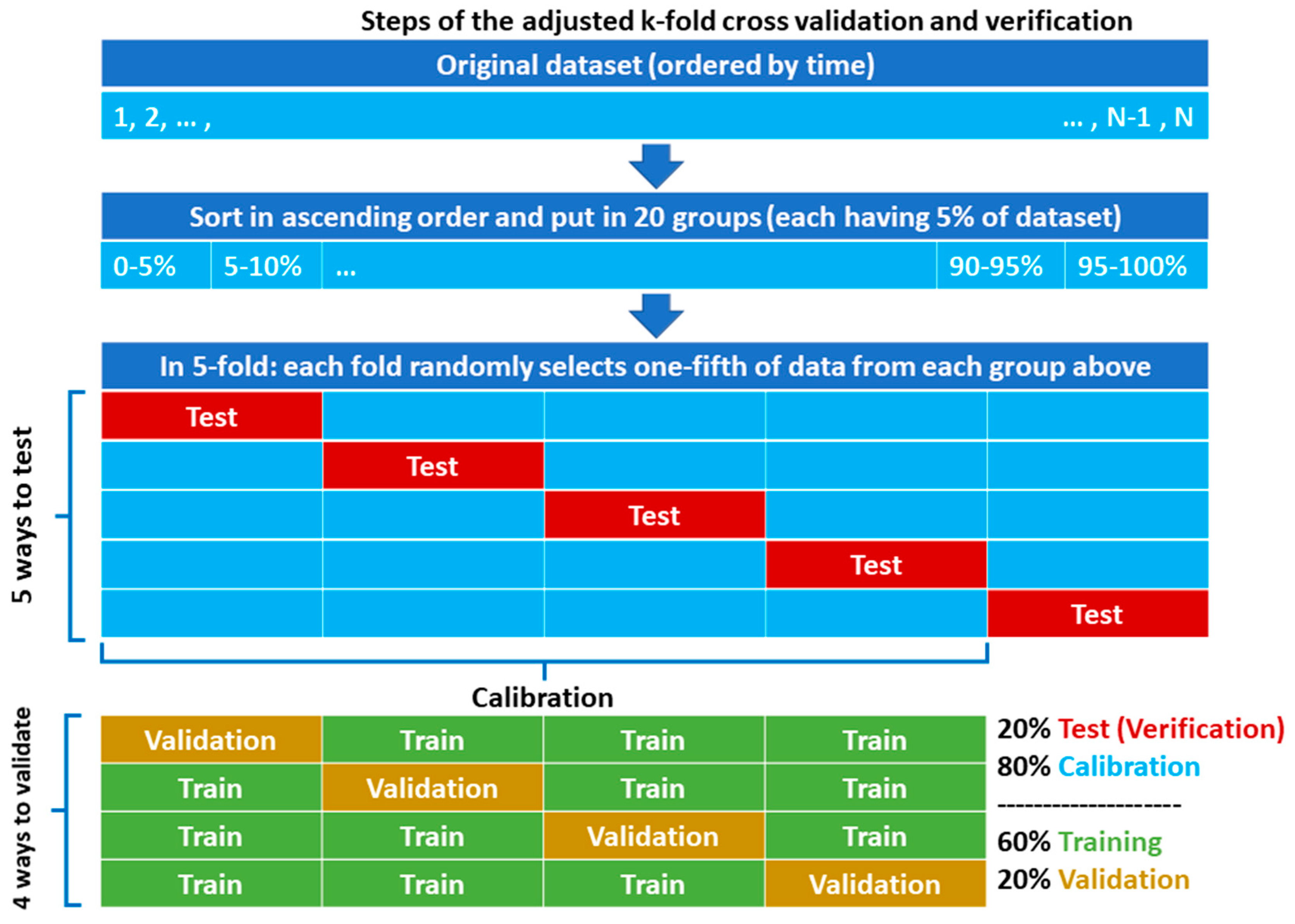
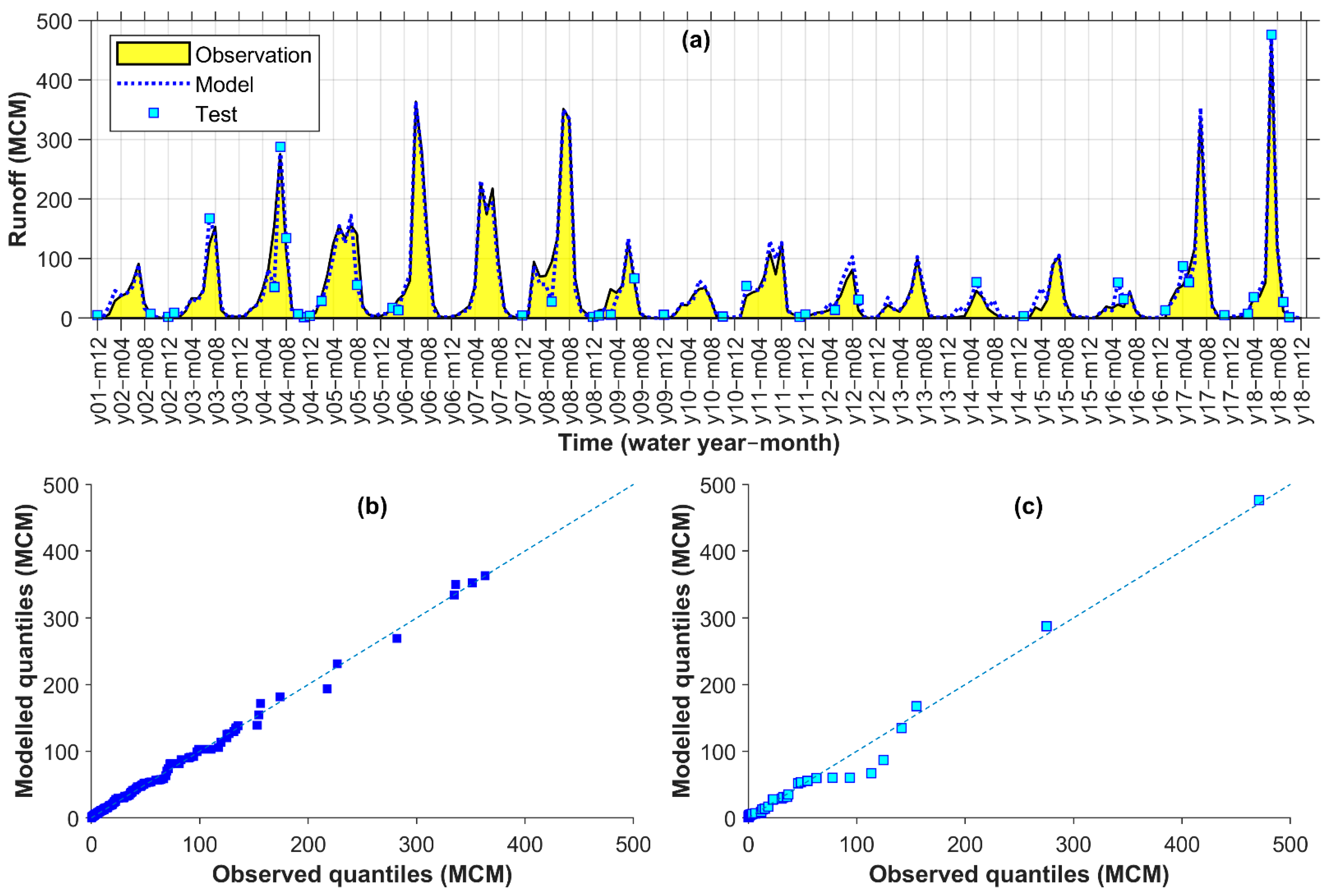
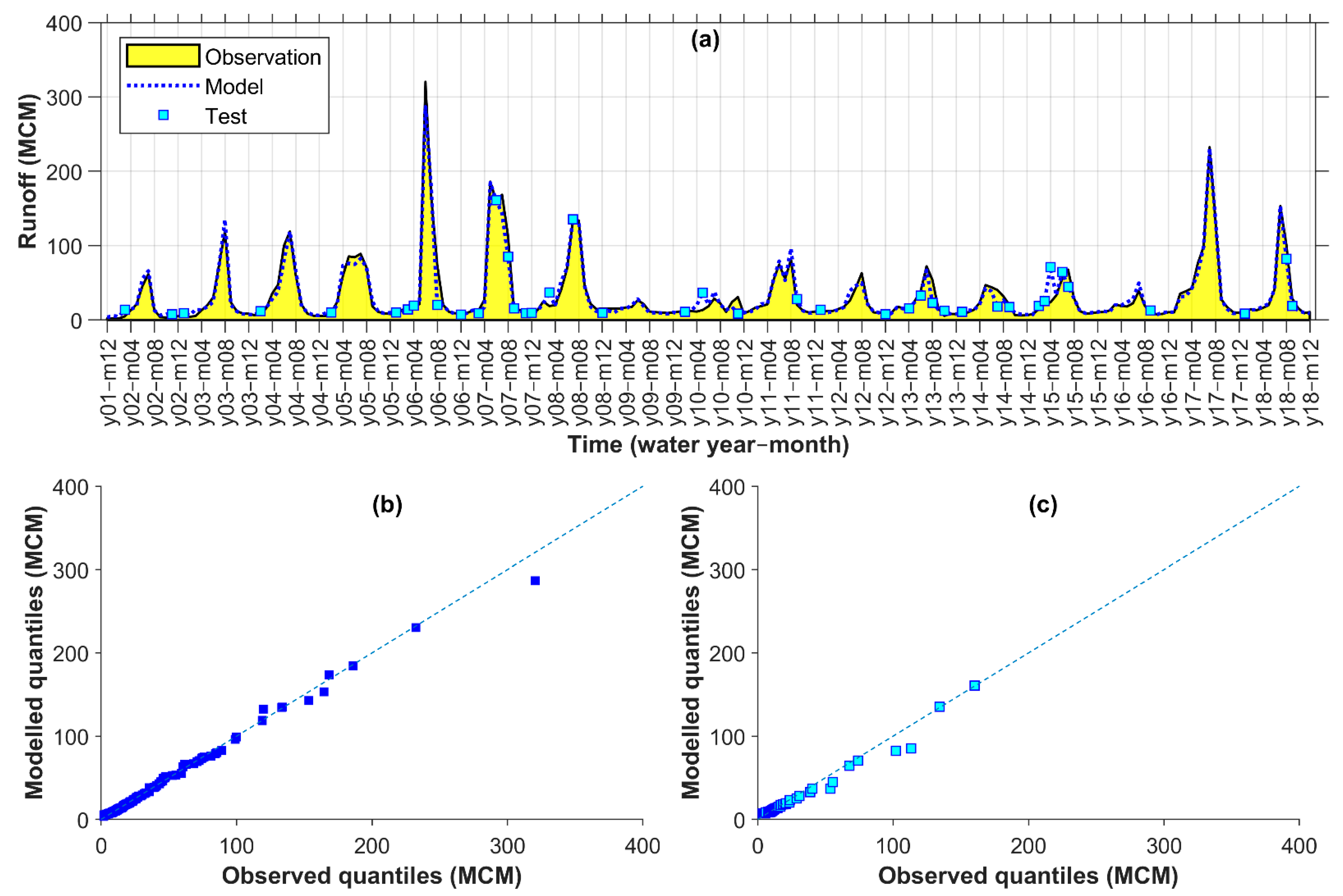
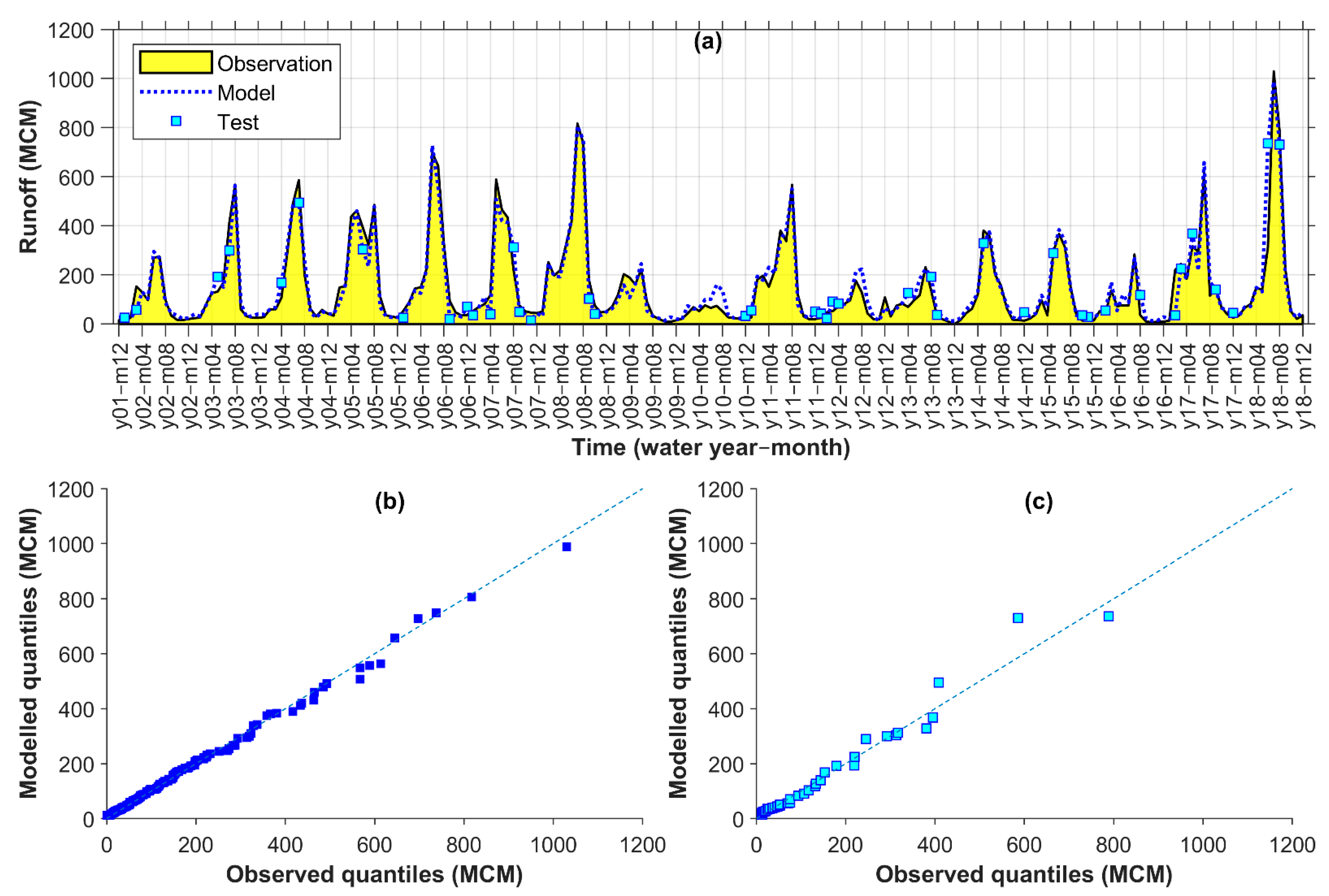
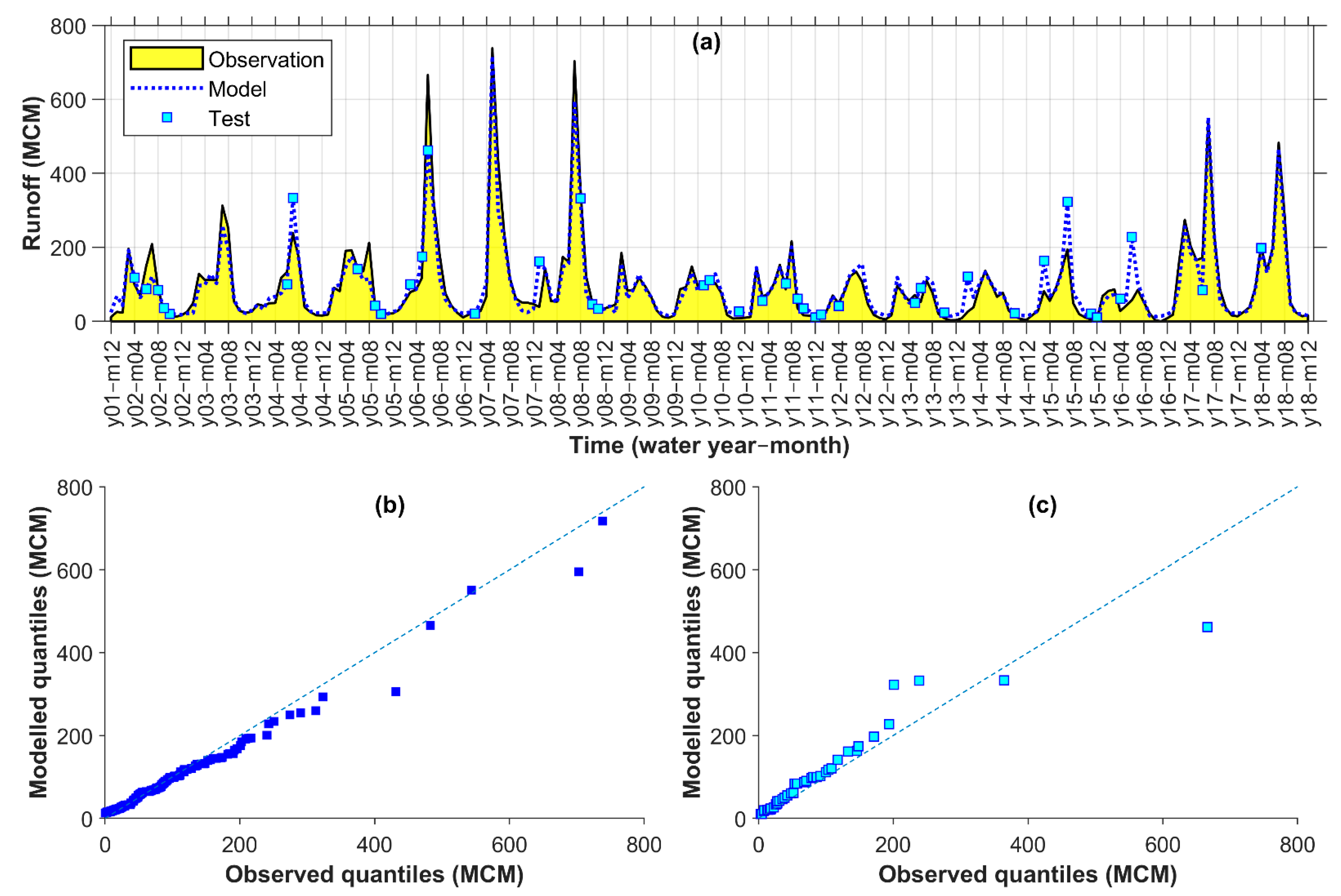

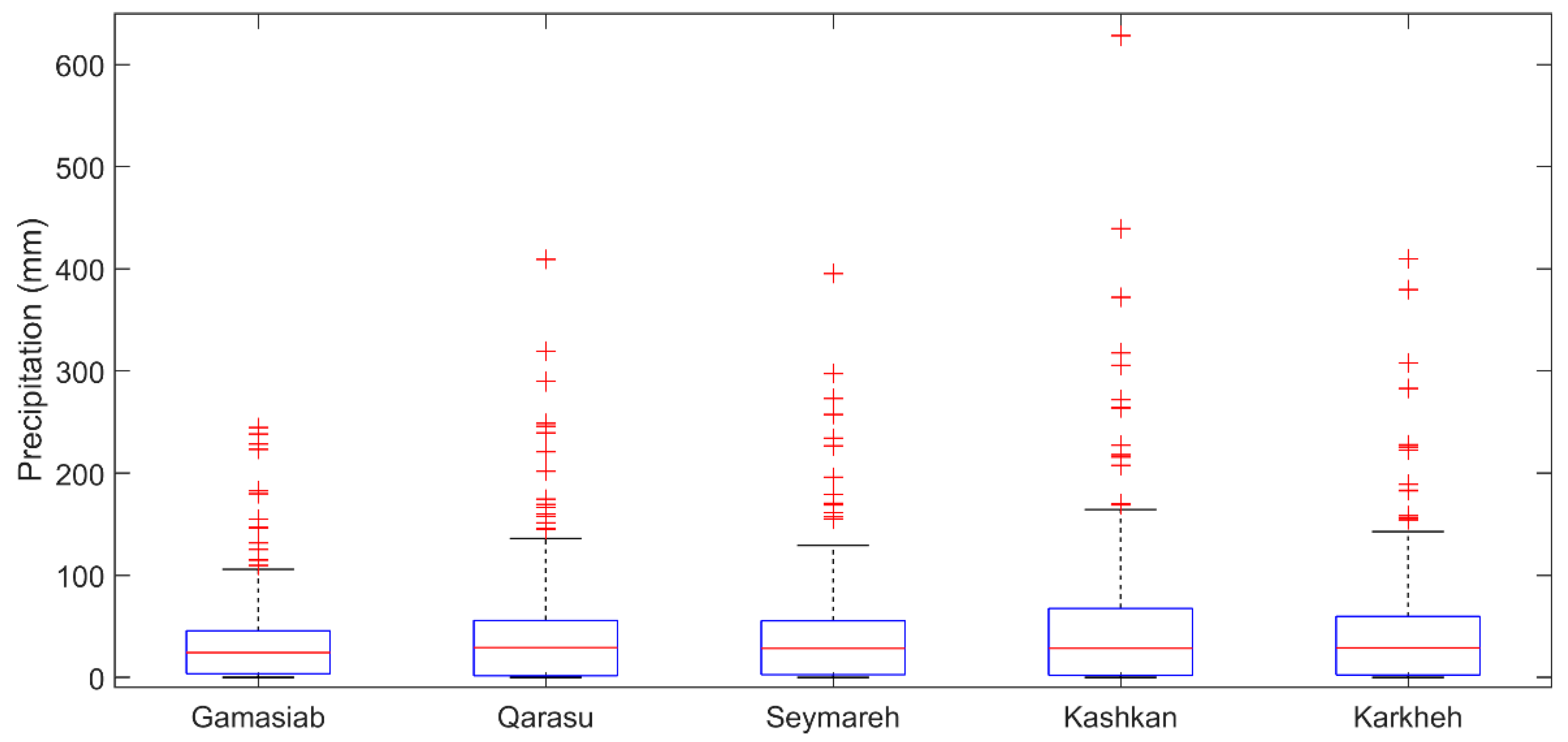

Publisher’s Note: MDPI stays neutral with regard to jurisdictional claims in published maps and institutional affiliations. |
© 2022 by the authors. Licensee MDPI, Basel, Switzerland. This article is an open access article distributed under the terms and conditions of the Creative Commons Attribution (CC BY) license (https://creativecommons.org/licenses/by/4.0/).