Abstract
The intensity of agricultural activities and the characteristics of water consumption affect the hydrological processes of inland river basins in Central Asia. The crop water requirements and water productivity are different between the Amu Darya and Syr Darya river basins due to the different water resource development and utilization policies of Uzbekistan and Kazakhstan, which have resulted in more severe agricultural water consumption of the Amu Darya delta than the Syr Darya delta, and the differences in the surface runoff are injected into the Aral Sea. To reveal the difference in water resource dissipation, water productivity, and its influencing factors between the two basins, this study selected the irrigation areas of Amu Darya delta (IAAD) and Syr Darya delta (IASD) as typical examples; the actual evapotranspiration (ETa) was retrieved by using the modified surface energy balance algorithm for land model (SEBAL) based on high spatial resolution Landsat images from 2000 to 2020. Land use and cover change (LUCC) and streamflow data were obtained to analyze the reasons for the spatio-temporal heterogeneity of regional ETa. The water productivity of typical crops in two irrigation areas was compared and combined with statistical data. The results indicate that: (1) the ETa simulated by the SEBAL model matched the crop evapotranspiration (ETc) calculated by the Penman–Monteith method and ground-measured data well, with all the correlation coefficients higher than 0.7. (2) In IAAD, the average ETa was 1150 mm, and the ETa had shown a decreasing trend; for the IASD, the average ETa was 800 mm. The ETa showed an increasing trend with low stability due to a large amount of developable cultivated land. The change of cultivated land dominated the spatio-temporal characteristics of ETa in the two irrigation areas (3). Combined with high spatial resolution ETa inversion results, the water productivity of cotton and rice in IAAD was significantly lower than in IASD, and wheat was not significantly different, but all were far lower than the international average. This study can provide useful information for agricultural water management in the Aral Sea region.
1. Introduction
Since 1960, the excessive utilization of the water resources of the Amu Darya and Syr Darya river basins has significantly reduced the amount of water inflow to the Aral Sea, resulting in a sharp shrinkage of the Aral Sea, a continuous decline in the lake level, and a deterioration of the ecological environment [1,2]. Studies have shown that agricultural intensification in the Amu Darya and Syr Darya river basins is the main cause of the crisis of the Aral Sea [3,4,5]. The increased demand for irrigation water has resulted in a significant reduction in inflow into the Aral Sea [2,6]. In 1987, the Aral Sea was divided into the northern Aral Sea and the southern Aral Sea. The construction of the Kokaral Dam blocked the water exchange between the southern and the northern Aral Sea, resulting in significant differences in water volume between the two parts of the lake [7,8]. In recent years, the level of the southern Aral Sea fed by the Amu Darya River has fallen sharply due to a significant reduction in the inflow, while the level of the northern Aral Sea, obtaining water from the Syr Darya river, has been increased with an increased inflow from 1987 to 2014 [2,5,9,10,11]. The areas of the northern and southern Aral Seas present different destinies, which not only reflect the difference in the inflows of Syr Darya and Amu Darya Rivers but also imply a difference in the intensity of agricultural activities in the delta regions of the two rivers. Particularly in the Amu Darya delta, the riparian forest along the Amu Darya River has been reclaimed for farmland, and a dam and reservoir were built in the Muynak area at the entrance of the South Aral Sea in 1982 to keep the water in the delta and meet the agricultural water demand. Since the 1990s, there has been no surface runoff directly into the South Aral Sea; the groundwater from the irrigation area in the delta region has become the main recharge source of the South Aral Sea [12,13,14,15]. However, the restoration and maintenance of the North Aral Sea have been an important goal of water resource management in the lower reaches of the Syr Darya river after the collapse of the Soviet Union. Therefore, it helps alleviate the crisis of the Aral Sea to explore the difference in agricultural water consumption and water productivity between the Amu and Syr deltas.
Crop evapotranspiration is a key aspect of efficient irrigation water management [16]. Traditional site ET observations include the Bowen ratio-energy balance method, photosynthesis instruments, weighing lysimeters, the eddy correlation method, and others [17,18,19,20], but these methods are limited by equipment, high cost, and point or field scale, and do not apply to the acquisition of ET in the irrigation areas in Central Asia with sparse observation networks. The calculation of crop water demand based on the Penman–Monteith formula can be used to map the actual evapotranspiration (ETa) of crops on a large scale, but this requires accurate crop structure information [21]. The water balance method can also calculate regional ET if other hydrological elements are available [22].
With the development of remote-sensing technology, techniques for mapping ET with few observed data have been developed. However, in the Aral Sea basin, the existing remote-sensing ET products have some limitations, such as the fact that the MOD16 products significantly underestimate ET in sparse vegetation areas [23], the Global Land Evaporation and Amsterdam Model (GLEAM), and Global Land Data Assimilation System (GLDAS) data are not adequate for the present study due to their coarse spatial resolution [24,25,26]. More recently, high-resolution ET products from the Ecosystem Spaceborne Thermal Radiometer Experiment on Space Station (ECOSTRESS) bring new opportunities to agricultural water resources research [27,28], but further validation studies are needed in the Aral Sea basin in Central Asia. To account for these caveats and to estimate ET more accurately, a number of algorithms based on thermal satellite imagery and surface energy balance approaches have been developed, such as TSEB [29], SEBAL [30], SEBS [31], and METRIC [32]. These algorithms have been applied in different studies and their uncertainty and accuracy have been identified over different land covers and climate types [33,34,35,36]. Most of the studies have reported on the high accuracy of these models particularly when they are used with high-resolution data [37].
Water productivity is defined as the amount of carbon assimilated as biomass or grain produced per unit of water used by the crop [38]. It is a key indicator of crop performance in terms of bioenergy [39]. Improving agricultural water productivity is the key to agricultural water saving in Central Asia. However, traditional water productivity research based on field investigation is disturbed by the influence of sample points and human factors and is not suitable for large-scale research. At present, remote sensing provides a convenient resource for water productivity calculation in the Aral Sea Basin. Zhang et al. [10] used MODIS data to explore the water productivity differences among Central Asia countries, but lacked high-resolution information. Liu et al. [40] combined moderate-resolution remote sensing data with statistical data to study water productivity in Central Asia, which has little ground truth data collected for the Aral Sea basin, Platonov et al. [41] calculated the water productivity in the Syr Darya basin through Landsat ETM+ remote sensing data, restricted to a single crop (cotton), Conrad et al. [42] employed MODIS data to calculate the water productivity of a small part of IAAD, but the spatial resolution and the precision of planting structure were not high. Overall, the water productivity around the Aral Sea has not been studied in enough detail and has been limited by low-resolution satellites.
The objectives of this study are as follows: (1) with the South Aral Sea shrinking faster than the North Aral Sea, we aim to explore the difference between the water consumption of crops in the rump irrigation areas of the South and North Aral Seas (Nukus and Syr irrigation area) and find the reasons for this difference; (2) to reveal the difference in water productivity between the Amu Darya irrigation area (IAAD) and the Syr irrigation area (IASD) and put forward constructive suggestions. Under this hypothesis, the SEBAL model and a high-resolution satellite (Landsat 5,7,8) were used in this study to simulate ETa from 2000 to 2020 in the irrigation areas of the tail-end rivers (Amu Darya and Syr Darya) which drain into the southern and northern Aral Sea, combining this with the planting structure, irrigation water consumption, yield, and other statistical data to calculate the water productivity for 2019 in the two irrigation areas. This study can provide data and ideas for understanding the evolution of the North and South Aral Seas, agricultural production, and water resource conservation.
2. Materials and Methods
2.1. Study Area
The irrigation area of the Amu Darya delta (IAAD) and irrigation area of the Syr Darya delta (IASD) are the two oasis agriculture irrigation areas closest to the Aral Sea, and the agricultural water dissipation of IAAD and IASD is of great influence to the surface runoff into the Aral Sea. The IASD is in the southwest of Kazakhstan, belonging to Kyzylorda province, near the north Aral Sea (lat. 45° to 47° N; long. 59° to 63° E). The longest river in central Asia, the Syr Darya, flows through it and eventually empties into the northern Aral Sea. The area of the IASD is about 7369 km2, with an altitude of 50–75 m above sea level. It is composed of cultivated and bare land, which are uniformly distributed, accounting for about 70% of the total area. The annual temperatures range from −1.4 °C to 30 °C. The annual precipitation ranges from 125 mm to 160 mm, while evaporation is 960 mm to 1546 mm. Cotton and wheat are the most important economic crops [14]; farming and animal husbandry are important sources of local income. There is a meteorological station, named KZL, situated in the oasis; the key daily site measured variables are evaporation, relative humidity, minimum, maximum, mean air temperature, wind speed, and sunshine hours in 2012, and there is an eddy covariance flux station named EC, located in the desert grassland, with the key daily site measured variables are fluxes of net radiation, soil heat, sensible heat, and latent heat in 2012. For more instrument models, installation, observation, observed variables, data processing, and energy closure problems of the EC tower and the KZL meteorological station, please refer to the findings of Ochege et al. [43], who have well documented them, and the EC data have been compared with the pixel value of the SEBAL product that corresponds with the tower’s location to the added text.
The IAAD is in the northwestern part of Uzbekistan and is part of the Karakalpakstan region (lat. 41° to 47° N; long. 58° to 62° E). The largest river in Central Asia, the Amu Darya, flows through it and eventually empties into the southern Aral Sea. Since the 1980s, only a small amount of water has flowed into the Aral Sea, and most of it has been utilized for irrigation [9]. The area of the IAAD is about 30,000 km2, with an altitude of 5–10 m above sea level. The climate difference between IAAD and IASD is very slight, the average annual temperature is about 12 °C and the annual precipitation is 117 mm; the IAAD is dominated by cultivated land, accounting for two-thirds of the total area. There is a small amount of water and wetland vegetation in the north, and the main cash crops in the IAAD are cotton, wheat, and rice; in addition to agriculture, animal husbandry is also a pillar industry of the local economy [14]. There are three meteorological stations in the IAAD (Nukus, Kungrad, and Chimboy), they record the daily minimum, maximum, mean air temperature, relative humidity, air pressure, and wind speed from 2000 to 2020. In 2019, 444 sampling points were sampled for planting structure in the IAAD; these sampling sites are surrounded by a single crop. The recorded data include crop type, coordinates, and time, which can provide data support for SEBAL model verification (Figure 1).
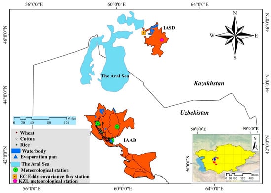
Figure 1.
Schematic diagram of the irrigation area of the Amu Darya delta (IAAD) and the irrigation area of the Syr Darya delta (IASD). National boundary data was acquired from the National Administration of Surveying, Mapping and Geoinformation with No. GS (2016) 1665.
2.2. Data Availability
Due to the long-timescale and high spatial resolution of this study, a total of 244 remote-sensing images were selected for this study, including 30 thematic mapper images (TM), 96 enhanced thematic mapper images (ETM), and 118 operational land imager images (OLI). The path/row were 159/031, 160/028, 160/030, 160/031, and 161/030. Since the year of remote sensing data needs to be consistent with other statistical data, allowing for image quality and time intervals, the years included the growing seasons (April to October) of 2000, 2005, 2012, 2015, 2019, and 2020, and the simulation results of the SEBAL model were validated in 2012 and 2019 due to limited ground measurement, and the cloud cover was less than 10%; for specific times, refer to Figure 2. The preprocessing for radiometric calibration, fast line-of-sight atmospheric analysis of spectral hypercubes (FLAASH) atmospheric correction based on a seasonal latitude surface temperature model; the brightness temperature correction and geographic correction using control points was carried out on ENVI (The Environment for Visualizing Images). In particular, the gap of ETM due to the scan line error had been filled with the striping tool in ENVI software.
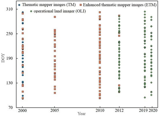
Figure 2.
Information about the acquisition time of Landsat images. (Thematic mapper images (TM), Enhanced thematic mapper images (ETM), Operational land imager (OLI)).
This study also includes meteorological station data, flux station data, digital elevation data (DEM), irrigation water data, land use and cover change data (LUCC), planting structure data, sampling point data, evaporation pan data, and yield data. In particular, the confidential data of irrigation water, planting structure and yield obtained from the Ministry of Agriculture and Water Resources (MAWR) of Uzbekistan and Ministry of MAWR of Kazakhstan were all obtained from the local field visits in 2019 and 2020 in cooperation with relevant local government departments, and have been published in a series of articles [14,15,40,44] with certain official authority. Refer to Table 1 for specific information.

Table 1.
Details of the data used in the study.
2.3. Remote Sensing Model and Data Analysis
2.3.1. SEBAL Model
The SEBAL model was initially proposed and constructed by Bastiaanssen et al. [30], to calculate the ETa; the cardinal principle was energy balance, referring to the formula below:
where Rn represents the net surface radiation flux (), is the soil heat flux (), and and represent sensible heat flux () and latent heat flux (), respectively. The respective calculations are as follows:
where and represent the surface albedo and surface emissivity. For Landsat TM/ETM/OLI images, the surface albedo (a) is calculated according to different methods [46,47,48]:
In the SEBAL model, specific emissivity mainly has two forms: thermal infrared specific emissivity (εNB) and total wide band-specific emissivity (εo). The thermal infrared specific emissivity is mainly used to calculate land surface temperature (LST). The LST and emissivity are separated from brightness temperature, and the two methods are as follows [47]:
is the short-wave solar radiation (), is the downgoing atmospheric longwave radiation (), is the longwave radiation (), represents the air density, is the air specific heat, dT represents the temperature difference between two heights (Z1 and Z2), and represents the aerodynamic resistance to heat transport. Finally, the instantaneous LET is obtained using the energy balance formula. More details on the calculation method and the “cold” and “hot” pixel selection can be found in Allen [47].
By introducing the concept of evaporation fraction (EFins), the instantaneous evapotranspiration can be extended to daily and longer periods of evapotranspiration [43,47,49,50].
represents the daily , λ stands for the latent heat of vaporization, and represent the net radiation flux and the soil heat flux over one day, and ETrF computed for the time of the image was assumed constant for the entire period represented by the image, is the representative ETrF for the period, and n is the number of days in the period. The seasonal ET was computed by summing all of the ETperiod values for the length of the season.
2.3.2. The FAO Penman–Monteith Equation
The FAO Penman–Monteith equation is considered a universal standard to estimate and is widely used around the world in the absence of measured data due to its high accuracy [51,52,53], The accuracy of SEBAL model can be verified with the FAO Penman–Monteith equation in this study. The specific formula is as follows:
where is the slope of the saturated vapor pressure curve, is the saturated vapor pressure, is the actual vapor pressure, r is the psychrometric constant, and is the wind speed at a height of 2 m. The actual evapotranspiration of crops is calculated using the Kc coefficient and the Penman–Monteith equation:
where Kc is the crop coefficient at a specific growth stage. The specific Kc value (Table 2) of wheat, rice, and maize in this study is based on the research of Schieder [54].
Table 2.
The crop coefficients of cotton, rice, and wheat.
2.3.3. Methods for Comparing Spatial Heterogeneity of ETa
Based on the least square linear regression model, the trend of evapotranspiration in this study was analyzed over the years; the specific formula is as follows:.
where i refers to the year and refers to the in the year i.
The coefficient of variation is the ratio of standard deviation to mean and can reflect the degree of variation in data from year to year [55]. The specific calculation formula is as follows:
is the annual mean value of pixels in row i and column j, is the standard deviation of pixels in row i and column j. CV is classified into four grades, which were highly stable (), stable (), unstable (), and highly unstable () (Wang et al., 2012). Combining the spatial change rate of ETa and coefficient of variation to analysis, grids with a coefficient of variation less than 0.1 (highly stable) and an ETa change rate of more than two standard deviations were defined as ‘steady drastic increase’, and grids with a coefficient of variation less than 0.1(highly stable) and an ETa change rate of less than two standard deviations were defined as ‘steady drastic reduction’ [56].
2.3.4. Validation of SEBAL Modeled ETa
The validation of ETa simulated by SEBAL model is divided into two parts: one is to verify with the measured data of the eddy covariance flux observation station (EC) and meteorological station (KZL) in the IASD and the evaporation pan in the IAAD, the other is to compare with crop evapotranspiration calculated by the FAO Penman–Monteith equation and kc. Due to the difficulty in obtaining measured data in arid inland river basins, the year of measured evapotranspiration data from flux stations and meteorological stations in the IASD is 2012, while the observed data of evaporation pan in the IAAD is 2019; the daily evapotranspiration simulated by SEBAL (ETsebal) of the corresponding data is selected for accuracy evaluation against observed evapotranspiration values (ETobserved).
2.3.5. Water Productivity
In this study, water productivity (kg/m3) was mainly divided into crop water productivity (WPc) and irrigation water productivity (WPI), which are estimated by the following equations [38]:
3. Results
3.1. Validation of the SEBAL Model
At the KZL meteorological station, the ETsebal is well-matched with the ETobserved with an R2 value of 0.86, an RMSE value of 0.85 and a percent bias of 12% (Figure 3a). This indicates that the evapotranspiration simulated by SEBAL has high precision in the oasis-agriculture area of the Aral Basin. The eddy covariance flux station shows that the SEBAL model has a slightly lower fitting degree in the desert grassland, where the R2, RMSE, and percent bias are 0.71, 0.31, and 5%, respectively (Figure 3b). For the water body, the R2, RMSE, and percent bias values between ETsebal and ETobserved are 0.81, 1.76, 15%, respectively (Figure 3c).
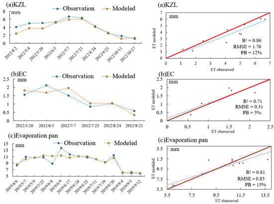
Figure 3.
Comparison of ET modeled by SEBAL (ETsebal) between ETobserved obtained from the KZL meteorological station (a), EC eddy covariance flux station (b), and evaporation pan (c).
A total of 444 crop sample sites were collected in the IAAD in 2019, including 121 rice sample points, 161 cotton sample points, and 162 wheat sample points. They were gathered around three meteorological stations in the IASD, namely Nukus, Kungrad, and Chimboy, but all lacked direct ETa observation data. The meteorological data of the corresponding SEBAL simulated date in 2019 were selected, and the crop evapotranspiration (ETc) was calculated using the Penman formula in combination with the KC coefficient, and the correlation analysis was conducted between the daily ETa value sequence of each crop sample point simulated by SEBAL and the FAO Penman–Monteith equation. The results show that 78% of the 109 cotton sampling points near the Kungard meteorological station have correlations higher than 0.6, while only 69% of the cotton samples around the Nukus meteorological station have correlations higher than 0.6 (Figure 4a). The correlation of a total of 90% of the rice sampling points around Kungrad meteorological station is higher than 0.6, with the highest value reaching 0.98. At Nukus and Chimboy meteorological stations, only 79% and 38% of the rice sampling sites have correlations higher than 0.6; there are only eight rice sampling sites near the Chimboy meteorological station; therefore, these results are more uncertain (Figure 4b). The correlation of wheat is higher overall, with all 87 wheat sampling points near Kungrad meteorological station having correlations higher than 0.6, and 93% of wheat sampling points around the Nukus meteorological station being higher than 0.6 (Figure 4c). Overall, the evapotranspiration simulated by the SEBAL model (ETsebal) has a good degree of fit with the ETc. These results demonstrate that the SEBAL model has good applicability in the study area.
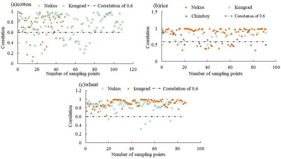
Figure 4.
The correlation analysis of ETsebal chronological sequence and ETc chronological sequence was calculated by FAO Penman–Monteith equation of all 444 crop sample sites.
3.2. The Comparison of Temporal Variations of ETa between the IAAD and the IASD
In the most recent 20 years, the trends of average evapotranspiration between the IAAD and IASD are inconsistent. Figure 5 shows the ETa inverted by SEBAL in the growing seasons (from April to October) of 2000, 2005, 2012, 2015, 2019, and 2020 in the two irrigation areas. Due to the disturbance of human activities and meteorological factors, as well as the uncertainty of SEBAL model itself, the ‘cold’ and ‘hot’ point assumption is too idealistic and long-term evapotranspiration inversion increases the uncertainty of SEBAL model results, and the maximum value of ETa in the irrigated areas fluctuates over many years. For the IAAD, the maximum value of 2087 mm for the ETa appeared in 2012 for the water body in the north of the irrigation area, while the maximum ETa in the growing season of 2020 was the smallest, being only 1676 mm. The southern part of IAAD is mostly cultivated land, while the northern part is mostly desert; therefore, ETa presents a spatial distribution pattern, high in the south and low in the north. However, the maximum value of water evaporation in the IASD appeared in 2005, reaching 1873 mm, and the maximum ETa value of 2020 was the lowest of all years surveyed, being only 1399 mm, which is consistent with the IAAD. The northern part of the IASD is mostly waterbodies, and the cultivated land and bare land are evenly distributed in space; therefore, the ETa of the IASD was higher in the north and more evenly distributed in space than that of the IAAD.
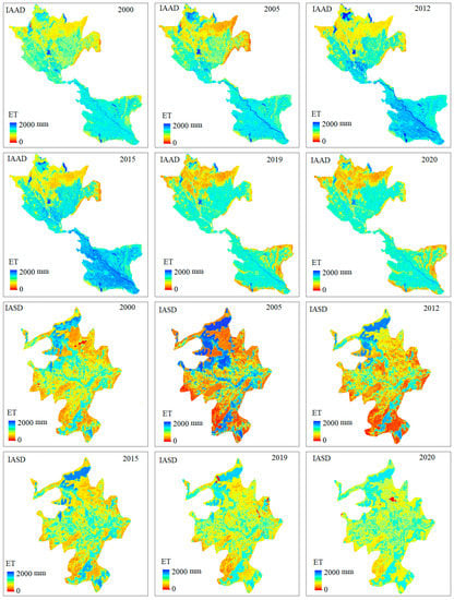
Figure 5.
The ETa was estimated by SEBAL model in the growing season from 2000 to 2020 in the irrigation of the Amu Darya delta (IAAD) and Syr Darya delta (IASD).
The monthly ETa results simulated by SEBAL from 2000 to 2020 in the IAAD and IASD are exhibited in Figure 6. The ETa of the two irrigation areas is consistent on the monthly scale and shows a single peak distribution, but is different in range. For IAAD, the average ETa in July ranged from 182 mm to 243 mm; the highest ETa was in July of 2012; and July of 2019 had the lowest ETa performance of any other month in the same period, just 182 mm. April and October are the lowest ETa months in the growing season in IAAD because of the low air temperatures and Rn, with an average ETa of only 110 mm (Figure 6a). As for IASD, the highest ETa occurred in July of 2015, reaching 198 mm, and the lowest ETa occurred in April and October, with an average of only 90mm (Figure 6b). In terms of the inter-annual scale, the ETa of the IAAD and IASD fluctuated, but the average ETa of IAAD in each year was higher than that of IASD (Figure 6c). The average ETa of IAAD over the years surveyed was 1138mm, while that of IASD was only 820 mm. In addition, the two irrigation areas had different ETa performances in the same years. For example, in 2012, IAAD had a higher ETa with an average value of 1294 mm, while IASD had a lower average ETa of just 687 mm. Furthermore, from the multi-year variation rate of ETa, the ETa of IAAD tended to decrease, whereas that of IASD tended to increase.
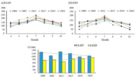
Figure 6.
(a) The average ETa performance modeled by SEBAL of each month in the growing season of 2000–2020 in the irrigation of the Amu Darya delta (IAAD), (b) in the irrigation of Syr Darya delta (IASD), and the average annual ETa comparison between the two irrigation areas (c).
3.3. The Comparison of Spatial Heterogeneity of ETa between the IAAD and IASD
The change rate of ETa in IAAD over the past 20 years was obtained using the least squares method (Figure 7a). The variation rate of ETa in the IAAD was extremely uneven in spatial distribution, whereas the change rate of ETa in the southern irrigation area was lower than the northern irrigation area. The ETa of cultivated land in the north part of the IAAD showed an obvious increasing trend, especially on the eastern and western edges of the cultivated land, which indicates that the cultivated land in the northern IAAD had a trend of outward expansion, whereas the cultivated land in the southern irrigation area was in a state of high saturation; therefore, the change rate of ETa was low, maintaining a low rate of growth even at the edge of the cultivated land, as ETa tended to decrease due to abandoned farming. As a result of a reduction in the area of wetland and natural vegetation coverage, the ETa of some wetlands in the north of IAAD tended to decrease. The change rate of the ETa of the waterbody in the IAAD was not large, fluctuating around 0. Due to the factors of abandoned farming and cultivated land expansion, the change rate of the ETa of the cultivated land in the IASD increased and decreased locally (Figure 7b). On the whole, the cultivated land expansion trend is obvious. Similarly, due to the reduction in wetland area and natural vegetation area, the ETa of wetland in IASD showed a significant trend of reduction, whereas the change rate of the waterbody in the IASD was not obvious, also fluctuating around 0. The coefficient of variation of the IAAD is shown in Figure 7c, where it can be seen that the regions with a greater coefficient of variation in ETa mostly occur in the regions with changes in land-use types. The ETa stability of cultivated land area in IAAD was higher, and the ETa stability of the waterbody was also higher, whereas the ETa stability of the cultivated land edge and wetland was lower due to the drastic changes in the area. The ETa instability in the IASD was 46% less than the IAAD due to more potential arable land for development, which will lead to an increase in ETa in the future (Figure 7d); the change in the cultivated land area led to the instability of ETa. Similarly, the stability of wetlands in the IASD was low, whereas the stability of the waterbody was high.
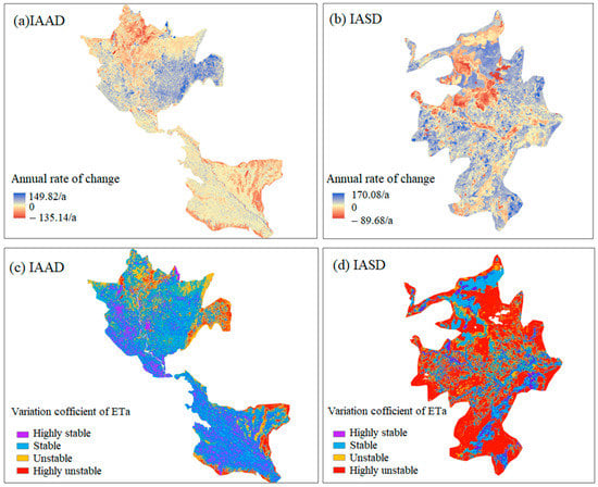
Figure 7.
(a) Multi-year spatial variation rate of ETa of the irrigation of Amu Darya delta (IAAD) and (b) the irrigation of Syr Darya delta (IASD), the variation coefficient of ETa of the IAAD (c), and the IASD (d).
Due to the reduction in wetland area, there were plots with a steady drastic reduction in ETa in the IAAD that cover an area of 412 km2. At the same time, there were obvious expansions of cultivated land in the northern IAAD, leading to stable and drastic increases in ETa at some edges of cultivated land with an area of 937 km2. As for the IASD, the regions where ETa was stable or drastically reduced were mainly located in wetland areas of up to 165 km2. Although the IASD has more potential farmland, its reclamation intensity and irrigation efficiency were lower than in the IAAD; therefore, there was no dramatic increase in evapotranspiration in the irrigation area.
In conclusion, the stability of ETa in the IAAD was higher than in the IASD due to currently small potential cultivated land area, but due to the higher irrigation water supply and lower water productivity, which will be discussed below, the change rate of ETa in the IAAD was much higher than IASD locally.
3.4. The Comparison of Water Productivity between the IAAD and IASD
Based on the detailed LUCC classification map in 2019 and combined with the inversion ETa, the water productivity of the main crop types in the two irrigated areas was compared. Figure 8a,b shows the main crop area in the two irrigation areas; wheat is the dominant crop in the IAAD, whereas the IASD is mainly cultivated with cotton. By comparing the ETa of the main crop types in the two irrigation areas, it can be seen that the average ETa of cotton, rice, orchards, and vegetables in the IAAD is higher than that in IASD. Wheat is the only exception. Among all crops, rice and orchards have the highest ETa, followed by cotton and wheat, and vegetables have the lowest (Figure 8c). In addition, the area of all crops in the IASD is much smaller than that in IAAD, which also explains why the ETa of the IASD is much smaller than that of the IAAD (Figure 8d,e).
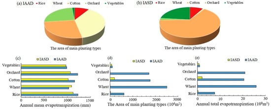
Figure 8.
(a) The main crop type proportions in the irrigation of Amu Darya delta (IAAD), (b) The main crop type proportions in the irrigation of Syr Darya delta (IASD), (c) ETa of main crop types in two irrigation areas, (d) The area of main crop types, and (e) annual total ETa among main crop types.
As shown in Figure 9a, the irrigation water supply in the IAAD is much higher than that in the IASD. More specifically, there are obvious dry and wet years in the IAAD; in 2005, there was a large amount of irrigation water, but in years with more cultivated land, such as in 2000, there was little water for irrigation. The uneven distribution and unreasonable allocation of water resources in time and space in the IAAD cause more water waste. Combined with the statistical data on crop yield, the WPc and WPI of wheat, rice, and cotton in the two irrigated areas have been calculated. The average WPc of cotton in the IASD (cotton—S) is 0.19 kg/m3, whereas in the IAAD (cotton—A) it is 0.17 kg/m3, the average WPc for wheat (wheat—S) is 0.42 kg/m3, and wheat—N is 0.32 kg/m3; rice WPc averages 0.40 kg/m3 (rice—S), and just 0.27 kg/m3 in IAAD. In general, the WPc of each crop in the IASD is higher than that in the IAAD; this reflects the fact that Kazakhstan’s irrigation system and technology are superior to Uzbekistan’s (Figure 9b,c).
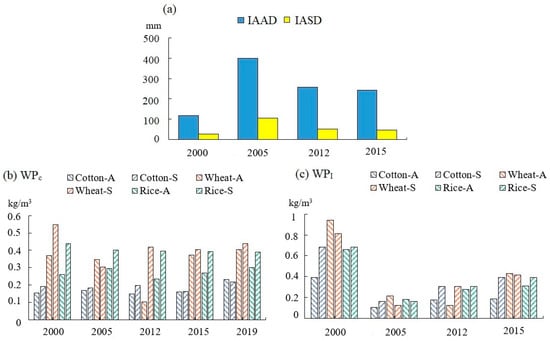
Figure 9.
(a) The irrigation water supply in irrigation of Amu Darya delta (IAAD) and Syr Darya delta (IASD), (b) the crop water productivity (WPc) on the IAAD and IASD, (c) the irrigation water productivity (WPI) on the IAAD and IASD. the suffix-A stands for IAAD and the suffix-S stands for IASD.
4. Discussion
4.1. Accuracy Assessment of the SEBAL Model
In this study, the ETa modeled by SEBAL in the IAAD is between 900 mm and 1200 mm from 2000 to 2020, whereas the ETa of IASD is between 600 mm and 900 mm. Compared with the measured data of meteorological station, flux station, and evaporation pan in the study area, the SEBAL-modeled ETa fits the measured data well, with R2 higher than 0.7, maximum RMSE at 1.76, and maximum percent bias at 15%. However, due to the large area, complex land-cover types, and scarcity of measured points, it is far from enough to evaluate the SEBAL simulation results with only a few measured data point. Therefore, the Penman–Monteith equation is also used to verify the modeled results. The ETc calculated by the Penman–Monteith equation and the crop coefficient Kc is also used to verify the modeled results. The results show that the SEBAL model has a good simulation result for the ETc of crops: the average R2 of rice was 0.84 and percent bias was 7.02%, the average R2 and a percent bias of wheat were 0.80 and 7.23%, and the average R2 and a percent bias of cotton were 0.72 and 10.89%. Because the water content of rice is more abundant, close to the optimal soil moisture conditions described in ETo, the correlation between ETc and ETa of rice is higher than wheat and cotton. The ETa returned by this study still needs to be compared with that in previous studies.
Ochege et al. [43] simulated the ETa of the IASD in 2012 using the SEBAL model, and the results showed that the growing season ETa for land surfaces ranged between 658 and 850 mm; the average ETa of the IASD was 687 mm and the average ETa of cultivated land was 842 mm. Conrad et al. [42] used the SEBAL model to invert the ETa in the south IAAD in 2004. The seasonal ETa was over 1200 mm from April to October, and the ETa modeled in IAAD for 2005 was 1294 mm. Liu et al. [14] also used the SEBAL model to invert the ETa in the north IAAD over the past 30 years and found that the ETa ranged from 900 mm to 1200 mm, which is consistent with this study. Besides remote sensing inversion research, the evaporation from oasis agriculture could be as high as 1546 mm in central Asia [57]; the observed ETa of the Aral Sea in 1990 reached 1220 mm [58]. Using the water balance to calculate the evapotranspiration of the Aral Sea from 1911 to 1989, the annual evapotranspiration of the Aral Sea was between 900 mm and 1100 mm [3], and combined with a mathematical method to predict the evaporation of the Aral Sea from 2000 to 2050 with an average annual increase of 1.5 m, it could reach 1500 mm [59]. To sum up, the simulation ETa results of this study are comparable to previous studies, which proves the applicability of the SEBAL model to typical irrigation areas of the Aral Sea basin.
4.2. The Impact of LUCC on ETa Variations
For nearly 20 years, temperatures in both IAAD and IASD have fluctuated around 12.5 °C. However, the ETa of the IAAD is quite different from IASD in terms of temporal and spatial variation. Because ESA’s LUCC data are relatively robust in identifying land cover temporal changes [60], they are used for analysis in order to explain the following differences. However, the resolution of LUCC data is 300 m, whereas the resolution of ETa inversed by SEBAL is 30 m, indicating a mismatch in scale and increasing the deviation of ETa among kinds of land use.
- The average ETa of IAAD is much higher than that of IASD. Figure 10a shows the ETa of different land covers from 2000 to 2015; there is no significant difference in the waterbodies or the woodland, whereas there is a large difference in the cultivated land. The ETa of cultivated land in IAAD is maintained at over 1150 mm for many years due to higher irrigation and lower water productivity, as discussed below, whereas that of IASD is around 800 mm. Considering the proportion of cultivated land in the two irrigation areas (Figure 10b,c), it can be concluded that the variation of cultivated land is the main reason for the spatio-temporal heterogeneity of ETa. The IASD is largely distributed between cultivated and bare land, leading to a much lower ETa than for the IAAD, which is mainly composed of cultivated land.
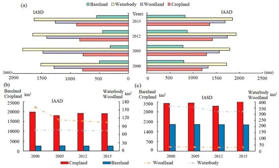 Figure 10. (a) ETa of main landcover types in two irrigation areas, (b) the changes of main landcover area in the Amu Darya delta (IAAD), (c) the changes of main landcover area in the Syr Darya delta (IASD).
 - In the past 20 years, the ETa of IAAD showed a decreasing trend, whereas that of IASD showed an increasing trend. The cultivated land area in the IAAD decreased from 1992 to 2005 and increased from 2010 to 2015; there is a decreasing trend on the whole, which is consistent with the previous research [14,61,62]. As a result, the ETa has tended to decrease. The cultivated area of the IASD has shown a slightly increasing trend during the past 20 years, accompanied by an increasing ETa.
- The stability of ETa in the IAAD is higher than that of the IASD. It is precisely because of the low saturation of the cultivated land in the IASD that the ETa instability in the irrigation area has increased. The cultivated land of IASD accounts for 60% of the total irrigation area, and there is still a large amount of arable land for development. The cultivated land area of IASD has shown an increasing trend recently. From 2012 to 2015, the cultivated land area of IASD has increased by 100 km2; the ETa of the IASD also showed an increasing trend (Figure 6c), which directly leads to the instability of the IASD’S ETa. In the IAAD, the cultivated land accounts for 87% of the total area, and the cultivated land area tends to be saturated; therefore, the stability of ETa is relatively high.
4.3. Accuracy Assessment of Water Productivity and Policy Implications
The WPc and WPI of IAAD are lower than that of IASD because the average irrigation water consumption of IAAD during 2000, 2005, 2012, and 2015 is 4.18 times than IASD, and the ETa of the IAAD is 1.38 times than IASD over the same period. The ETa of irrigation areas is affected by LUCC to a certain extent [55] and by the irrigation amount, together affecting the regional water productivity (WPc and WPI). Meanwhile, there are some deviations in the statistical survey methods of different countries, which also bring uncertainty to the assessment of water productivity.
Compared with previous studies, the water productivity in this study is lower than the field observations but close to the remote sensing results, which is consistent with Liu et al.’s [40] conclusion, who calculated that the average results of grain WPc in Central Asia from 2000 to 2016 were 0.24–0.39 kg/m3, and 0.21–0.27 kg/m3 for cotton. Using an SSEB remote sensing model, the WPc of cotton in the typical irrigation area of the Syr River basin in 2006 was calculated as reaching 0–0.54 kg/m3 [41]. The site observations of cotton WPc in the Syr River basin and Fergana basin were 0.40–0.75 kg/m3 and 0.38–0.89 kg/m3 [63,64]. The grain and cotton WPc of the Aral Sea basin from 2000 to 2014 were 0.88 and 0.45, respectively, according to WUEMoCA statistics [10]. This study also confirmed that crop and water productivity in irrigated areas along the Syr Darya river was greater than the Amu Darya River. Except for wheat, the WPI of other crop types in the IAAD was lower than in the IASD, findings which are in line with those of Liu et al. [40]. These can be compared with the WPc of other regions: maize WPc values average 2.1 kg/m3 at the Agricultural Science Center at Farmington [65], the WPc of grain in the Heihe basin in China is 0.83 kg/m3 [66], and the maize WPc in India is 1.58 kg/m3 [67]. The crop water productivity around the Aral Sea basin has a huge potential to increase.
There are some ways to improve crop water productivity and reduce evapotranspiration, including policies, regulations, and technology. After the collapse of the Soviet Union, land reform in Kazakhstan and Uzbekistan differed in intensity. Kazakhstan’s land reform model was relatively radical, and privatization of agricultural land was carried out. However, Uzbekistan has not fully implemented privatization; inadequate irrigation systems and infrastructure make Uzbekistan extremely inefficient in terms of water productivity. One direction of agricultural policy adjustment in the future still lies in promoting the development of farms, reforming support service systems, and strengthening infrastructure construction.
The agricultural irrigation water in the arid regions of Central Asia is largely dependent on irrigation canals and drainage networks. Under this irrigation mode, the water consumption of non-productive evapotranspiration, such as in a canal system, dissipates greatly. Fully utilizing the water from rainfall and reducing the irrigation water can help obtain the greatest WPc [68]; meanwhile, adopting new irrigation and crop management strategies can improve water productivity. Irmak et al. [69] demonstrated that 75% of the full irrigation treatment, with no yield penalty under subsurface drip and sprinkler irrigation, can save 25% of irrigation water. In terms of economic efficiency per efficiency of water quantity in water use, Lee and Jung [70] suggested converting wheat into cotton using drip irrigation, whose efficiency was the highest. Furthermore, combining this with the agriculture model [71] and remote-sensing data can provide information about the cultivated land area, pests, land productivity, etc., for agricultural production. Guided by this information, appropriate irrigation systems and policies can be developed to ensure that unnecessary water consumption is reduced while maintaining the crop yield. To sum up, countries in the Aral Sea basin still need to make efforts to improve water productivity, maintain the Aral Sea area, and reduce unnecessary water resource waste.
5. Conclusions
This study used the SEBAL model to simulate ETa in two main irrigation areas around the Aral Sea from 2000 to 2020, and calculated water productivity to compare and analyze water consumption and water productivity in the two irrigation areas. The ETa simulated by the SEBAL model matched the crop evapotranspiration (ETc) calculated by the Penman–Monteith method, with a correlation coefficient higher than 0.8. The correlation coefficient between the SEBAL modeled ETa and the ET observed at meteorological stations, the Eddy Covariance Flux Station data, and evaporation pan measured data were 0.86, 0.71, and 0.81, respectively. The results show that the average annual ETa of the IAAD was 1138 mm, whereas that of the IASD was 687 mm. The reasons for this difference are that the IAAD has a higher cultivated land area, higher irrigation water supply, and lower water productivity. However, there was a large amount of developable cultivated land in the IASD; therefore, the annual ETa has shown an increasing trend with low stability. In the IAAD, where the phenomenon of abandoned arable land was serious, the ETa showed a decreasing trend with high stability. The amount of irrigation water in the IAAD fluctuated greatly, being near m3 higher than that in the IASD in the same period. Meanwhile, the water productivity of IAAD was lower than IASD, which reflects Uzbekistan and Kazakhstan’s differences in water productivity, to a certain extent. However, there is a long process for improvement in water productivity for IAAD and IASD, which can be achieved by reducing non-productive evapotranspiration and adopting new irrigation and crop management strategies such as subsurface drip and sprinkler irrigation.
This study verifies the reliability of energy balance models such as the SEBAL model in ET inversion in the Aral Sea basin, and also provides ideas for ET inversion in arid regions with little data; it also provides reference data for agricultural water management and water resource protection in the Aral Sea basin.
Author Contributions
Conceptualization, Z.L. and T.L.; methodology, Z.L.; software, Z.L.; validation, Z.L.; formal analysis, Y.H.; investigation, Z.L.; resources, T.L.; data curation, Z.L., Y.D., X.P., and W.W.; writing—original draft preparation, Z.L.; writing—review and editing, Z.L.; visualization, Z.L.; supervision, Z.L.; project administration, T.L.; funding acquisition, T.L. All authors have read and agreed to the published version of the manuscript.
Funding
This research was funded by the Strategic Priority Research Program of the Chinese Academy of Sciences, Pan-Third Pole Environment Study for a Green Silk Road (Grant No. XDA20060301), the National Natural Science Foundation of China (Grant No. 42071245), the International Partnership Program of the Chinese Academy of Sciences (Grant No. 131551KYS B20160002), K.C.Wong Education Foundation (GJTD-2020-1), CAS Interdisplinary Innovation Team (Grant No. JCTD-2019-20) and Talent start-up fee (Grant No. 2021r020).
Institutional Review Board Statement
Not applicable.
Informed Consent Statement
Not applicable.
Data Availability Statement
The data presented in this study are available on request from the corresponding author.
Conflicts of Interest
The authors declare that they have no known competing financial interest or personal relationships that could have appeared to influence the work reported in this paper.
References
- Boomer, I.; Aladin, H.; Plotnikov, I.; Whatley, R. The palaeolimnology of the Aral Sea: A review. Quat. Sci. Rev. 2000, 19, 1259–1278. [Google Scholar] [CrossRef]
- Philip, M. The future Aral Sea: Hope and despair. Environ. Earth Sci. 2016, 75, 844. [Google Scholar]
- Bortnik, V.N. Changes in the water-level and hydrological balance of the Aral Sea. In The Aral Sea Basin; Springer: Berlin/Heidelberg, Germany, 1996; pp. 25–32. [Google Scholar]
- Su, Y.; Li, X.; Feng, M.; Nian, Y.; Huang, L.; Xie, T.; Zhang, K.; Chen, F.; Huang, W.; Chen, J.; et al. High agricultural water consumption led to the continued shrinkage of the Aral Sea during 1992–2015. Sci. Total Environ. 2021, 777, 145993. [Google Scholar] [CrossRef]
- Su, Y.Y.; Li, Y.P.; Liu, Y.R.; Fan, Y.R.; Gao, P.P. Development of an integrated PCA-SCA-ANOVA framework for assessing multi-factor effects on water flow: A case study of the Aral Sea. CATENA 2021, 197, 104954. [Google Scholar] [CrossRef]
- Li, Q.; Li, X.; Ran, Y.; Feng, M.; Nian, Y.; Tan, M.; Chen, X. Investigate the relationships between the Aral Sea shrinkage and the expansion of cropland and reservoir in its drainage basins between 2000 and 2020. Int. J. Digit. Earth 2020, 14, 661–677. [Google Scholar] [CrossRef]
- Gaybullaev, B.; Chen, S.C.; Kuo, Y.M. Large-scale desiccation of the Aral Sea due to over-exploitation after 1960. J. Mt. Sci. 2012, 9, 538–546. [Google Scholar] [CrossRef]
- Aladin, N.V.; Hoeg, J.T.; Plotnikov, I. Small Aral Sea brings hope for Lake Balkhash. Science 2020, 370, 1283. [Google Scholar] [CrossRef] [PubMed]
- Asarin, A.E.; Kravtsova, V.I.; Mikhailov, V.N. Amudarya and Syrdarya Rivers and Their Deltas; Springer: Berlin/Heidelberg, Germany, 2009. [Google Scholar]
- Zhang, J.; Chen, Y.; Li, Z.; Song, J.; Fang, G.; Li, Y.; Zhang, Q. Study on the utilization efficiency of land and water resources in the Aral Sea Basin, Central Asia. Sustain. Cities Soc. 2019, 51, 101693. [Google Scholar] [CrossRef]
- Assiya, M.; Jilili, A.; Sanim, B.; Botagoz, I.; Zhassulan, S. Water balance of the Small Aral Sea. Environ. Earth Sci. 2020, 79, 75. [Google Scholar]
- Jarsjo, J.; Destouni, G. Groundwater discharge into the Aral Sea after 1960. J. Marine Syst. 2004, 47, 109–120. [Google Scholar] [CrossRef]
- Schettler, G.; Oberhänsli, H.; Stulina, G.; Djumanov, J.H. Hydrochemical water evolution in the Aral Sea Basin. Part II: Confined groundwater of the Amu Darya Delta Evolution from the headwaters to the delta and SiO2 geothermometry. J. Hydrol. 2013, 495, 285–303. [Google Scholar] [CrossRef]
- Liu, Z.; Huang, Y.; Liu, T.; Li, J.; Xing, W.; Akmalov, S.; Peng, J.; Pan, X.; Guo, C.; Duan, Y. Water Balance Analysis Based on a Quantitative Evapotranspiration Inversion in the Nukus Irrigation Area, Lower Amu River Basin. Remote Sens. 2020, 12, 2317. [Google Scholar] [CrossRef]
- Pan, X.; Wang, W.; Liu, T.; Huang, Y.; De Maeyer, P.; Guo, C.; Ling, Y.; Akmalov, S. Quantitative Detection and Attribution of Groundwater Level Variations in the Amu Darya Delta. Water 2020, 12, 2869. [Google Scholar] [CrossRef]
- Pocas, I.; Calera, A.; Campos, I.; Cunha, M. Remote sensing for estimating and mapping single and basal crop coefficientes: A review on spectral vegetation indices approaches. Agric. Water Manag. 2020, 233, 106081. [Google Scholar] [CrossRef]
- Leuning, R.; Sands, P. Theory and practice of a portable photosynthesis instrument. Plant Cell Environ. 1989, 12, 669–678. [Google Scholar] [CrossRef]
- Kizer, M.A.; Elliott, R.L. Eddy correlation systems for measuring evaporatranspiration. Trans. ASAE 1991, 34, 387–392. [Google Scholar] [CrossRef]
- Wright, J.L. Using weighing lysimeters to develop evapotranspiration Crop Coefficients. In Lysimeters for Evapotranspiration & Environmental Measurements; ASCE: Reston, VA, USA, 1991. [Google Scholar]
- Nagler, P.L.; Scott, R.L.; Westenburg, C.; Cleverly, J.R.; Glenn, E.P.; Huete, A.R. Evapotranspiration on western US rivers estimated using the Enhanced Vegetation Index from MODIS and data from eddy covariance and Bowen ratio flux towers. Remote Sens. Environ. 2005, 97, 337–351. [Google Scholar] [CrossRef]
- Xiang, K.; Li, Y.; Horton, R.; Feng, H. Similarity and difference of potential evapotranspiration and reference crop evapotranspiration—A review. Agric. Water Manag. 2020, 232, 106043. [Google Scholar] [CrossRef]
- Crétaux, J.F.; Kouraev, A.V.; Papa, F.; Bergé-Nguyen, M.; Cazenave, A.; Aladin, N.; Plotnikov, I.S. Evolution of sea level of the big Aral Sea from satellite altimetry and its implications for water balance. J. Great Lakes Res. 2005, 31, 520–534. [Google Scholar] [CrossRef] [Green Version]
- Sing, A.; Behrangi, A.; Fisher, J.B.; Reager, J.T. On the Desiccation of the South Aral Sea Observed from Spaceborne Missions. Remote Sens. 2018, 10, 793. [Google Scholar] [CrossRef] [Green Version]
- Miralles, D.G.; Holmes, T.R.H.; De Jeu, R.A.M.; Gash, J.H.; Meesters, A.G.C.A.; Dolman, A.J. Global land-surface evaporation estimated from satellite-based observations. Hydrol. Earth Syst. Sci. 2011, 15, 453–469. [Google Scholar] [CrossRef] [Green Version]
- Khan, M.S.; Liaqat, U.W.; Baik, J.; Choi, M. Stand-alone uncertainty characterization of GLEAM, GLDAS and MOD16 evapotranspiration products using an extended triple collocation approach. Agric. For. Meteorol. 2018, 252, 256–268. [Google Scholar] [CrossRef]
- Martens, B.; De Jeu, R.A.M.; Verhoest, N.E.C.; Schuurmans, H.; Kleijer, J.; Miralles, D.G. Towards Estimating Land Evaporation at Field Scales Using GLEAM. Remote Sens. 2018, 10, 1720. [Google Scholar] [CrossRef] [Green Version]
- Fisher, J.B.; Lee, B.; Purdy, A.J.; Halverson, G.H.; Dohlen, M.B.; Cawse-Nicholson, K.; Wang, A.; Anderson, R.G.; Aragon, B.; Arain, M.A.; et al. Ecostress: Nasa’s Next-Generation Mission to Measure Evapotranspiration from the International Space Station. Water Resour. Res. 2020, 56, e2019WR026058. [Google Scholar] [CrossRef]
- Aragon, B.; Ziliani, M.G.; Houborg, R.; Franz, T.E.; McCabe, M.F. CubeSats deliver new insights into agricultural water use at daily and 3 m resolutions. Sci. Rep. 2021, 11, 12131. [Google Scholar] [CrossRef]
- Norman, J.M.; Kustas, W.P.; Humes, K.S. Source approach for estimating soil and vegetation energy fluxes in observations of directional radiometric surface temperature. Agric. For. Meteorol. 1995, 77, 263–293. [Google Scholar] [CrossRef]
- Bastiaanssen, W.G.M.; Menenti, M.; Feddes, R.A.; Holtslag, A.A.M. A remote sensing surface energy balance algorithm for land (SEBAL)-1. Formulation. J. Hydrol. 1998, 212, 198–212. [Google Scholar] [CrossRef]
- Su, Z. The Surface Energy Balance System (SEBS) for estimation of turbulent heat fluxes. Hydrol. Earth Syst. Sci. 2002, 6, 85–100. [Google Scholar] [CrossRef]
- Allen, R.G.; Tasumi, M.; Trezza, R. Satellite-based energy balance for mapping evapotranspiration with internalized calibration (METRIC)—Model. J. Irrig. Drain. Eng. 2007, 133, 380–394. [Google Scholar] [CrossRef]
- Majozi, N.P.; Mannaerts, C.M.; Ramoelo, A.; Mathieu, R.; Mudau, A.E.; Verhoef, W. An intercomparison of satellite-based daily evapotranspiration estimates under different eco-climatic regions in South Africa. Remote Sens. 2017, 9, 307. [Google Scholar] [CrossRef] [Green Version]
- Jamshidi, S.; Zand-parsa, S.; Pakparvar, M.; Niyogi, D. Evaluation of evapotranspiration over a semiarid region using multiresolution data sources. J. Hydrometeorol. 2019, 20, 947–964. [Google Scholar] [CrossRef]
- Jamshidi, S.; Zand-Parsa, S.; Naghdyzadegan Jahromi, M.; Niyogi, D. Application of a simple Landsat-MODIS fusion model to estimate evapotranspiration over a heterogeneous sparse vegetation region. Remote Sens. 2019, 11, 741. [Google Scholar] [CrossRef] [Green Version]
- Acharya, B.; Sharma, V. Comparison of Satellite Driven Surface Energy Balance Models in Estimating Crop Evapotranspiration in Semi-Arid to Arid Inter-Mountain Region. Remote Sens. 2021, 13, 1822. [Google Scholar] [CrossRef]
- Niyogi, D.; Sajad, J.; David, S.; Olivia, K. Evapotranspiration climatology of indiana using in situ and remotely sensed products. J. Appl. Meteorol. Climatol. 2020, 59, 2093–2111. [Google Scholar] [CrossRef]
- Fernández, J.E.; Alcon, F.; Diaz-Espejo, A.; Hernandez-Santana, V.; Cuevas, M.V. Water use indicators and economic analysis for on-farm irrigation decision: A case study of a super high density olive tree orchard. Agric. Water Manag. 2000, 237, 106–123. [Google Scholar] [CrossRef]
- Zeri, M.; Hussain, M.Z.; Anderson-Teixeira, K.J.; DeLucia, E.; Bernacchi, C.J. Water use efficiency of perennial and annual bioenergy crops in central Illinois. J. Geophys. Res.-Biogeosci. 2013, 118, 581–589. [Google Scholar] [CrossRef] [Green Version]
- Liu, S.; Luo, G.; Wang, H. Temporal and Spatial Changes in Crop Water Use Efficiency in Central Asia from 1960 to 2016. Sustainability 2020, 12, 572. [Google Scholar] [CrossRef] [Green Version]
- Platonov, A.; Thenkabail, P.S.; Biradar, C.M.; Cai, X.; Gumma, M.; Dheeravath, V.; Cohen, Y.; Alchanatis, V.; Goldshlager, N.; Ben-Dor, E.; et al. Water Productivity Mapping (WPM) Using Landsat ETM plus Data for the Irrigated Croplands of the Syrdarya River Basin in Central Asia. Sensors 2008, 8, 8156–8180. [Google Scholar] [CrossRef] [Green Version]
- Conrad, C.; Dech, S.W.; Hafeez, M.; Lamers, J.; Martius, C.; Strunz, G. Mapping and assessing water use in a Central Asian irrigation system by utilizing MODIS remote sensing products. Irrig. Drain. Syst. 2007, 21, 218. [Google Scholar] [CrossRef] [Green Version]
- Ochege, F.U.; Luo, G.P.; Obeta, M.C.; Owusu, G.; Duulatov, E.; Cao, L.Z.; Nsengiyumva, J.B. Mapping evapotranspiration variability over a complex oasis-desert ecosystem based on automated calibration of Landsat 7 ETM+ data in SEBAL. GISci. Remote Sens. 2019, 28, 1305–1332. [Google Scholar] [CrossRef]
- Khaydar, D.; Chen, X.; Huang, Y.; Ilkhom, M.; Liu, T.; Friday, O.; Farkhod, A.; Khusen, G.; Gulkaiyr, O. Investigation of crop evapotranspiration and irrigation water requirement in the lower Amu Darya River Basin, Central Asia. J. Arid. Land. 2021, 13, 23–39. [Google Scholar] [CrossRef]
- Liu, T. A Dataset of Planting Structure in the Aral Sea Basin (2019); National Tibetan Plateau Data Center: Beijing, China, 2021. [Google Scholar]
- Liang, S.L. Narrowband to broadband conversions of land surface albedo I Algorithms. Remote Sens. Environ. 2001, 76, 213–238. [Google Scholar] [CrossRef]
- Allen, R.; Tasumi, M.; Trezza, R.; Bastiaanssen, W. SEBAL (Surface Energy Balance Algorithms for Land)-Advanced Training and User’s Manual-Idaho Implementation, Version 1.0; WaterWatch, Inc.: Wageningen, The Netherlands, 2002; pp. 1–98. [Google Scholar]
- Hanqiu, X. Retrieval of the reflectance and land surface temperature of the newly-launched landsat 8 satellite. Chin. J. Geophys. Chin. Ed. 2015, 58, 741–747. [Google Scholar]
- Al Zayed, I.S.; Elagib, N.A.; Ribbe, L.; Heinrich, J. Satellite-based evapotranspiration over Gezira Irrigation Scheme, Sudan: A comparative study. Agric. Water Manag. 2016, 177, 66–76. [Google Scholar] [CrossRef]
- Cuenca, R.H.; Ciotti, S.P.; Hagimoto, Y. Application of Landsat to Evaluate Effects of Irrigation Forbearance. Remote Sens. 2013, 5, 3776–3802. [Google Scholar] [CrossRef] [Green Version]
- Sentelhas, P.C.; Gillespie, T.J.; Santos, E.A. Evaluation of FAO Penman–Monteith and alternative methods for estimating reference evapotranspiration with missing data in Southern Ontario, Canada. Agric. Water Manag. 2010, 97, 644. [Google Scholar] [CrossRef]
- Bala, A.; Rawat, K.S.; Misra, A.K.; Srivastava, A. Assessment and validation of evapotranspiration using SEBAL algorithm and Lysimeter data of IARI agricultural farm, India. Geocarto Int. 2016, 31, 739–764. [Google Scholar] [CrossRef]
- Rahimzadegan, M.; Janani, A. Estimating evapotranspiration of pistachio crop based on SEBAL algorithm using Landsat 8 satellite imagery. Agric. Water Manag. 2019, 217, 383–390. [Google Scholar] [CrossRef]
- Schieder, T.M. Analysis of water use and allocation for the Khorezm region in Uzbekistan using an integrated economic-hydrological mode. Phys. Status Solidi. 2011, 86, 671–678. [Google Scholar]
- Whelen, T.; Siqueira, P. Coefficient of variation for use in crop area classification across multiple climates. Int. J. Appl. Earth Obs. 2018, 67, 114–122. [Google Scholar] [CrossRef]
- Wang, Y.F.; Shen, Y.J.; Chen, Y.N.; Guo, Y. Vegetation dynamics and their response to hydroclimatic factors in the Tarim River Basin, China. Ecohydrology 2012, 6, 927–936. [Google Scholar] [CrossRef]
- Li, L.; Luo, G.; Chen, X.; Li, Y.; Xu, G.; Xu, H.; Bai, J. Modelling evapotranspiration in a Central Asian desert ecosystem. Ecol. Model. 2011, 222, 3691. [Google Scholar] [CrossRef]
- Small, E.E.; Sloan, L.C.; Hostetler, S.; Giorgi, F. Simulating the water balance of the Aral Sea with a coupled regional climate-lake model. J. Geophys. Res. 1999, 104, 6583. [Google Scholar] [CrossRef]
- Létolle, R.; Aladin, N.; Filipov, I.; Boroffka, N. The future chemical evolution of the Aral Sea from 2000 to the years 2050. Mitig. Adapt. Strateg. Glob. Chang. 2005, 10, 51–70. [Google Scholar] [CrossRef]
- Bicheron, P.; Huc, M.; Henry, C.; Bontemps, S.; Lacaux, J.P. GlobCover Products Description Manual; European Space Agency (ESA): Paris, France, 2008; p. 25. [Google Scholar]
- Rakhmatullaev, S.; Huneau, F.; Celle-Jeanton, H.; Le Coustumer, P.; Motelica-Heino, M.; Bakiev, M. Water reservoirs, irrigation and sedimentation in Central Asia: A first-cut assessment for Uzbekistan. Environ. Earth Sci. 2013, 68, 998. [Google Scholar] [CrossRef] [Green Version]
- Li, J. The Impact of Climate Change on Natural Resources in Central Asian; China Meteorological Press: Beijing, China, 2017. [Google Scholar]
- Abdullaev, I.; Molden, D. Spatial and temporal variability of water productivity in the Syr Darya Basin, central Asia. Water Resour. Res. 2004, 40, 2364. [Google Scholar] [CrossRef]
- Reddy, J.M.; Muhammedjanov, S.; Jumaboev, K.; Eshmuratov, D. Analysis of Cotton Water Productivity in Ferghana Valley of Central Asia. Agric. Sci. 2012, 3, 822–834. [Google Scholar]
- Djaman, K.; O’Neill, M.; Owen, C.K.; Smeal, D.; Koudahe, K. Crop Evapotranspiration, Irrigation Water Requirement and Water Productivity of Maize from Meteorological Data under Semiarid Climate. Water 2018, 10, 405. [Google Scholar] [CrossRef] [Green Version]
- Tan, M.; Zheng, L. Increase in economic efficiency of water use caused by crop structure adjustment in arid areas. J. Environ. Manag. 2019, 230, 386–391. [Google Scholar] [CrossRef]
- Mishra, H.S.; Rathore, T.R.; Savita, U.S. Water-use efficiency of irrigated winter maize under cool weather conditions of India. Irrig. Sci. 2001, 21, 27–33. [Google Scholar]
- Howell, T.A. Enhancing water use efficiency in irrigated agriculture. Agron. J. 2001, 93, 281–289. [Google Scholar] [CrossRef] [Green Version]
- Irmak, S.; Djaman, K.; Rudnick, D.R. Effect of full and limited irrigation amount and frequency on subsurface drip-irrigated maize evapotranspiration, yield, water use efficiency and yield response factors. Irrig. Sci. 2016, 34, 271–286. [Google Scholar] [CrossRef]
- Lee, S.O.; Jung, Y. Efficiency of water use and its implications for a water-food nexus in the Aral Sea Basin. Agric. Water Manag. 2018, 207, 80–90. [Google Scholar] [CrossRef]
- Nkomozepi, T.; Chung, S.O. Assessing the trends and uncertainty of maize net irrigation water requirement estimated from climate change projections for Zimbabwe. Agric. Water Manag. 2012, 111, 60–67. [Google Scholar] [CrossRef]


Publisher’s Note: MDPI stays neutral with regard to jurisdictional claims in published maps and institutional affiliations. |
© 2022 by the authors. Licensee MDPI, Basel, Switzerland. This article is an open access article distributed under the terms and conditions of the Creative Commons Attribution (CC BY) license (https://creativecommons.org/licenses/by/4.0/).