Research on the Measurement Accuracy of Shipborne Rayleigh Scattering Lidar

Abstract

This paper aims to study the measurement accuracy of Rayleigh scattering lidar (light detection and ranging) based on a ship platform and analyze the influence of the laser beam uncertainty on the temperature inversion results. Taking the ship platform roll data as a reference, the Rayleigh scattering lidar oscillating model is simplified to a sine function, and the inversion accuracy of atmospheric temperature is analyzed under different settled observation angles and different roll angles. When the settled observation angle is 0° and the roll angle amplitudes are 10°, 20°, and 30°, the maximum deviations of the temperature within the height range of 30–80 km are 3.47 K, 13.73 K, and 22.78 K, respectively, and the average deviations are 2.35 K, 9.09 K, and 12.95 K, respectively. When the observation angle is set to 30° and the roll angle amplitudes are 10°, 20°, and 30°, the maximum deviations of the temperature within the height range of 30–80 km are 11.75 K, 27.49 K, and 53.50 K, respectively, and the average deviations are 11.05 K, 13.88 K, and 16.12 K, respectively. The results of this paper show that ship platform rolling greatly influences the measurement of atmospheric temperature, which provides a certain data reference for the construction and use of Rayleigh scattering lidar in the ship platform.

1. Introduction

Rayleigh scattering lidar is a lidar that obtains atmospheric parameters by measuring the Rayleigh scattering light signal information of atmospheric molecules against laser light. It can detect atmospheric density, temperature, etc., at a distance of more than 30 km. It is an important piece of equipment for middle and upper atmosphere research and environmental detection [1,2]. Rayleigh scattering lidar technology is relatively mature and reliable; it has been widely used internationally and has played an important role in the observational study of the middle and upper atmosphere [3,4,5,6,7,8,9,10,11,12,13,14]. For example, the National Science Foundation-funded Coupling Energetics and Dynamics of Atmospheric Regions Program (CEDAR) has Rayleigh scattering lidar observations at low, middle, and high latitudes, which are supported by the National Major Science and Technology Infrastructure Project “Eastern Hemisphere Space Environment Ground-based Comprehensive Monitoring Meridian Chain” (referred to as the “Meridian Project”). The National Space Science Center of the Chinese Academy of Sciences, University of Science and Technology of China, Wuhan University and other units have built and operated Rayleigh scattering lidars in Beijing, Haikou, Hefei, Wuhan, and other places [11,12,13,14]. In 2016, the National Space Science Center of the Chinese Academy of Sciences developed a vehicle-mounted Rayleigh scattering Doppler lidar, which has the ability to quickly transfer among observation sites [15,16,17]. The abovementioned Rayleigh scattering lidar installation platform is set during observation, and the laser beam points are relatively stable. The temperature measurement accuracy of the Rayleigh scattering lidar is related to the inversion method, the initial value set by the inversion, and the linearity of the Rayleigh scattering signal. The temperature measurement uncertainty is related to the noise of the Rayleigh scattering signal. In 1980, Hauchecorne et al. proposed a method of calculating temperature based on relative density inversion using the ideal gas state equation and static equilibrium equation [18]. This method sets the temperature value at the top of the detection height, integrates the relative density profile downward according to the static equilibrium equation to obtain the relative pressure profile, and then calculates the temperature profile according to the ideal gas state equation. Deviations from the top temperature setpoint bias the entire temperature profile, and the bias decreases with height. In 2022, Zhang et al. studied and analyzed the noise reduction method of lidar signals to improve measurement uncertainty [19]. In 2022, She et al. systematically summarized the measurement uncertainty of Rayleigh scattering lidar [20].

To deepen the research on the detection of the middle and upper atmosphere environments, it is necessary to develop shipborne Rayleigh scattering lidar technology for detection in ocean areas. In 1992, the French space survey ship Monge installed a set of Rayleigh scattering lidars, which were upgraded in 2005 to detect atmospheric temperature and density at 30–100 km [21]. However, when analyzing the measurement accuracy, only the influence of signal noise on the measurement uncertainty is considered, and the measurement accuracy caused by the pointing of the laser beam is not considered. The attitude of the ship platform is constantly changing, and the laser beam points are also changing. If the point angle of the laser beam cannot be recorded accurately, the inversion result of the lidar will have a certain deviation. This deviation in temperature has not been discussed before.

This paper focuses on the analysis of the temperature measurement deviation caused by the deviation of the laser beam pointing angle, which provides a reference for the construction of the shipborne Rayleigh scattering lidar and the correction of the temperature measurement deviation. Due to the influence of the oscillating of the ship platform, the direction change range of the laser beam is about 30° while the lidar is working. Therefore, this paper takes the zenith angle pointing to 0° and 30° as an example to analyze, respectively.

2. Analytical Methods for Temperature Measurement Accuracy

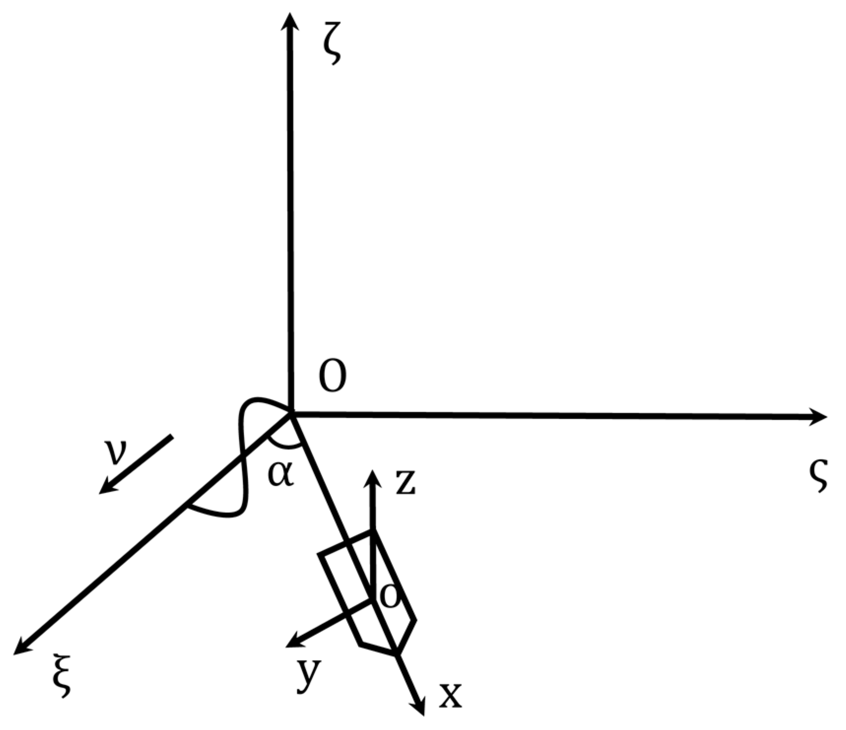
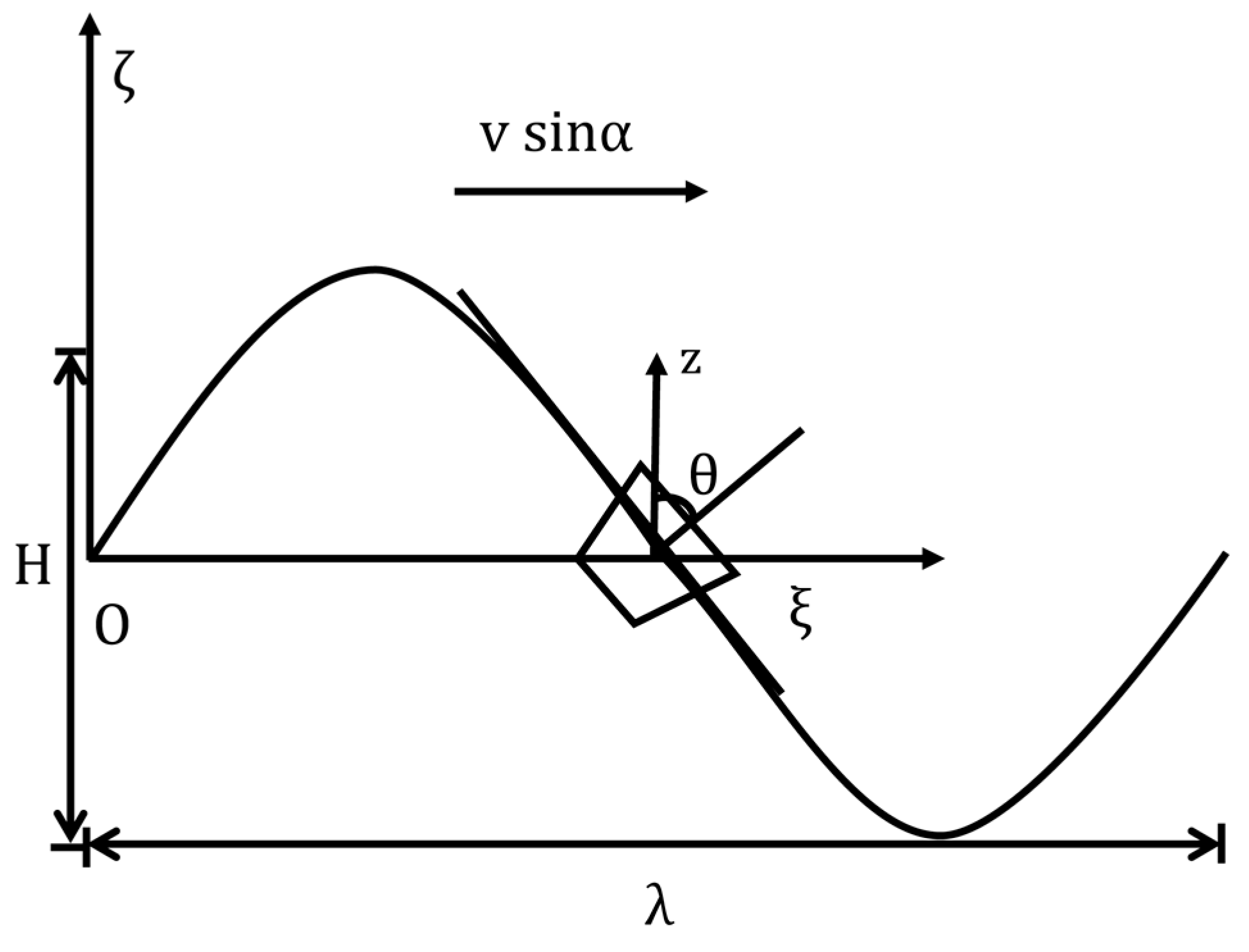
When the ship conducts atmospheric detection on the sea surface, it is usually subject to external excitation disturbances (mostly are wind, waves, and currents) and changes in space, the attitude of the lidar platform also changes. Thus, it is first necessary to establish a coordinate system to describe its spatial position and motion state. Referring to the definition of the ship’s coordinate system, assuming that the ship’s heading remains unchanged, an absolute coordinate system Oξςζ (as Figure 1 shows) that keeps the space unchanged is established. Additionally, a relative coordinate system oxyz that does not rotate but translate with the lidar platform is established at the same time (as Figure 2 shows). The Oξς plane is parallel to the still water surface, Oζ is perpendicular to the still water surface upward, and Oξ is the propagation direction of the waves on the sea surface. The relative coordinate system oxyz moves with the platform, and the origin o is fixed at the center of gravity of the lidar platform. The oxy plane is parallel to the still water surface, the ox axis points to the moving direction of the floating platform affected by external disturbances, the oy axis points to the left side of the floating platform, and the oz axis is perpendicular to the still water surface upwards. The coordinate system translates with the platform but does not rotate with the floating platform [22]. The ox axis of the lidar platform is kept in a straight line with the longitudinal axis of the ship to ensure that the rolling condition of the ship is the same as the rolling condition of the lidar platform. In order to simplify the research problem, the motion model refers to the three most common degrees of freedom of ships sailing on the sea surface. They are swaying (left and right reciprocating motion along the ship’s transverse axis oy), roll (rotational oscillation around the ship’s longitudinal axis ox), and surge (back and forth reciprocating motion along the ship’s longitudinal axis ox). Among them, roll is the most likely to occur at sea and has the largest degree of sway [23]. Therefore, this paper mainly considers the influence of ship rolling on the detection of loaded Rayleigh scattering lidar.

The actual observation angle of the lidar changes with the oscillating of the platform, which results in a change in the density of the atmosphere along the path traveled by the emitted laser beam. The signal intensity N(z) at height z that is recorded by Rayleigh scattering lidar can be expressed as follows:

$$\mathrm{N}\left(\mathrm{z}\right)=\frac{\mathrm{C}\mathsf{\rho }\left(\mathrm{z},\mathrm{R}\right)\Delta \mathrm{R}}{{\mathrm{R}}^2}$$

(1)

In the formula, C is an angle-independent quantity, including the intensity of the emitted laser, system efficiency, atmospheric scattering coefficient, etc. ρ is the density of the atmosphere. R is the line-of-sight distance, z is the altitude, and the relationship between the two is z = R cosθ. ΔR is the distance resolution.

According to the lidar signal profile N(z), the atmospheric density ρ(z, R) profile can be obtained as follows:

$$\mathsf{\rho }\left(\mathrm{z},\mathrm{R}\right)=\frac{\mathrm{N}\left(\mathrm{Rcos}\mathsf{\theta }\right){\mathrm{z}}^2}{\mathrm{N}\left({\mathrm{R}}_0\cos \mathsf{\theta }\right){\mathrm{z}}_0^2}\mathsf{\rho }\left({\mathrm{z}}_0\right)$$

(2)

$\mathsf{\rho }\left({\mathrm{z}}_0\right)$ is the atmospheric density at the reference height ${\mathrm{z}}_0$. ${\mathsf{\theta }=\mathsf{\theta }}_0+\mathsf{\phi }\left(\mathrm{t}\right)$ is the actual observation angle of the lidar, which consists of the settled observation angle ${\mathsf{\theta }}_0$ and lidar angle change φ(t) The lidar pointings with different ${\mathsf{\theta }}_0$ are as Figure 3 shows.

This paper mainly discusses the influence of the platform roll angle on temperature inversion without attitude correction. The roll model of the lidar is simplified as a sine function:

$$\mathsf{\phi }\left(\mathrm{t}\right){=\mathsf{\phi }}_0\sin \left(\mathsf{\omega }\mathrm{t}\right)$$

(3)

${\mathsf{\phi }}_0$ is the rolling amplitude value, and ω = 2π/T is the rolling frequency. T is the rolling period. These parameters refer to the rolling situation of the ship during an actual cruise.

$${\mathsf{\phi }}^{\prime }\left(\mathrm{t}\right)=\frac{{2\mathsf{\pi }\mathsf{\phi }}_0}{\mathrm{T}}\cos \left(\frac{2\mathsf{\pi }}{\mathrm{T}}\mathrm{t}\right)$$

(4)

Then, in the time Δt, the angle of the change of the optical axis of the telescope is

$${\mathsf{\phi }}^{\prime }\left(\mathrm{t}\right)\Delta \mathrm{t}=\frac{{2\mathsf{\pi }\mathsf{\phi }}_0}{\mathrm{T}}\cos \left(\frac{2\mathsf{\pi }}{\mathrm{T}}\mathrm{t}\right)\Delta \mathrm{t}$$

(5)

$$\Delta \mathrm{t}=\frac{\mathrm{s}}{\mathsf{\nu }}=\frac{2\mathrm{R}}{\mathrm{c}}$$

(6)

Δt is the time from emission to reception of a single photon in the atmosphere. Therefore, the maximum angle of the change of the optical axis of the telescope in the time Δt is:

$$\mathsf{\delta }=\frac{{2\mathsf{\pi }\mathsf{\phi }}_0\Delta \mathrm{t}}{\mathrm{T}}$$

(7)

If the field of view of the telescope is 2mrad, in order to enable the lidar in the rolling process to receive the echo signal, there are certain requirements for the rolling time period. When the detection distance R is 150 km, Δt is nearly 1 ms. Assuming that ${\mathsf{\phi }}_0$ is 30°, under this condition, the critical value of rolling period is less than 2 s. The actual rolling period is far larger than that, thus the normal reception of the number of echo photons can be guaranteed.

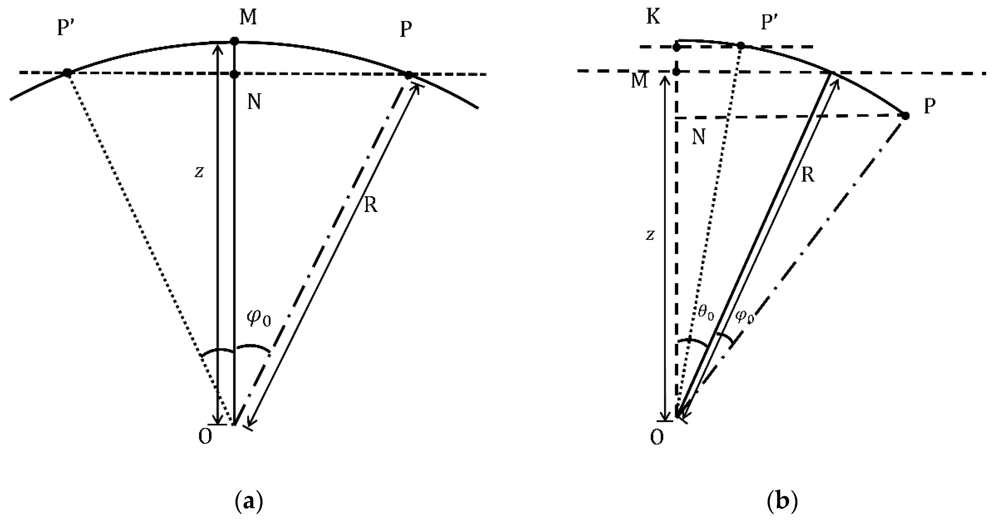
With the oscillation of the lidar, the signal position at the recorded line-of-sight height R also changes (see Figure 3 for the schematic diagram of the lidar point change), and the corresponding altitude change is $\Delta {\mathrm{z}=\mathrm{R}\cos (\mathsf{\theta }}_0{+\mathsf{\phi }}_0{)-\mathrm{R}\cos \mathsf{\theta }}_0$. The positions after swinging left and right are P’ and P. A positive or negative value of ${\mathsf{\phi }}_0$ depends on the direction of the platform oscillating. The plane is composed of the vertical direction and telescope point. ${\mathsf{\phi }}_0$ is regarded as a positive number when the telescope pointed is away from the vertical direction; in this case, the telescope direction is represented by the dash-and-dot line. In contrast, ${\mathsf{\phi }}_0$ is regarded as a negative number when the telescope is close to the vertical direction, and the dotted line is used to indicate the direction of the telescope under this condition. When the settled observation angle ${\mathsf{\theta }}_0$ is 0°, the lidar points are shown in Figure 3a. At this time, the positive and negative nature of ${\mathsf{\phi }}_0$ does not affect the density after rolling since ρ(P) = ρ(P’) is always established. When the platform does not roll, the lidar points in the vertical direction, the recorded distance is R (equal to the corresponding height z), and the atmospheric density on the transmission path is ρ(O)~ρ(M). When the platform rolls, the lidar points change to the OP or OP’ direction, the recorded distance is R (corresponding to the height ${\mathrm{R}\cos \mathsf{\phi }}_0$), and the atmospheric density on the transmission path is ρ(O)~ρ(P) or ρ(O)~ρ(P’). This means that the corresponding density in the range of height z changes from ρ(O)~ρ(M) to ρ(O)~ρ(N). ρ(M) is not equal to ρ(N) since the atmospheric density decreases as the altitude increases, and the density is the same at the same altitude, which makes the inversion temperature different.

When the settled observation angle ${\mathsf{\theta }}_0$ is not 0°, the lidar point is shown in Figure 3b. The positive and negative nature of ${\mathsf{\phi }}_0$ results in the inequality of ρ(P) and ρ(P’), which makes the density profiles different. When the platform does not roll, the lidar points an angle of ${\mathsf{\theta }}_0$ from the vertical direction, the recorded distance is R (corresponding to the height ${\mathrm{R}\cos \mathsf{\theta }}_0$), and the atmospheric density on the transmission path is ρ(O)~ρ(M). When the platform rolls, the lidar point changes to the OP or OP’ direction, the recorded distance is R (corresponding to the height ${\mathrm{R}\cos (\mathsf{\theta }}_0{+\mathsf{\phi }}_0)$), and the atmospheric density on the transmission path is ρ(O)~ρ(P) or ρ(O)~ρ(P’). That is, the corresponding density in the range of height R cosθ₀ changes from ρ(O)~ρ(M) to ρ(O)~ρ(P) or ρ(O)~ρ(P’), and neither ρ(P’) nor ρ(P) is equal to ρ(M). A bias is introduced in the temperature inversion results.

Thus, when the actual observation angle θ of the lidar changes, the recorded atmospheric density ρ on the laser transmission path also changes. This causes the corresponding density in the range of height ${\mathrm{R}\cos \mathsf{\theta }}_0$ to change from ρ(O)~ρ(M) to ρ(O)~ρ(P) or ρ(O)~ρ(P’). According to the pressure-altitude formula (Equation (8)) and the ideal gas equation of state (Equation (9)),

$$\mathrm{p}={{\displaystyle \int }}_{\mathrm{z}}^{\infty }\mathsf{\rho }\mathrm{gdz}$$

(8)

$$\mathrm{p}=\mathsf{\rho }\mathrm{RT}$$

(9)

Combining the above two formulae

$$\mathsf{\rho }\left(\mathrm{z}\right){\mathrm{R}}_{\mathrm{d}}\mathrm{T}\left(\mathrm{z}\right)={{\displaystyle \int }}_{\mathrm{z}}^{\infty }\mathsf{\rho }\left(\mathrm{z}\right)\mathrm{gdz}={{\displaystyle \int }}_{\mathrm{z}0}^{\infty }\mathsf{\rho }\left(\mathrm{z}\right)\mathrm{gdz}+{{\displaystyle \int }}_{\mathrm{z}}^{\mathrm{z}0}\mathsf{\rho }\left(\mathrm{z}\right)\mathrm{gdz}$$

(10)

$$\mathsf{\rho }\left(\mathrm{z}\right){\mathrm{R}}_{\mathrm{d}}\mathrm{T}\left(\mathrm{z}\right){=\mathsf{\rho }}_{\mathrm{z}0}{\mathrm{R}}_{\mathrm{d}}{\mathrm{T}}_{\mathrm{z}0}+{{\displaystyle \int }}_{\mathrm{z}}^{\mathrm{z}0}\mathsf{\rho }\left(\mathrm{z}\right)\mathrm{gdz}$$

(11)

Therefore, the temperature calculation formula at height z is

$$\mathrm{T}\left(\mathrm{z}\right)=\frac{\left({\mathsf{\rho }}_{\mathrm{z}0}{\mathrm{T}}_{\mathrm{z}0}+\frac{1}{{\mathrm{R}}_{\mathrm{d}}}{{\displaystyle \int }}_{\mathrm{z}}^{\mathrm{z}0}\mathsf{\rho }\left(\mathrm{z}\right)\mathrm{gdz}\right)}{\mathsf{\rho }\left(\mathrm{z}\right)}$$

(12)

g is the acceleration due to gravity;

${\mathsf{\rho }}_{\mathrm{z}0}$ is the atmospheric density at the reference altitude;

${\mathrm{T}}_{\mathrm{z}0}$ is the atmospheric temperature at the reference altitude;

${\mathrm{R}}_{\mathrm{d}}$ is the gas constant of dry air.

To evaluate the influence of the change in laser point angle on the temperature measurement accuracy, the lidar signal is simulated according to the atmospheric density output of the NRLMSISE-00 model. Then, the lidar signal is substituted into the temperature inversion algorithm, and the temperature at the top of the detection height is utilized as the reference temperature to invert the temperature profile. Finally, the inversion temperature profile is compared with the temperature profile output of the NRLMSISE-00 model. This avoided the inversion temperature deviation caused by the deviation in the temperature value at the top of the detection height. The specific method is described as follows: substitute the lidar’s angle change formula ${\mathsf{\theta }=\mathsf{\theta }}_0+\mathsf{\phi }\left(\mathrm{t}\right)$ into the atmospheric density $\mathsf{\rho }\left(\mathrm{R}\cos \mathsf{\theta }\right)$ to obtain the atmospheric density profile after angle conversion. According to the simulated atmospheric density profile, the atmospheric echo photons are obtained, and then, the atmospheric temperature profile can be obtained by inputting the atmospheric photon profile into the inversion algorithm. Comparing it with the NRLMSISE-00 model, the temperature deviation caused by the oscillating of the ship platform is obtained.

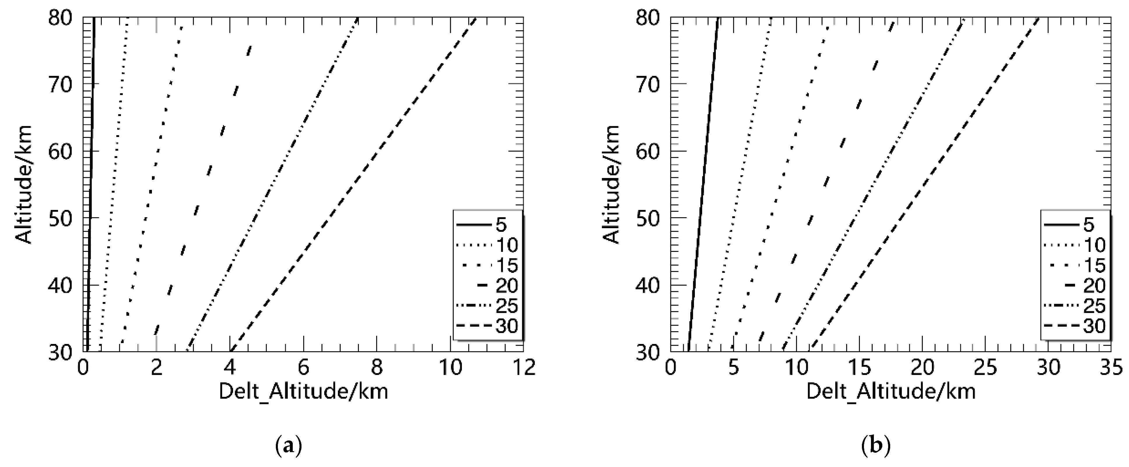
When the platform rolls, the line-of-sight distance R for the telescope to receive echo photons is not affected, and the corresponding height ${\mathrm{R}\cos \mathsf{\theta }}_0$ changes with the roll angle. When the actual observation angle θ of the lidar changes, the calculation result of its height change is shown in Figure 4. ${\mathrm{R}\cos \mathsf{\theta }}_0$ is the altitude shown on the Y-axis in the figure, and ${\mathrm{R}\cos (\mathsf{\theta }}_0{+\mathsf{\phi }}_0{)-\mathrm{R}\cos \mathsf{\theta }}_0$ is the height change and is represented on the X-axis in subfigures a and b in Figure 4 show the variation in height with the change in the amplitudes of the roll angles at different settled observation angles (0° and 30°). The roll amplitude is increased from 5° to 30° in 5° intervals. The figure shows that the amount of height change increases with height and angle. The variation in altitude between 0 and 80 km is less than 0.5 km at a ${\mathsf{\theta }}_0$ value of 0 and ${\mathsf{\phi }}_0$ value of 5. When ${\mathsf{\theta }}_0$ is 0° and ${\mathsf{\phi }}_0$ is 10°, the height difference within 0–80 km is less than 2 km. When ${\mathsf{\theta }}_0$ is 30° and ${\mathsf{\phi }}_0$ is 5°, the deviation in altitude within 0–80 km is less than 4 km.

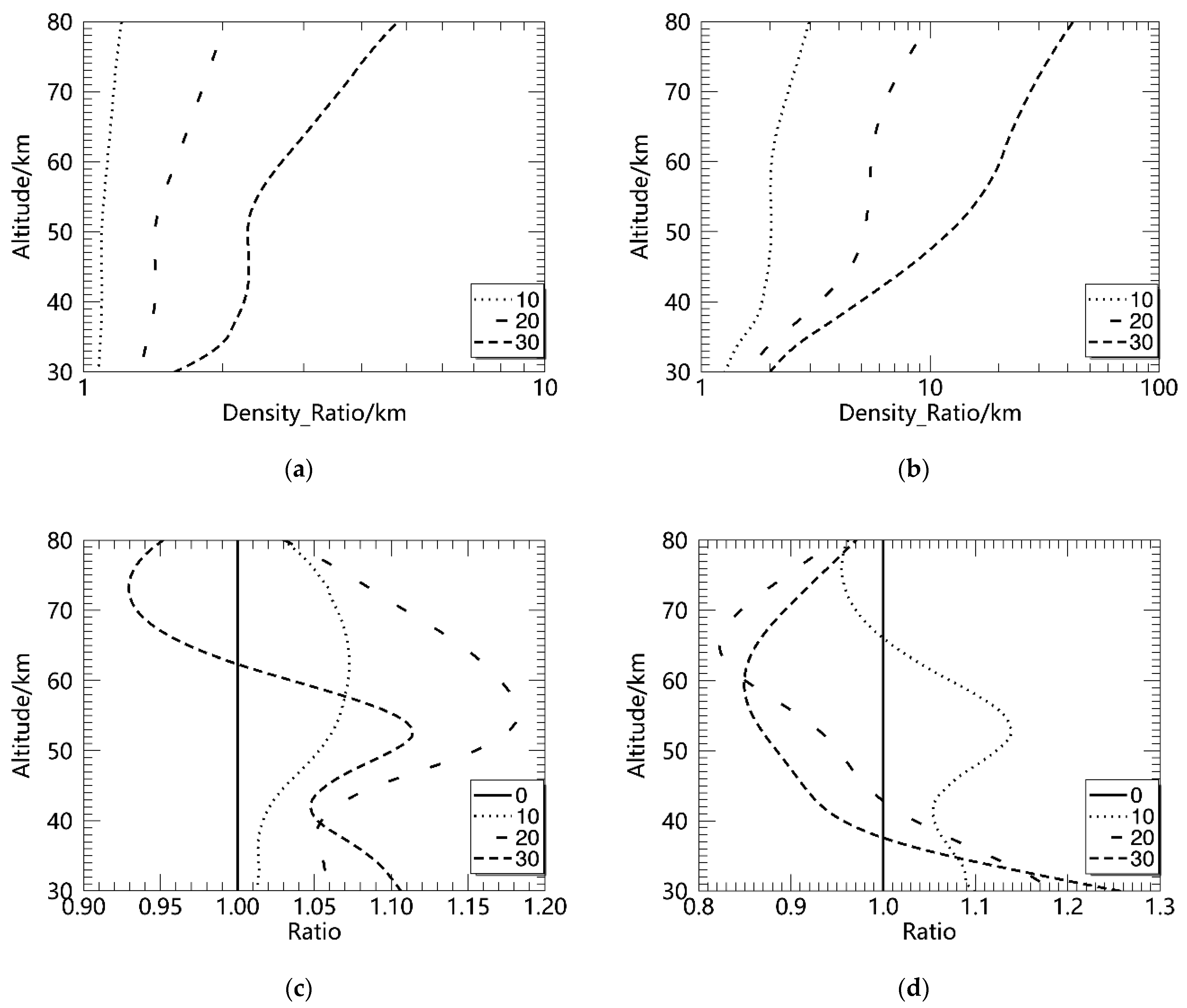
The variation trend of density and temperature relative to model temperature under a certain roll angle is shown in Figure 5a,b in Figure 3 show the density ratio when the amplitudes of the roll angles are 10°, 20°, and 30° at different settled observation angles (0° and 30°). The density ratio is defined as the ratio of the density profile after rolling with an amplitude of ${\mathsf{\phi }}_0$ to the density profile without rolling. ${\mathrm{R}\cos \mathsf{\theta }}_0$ is the altitude shown on the Y-axis in the figure, and the X-axis is utilized to demonstrate the ratio of the density. The graph shows that the ratio of densities increases with height and angle. When the amplitudes of roll angles are 10°, 20°, and 30°, the density changes in the range of 30–80 km are all within the same order of magnitude at θ = 0°. When ${\mathsf{\theta }}_0$ is 30°, the ratio of density at 80 km at ${\mathsf{\phi }}_0=0°$ is an order of magnitude higher than that at 30°. Figure 5c,d show the ratio (inversion temperature divided by model temperature) of temperature when the amplitudes of the roll angles are 10°, 20°, and 30° at different settled observation angles (0° and 30°). ${\mathrm{R}\cos \mathsf{\theta }}_0$ is the altitude shown on the Y-axis, and the ratio of the temperature is shown on the X-axis in the figure. The graphs show that when the roll angle increases, the inversion temperature relative to the model temperature gradually changes from a positive bias to a positive bias and negative bias. The height interval of the negative bias expands with increasing angle, that is, the variation range of the inversion temperature increases. This shows that the rolling of the platform may have a greater impact on the temperature inversion results, and the errors caused by the periodic oscillating of the platform are simulated below.

3. Results and Discussion

3.1. Accuracy Check of Inversion Results

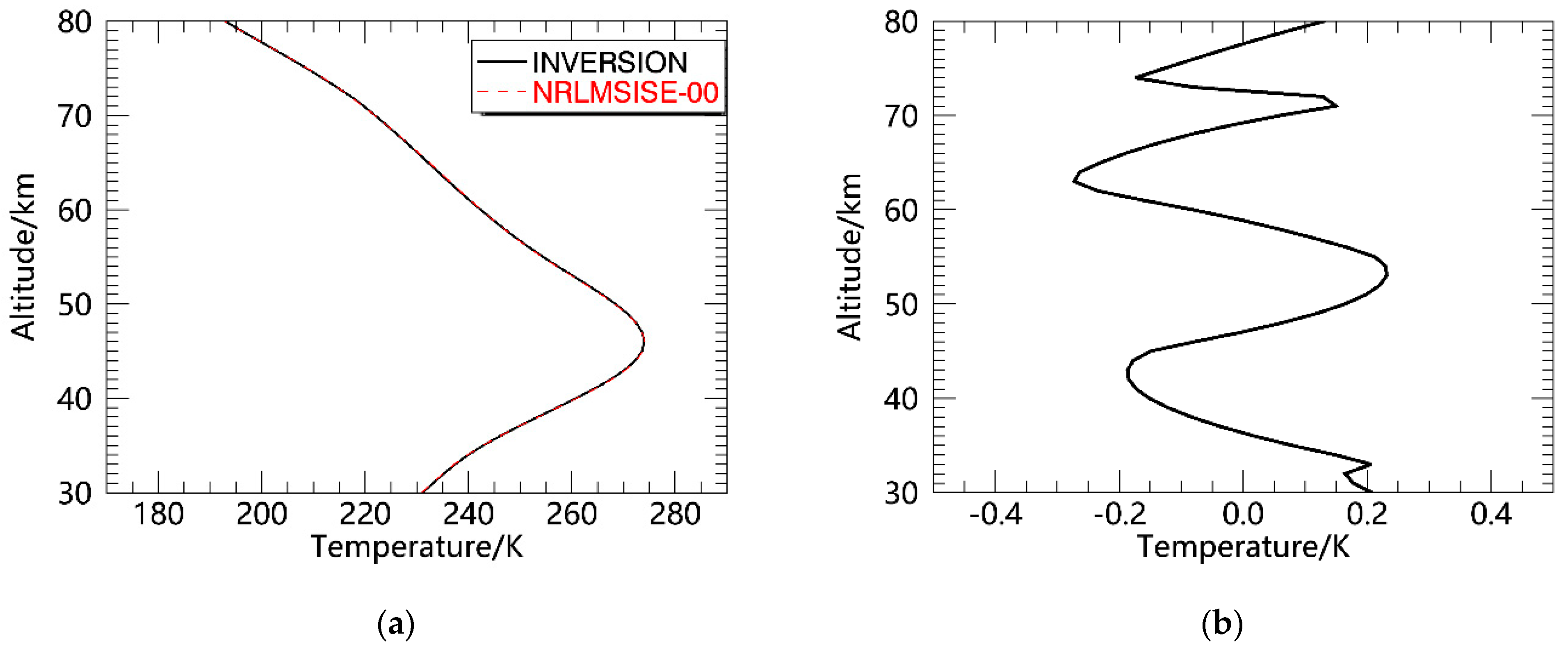
First, profiles of atmospheric density and temperature versus altitude are obtained from the model (the distance resolution is 1 km). Then, the atmospheric echo photon number profile is simulated by substituting the density profile into the photon simulation program under different settled observation angles and rolling angles. Finally, the atmospheric temperature is calculated by a temperature inversion algorithm with one-hour-integrated photons. The deviation in temperature between the inversion results and the model is wanted. When the actual observation angle of the lidar is 0° (the settled observation angle is 0° and the platform does not roll). The simulated results are shown in Figure 6 below. Figure 6a shows the comparison of the inversion atmospheric temperature and the temperature of the NRLMSISE-00 with altitude, which ranges from 30 to 80 km when the ship platform does not roll. The inversion results and the model results basically coincide with the change in height, and they have good consistency. In the 30–45 km altitude range, the stratospheric temperature increases gradually with altitude due to the absorption of UV radiation by ozone. In the range of 45–80 km, the temperature of the mesosphere gradually decreases with height. The deviation in the model temperature from the inversion temperature is shown in Figure 6b. The temperature inversion is calculated with a temperature of 90 km as a reference. The maximum deviation in the height range of 30–80 km is 0.27 K, and the average deviation is 0.004 K. The reason for the difference is that in the NRLMSISE-00 model, the atmospheric density values of the main components (N₂, O₂, O, N, etc.) are calculated based on the calculated temperature. The method in this paper uses atmospheric density to invert atmospheric temperature, and the average relative molecular weight needs to be derived from the accumulation of model atmospheric components. However, the model lacks detection data for atmospheric compositions above 62.5 km. During modeling, the number density of each component is corrected to achieve a smooth transition from the middle layer to the low thermal layer [24]. This results in a decrease in the average molecular molar mass at altitudes above 62.5 km. The deviation between the inversion temperature and the model temperature is introduced when integrating down from 90 km according to equation (12). When the input geographic location of the model is set to 40.3°N, 116.7°E, and the time is 23:30:00 on May 1, 2021, the average mass of the largest molecule decreases by 1.28‰. The temperature of the model in the height range of 30–90 km has a minimum of 170.99 K and a maximum of 274.11 K. The temperature deviations under the same ratio are approximately 0.22 K and 0.35 K, so the maximum temperature deviation in the inversion results of 0.27 K is within a reasonable range.

3.2. Deviation between the Inversion Temperature and the Model When the Actual Observed Angle Changes Periodically with Time

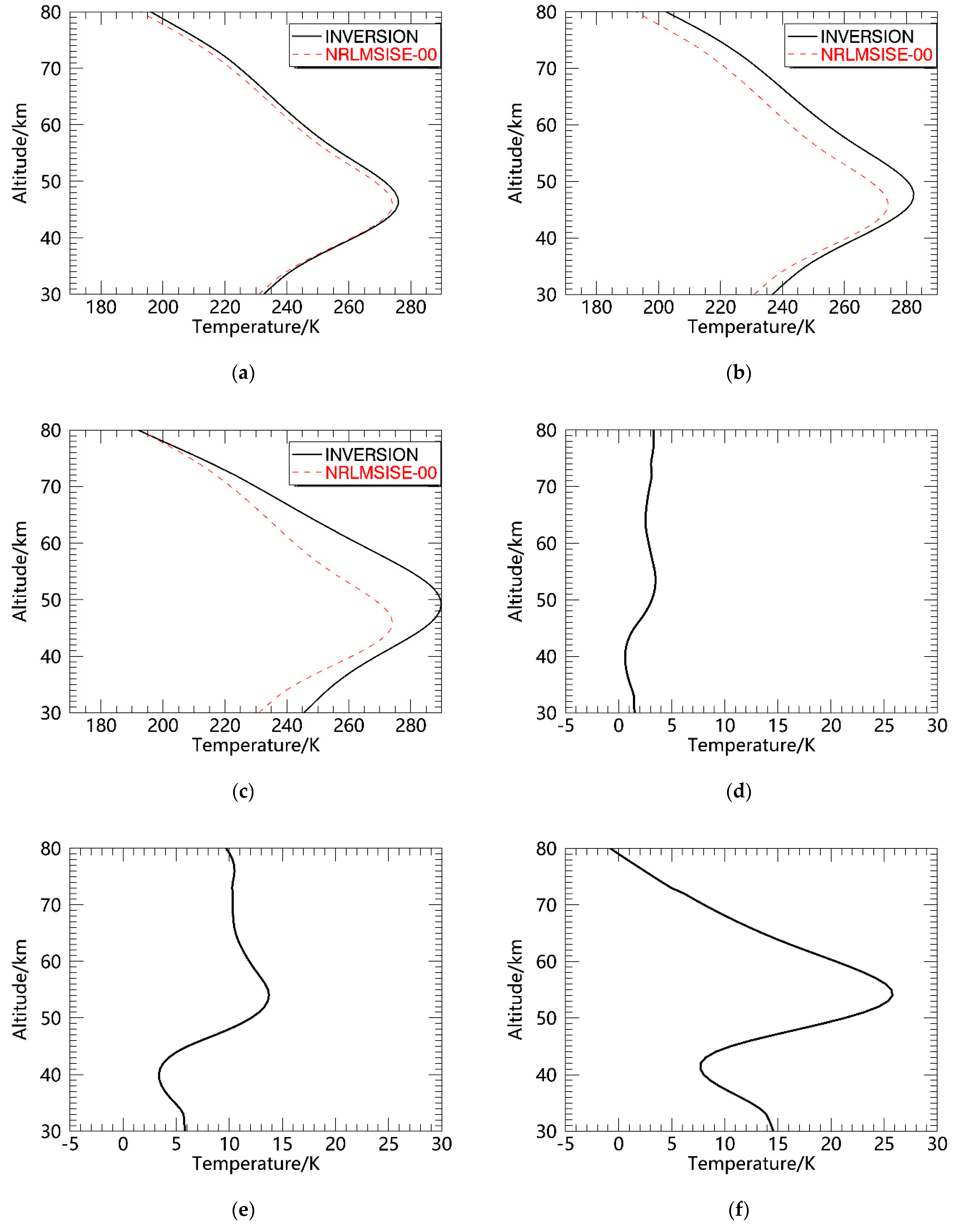
When the settled observation angle is 0°, the simulated ship platform rolls periodically, and the platform swings left and right in the plane of the wave propagation direction. φ(t) is a sine function that changes with time to represent the angle change, and the amplitude of the rolling angle is 10°, 20°, and 30°. The temperature profiles at the corresponding angles obtained by inversion are shown in Figure 7. Figure 7a–c are the inversions of atmospheric temperature and NRLMSISE-00 model temperature with altitude when the roll angle amplitudes are 10°, 20°, and 30° within a range of 30–80 km, respectively. At different roll angles, the inversion value of atmospheric temperature agrees with the variation trend in the model value with height. The inversion value of atmospheric temperature is basically larger than the model temperature, and with the increase in ${\mathsf{\phi }}_0$, the deviation between the two is larger. Figure 7d–f show the difference between the inversion atmospheric temperature and the model temperature when the amplitudes of roll angles are 10°, 20°, and 30° within 30–80 km, respectively. When the amplitude of the roll angle is 10°, the inversion temperature is positively biased relative to the model temperature, the average deviation is 2.35 K, and the maximum temperature deviation is 3.47 K, which appears at 53 km. When the amplitude of the roll angle is 20°, the inversion temperature is positively biased relative to the model temperature, the average deviation is 9.09 K, and the maximum temperature deviation is 13.73 K, which appears at 54 km. When the amplitude of the roll angle is 30°, the inversion temperature relative to the model temperature is positively biased above 79 km and negatively biased below 79 km. The average deviation is 12.95 K, and the maximum temperature deviation is 22.78 K, which appears at 54 km. With increasing height, the overall trend first declines, then rises and then declines. The larger the angle is, the larger the deviation in the temperature. The maximum occurs near the stratopause.

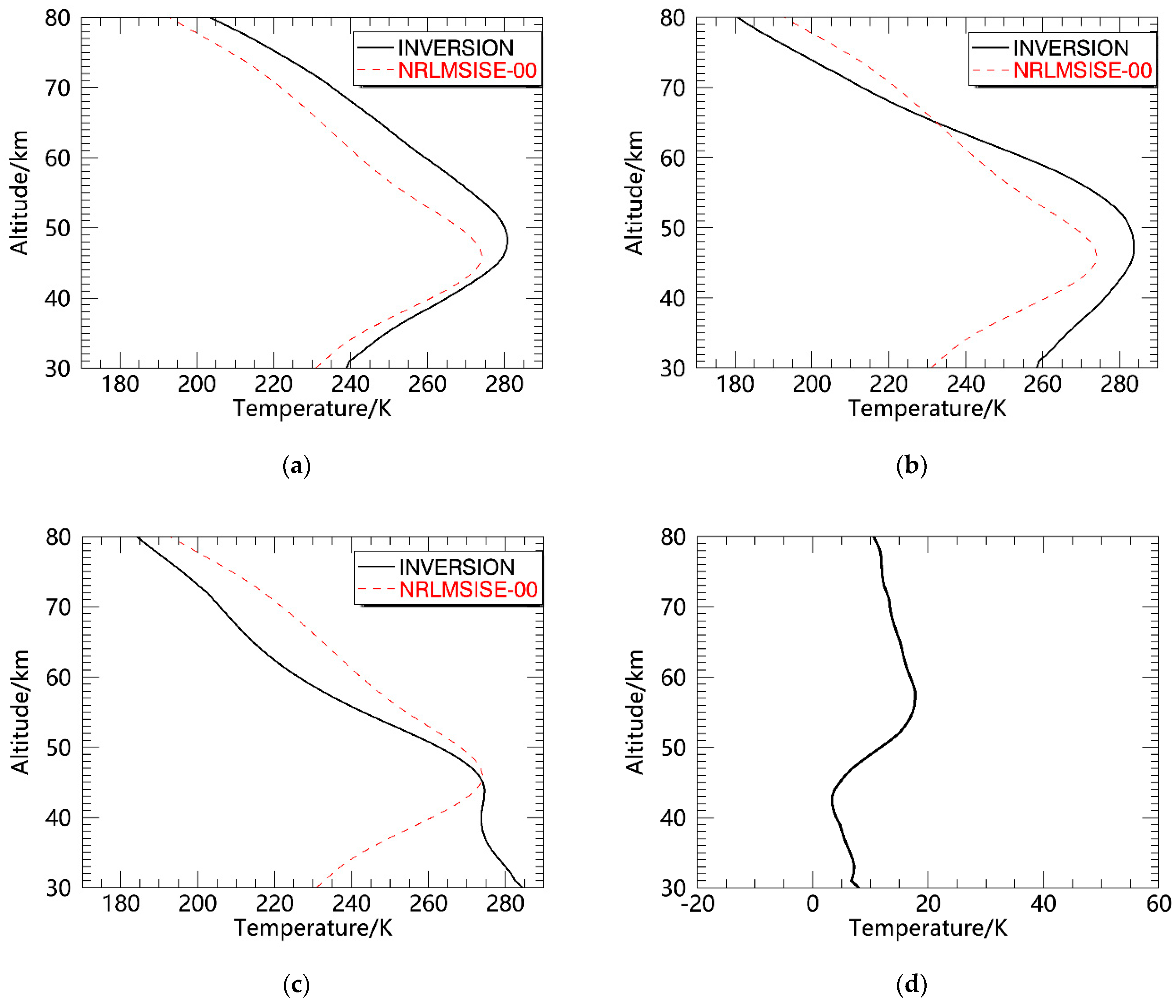
When the settled observation angle is 30°, the amplitude of the rolling angle is 10°, 20°, and 30°. The comparison of the atmospheric temperature between the inversion and NRLMSISE-00 model within 30–80 km is shown in Figure 8a–c, and their difference is shown in Figure 8d–f. The graph shows that there is a large deviation between the inversion value and the model value under a certain observation angle, and the deviation distribution of the inversion value and the model value changes with the change in height under different roll angles. When the amplitude of the roll angle is 10°, the inversion temperature is positively biased relative to the model temperature, the average deviation is 11.05 K, and the maximum temperature deviation is 11.75 K, which appears at 57 km. When the amplitude of the roll angle is 20°, the inversion temperature above 66 km is negatively biased relative to the model temperature, and the inversion temperature below 66 km is positively biased. The average deviation is 13.88 K, and the maximum temperature deviation is 27.49 K, which appears at 30 km. When the amplitude of the roll angle is 30°, the inversion temperature above 46 km is negatively biased relative to the model temperature, and the inversion temperature below 46 km is positively biased. The average deviation is 16.12 K, and the maximum temperature deviation is 53.50 K, which appears at 30 km. When the platform rolls, the maximum temperature deviation and the average deviation between the inversion temperature and the model temperature both increase with increasing roll angle.

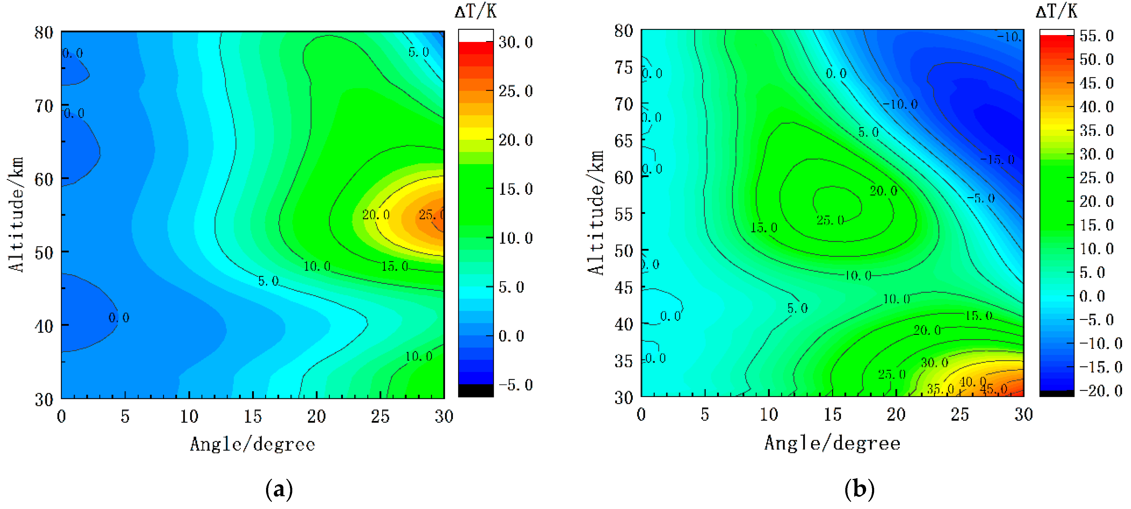
Figure 9a shows the temperature deviation as the roll angle amplitude varies from 0° to 30° (in 1° intervals) when the observation angle is set at 0°. When the amplitude of the roll angle is less than 10°, the temperature deviation is less than 5 K. The temperature deviation increases as the amplitude of the roll angle increases, and maximum temperature deviation occurs near the stratopause. When the amplitude of the roll angle is 30°, there is a negative bias at 80 km. Figure 9b shows the temperature deviation as the roll angle amplitude varies from 0° to 30° (in 1° intervals) when the observation angle is set at 30°. The temperature deviation increases with increasing rolling angle. When the amplitude of the roll angle is greater than 13°, the temperature difference at 80 km has a negative deviation, and the height range of the negative deviation extends downward from 80 km with the increase in the roll angle. When the amplitude of the roll angle is less than 19°, the maximum temperature deviation occurs in the stratosphere, and when the amplitude of the roll angle is greater than or equal to 19°, the maximum temperature deviation appears at 30 km. Thus, when the settled observation angle remains constant, the larger the rolling angle is, the larger the maximum temperature deviation is.

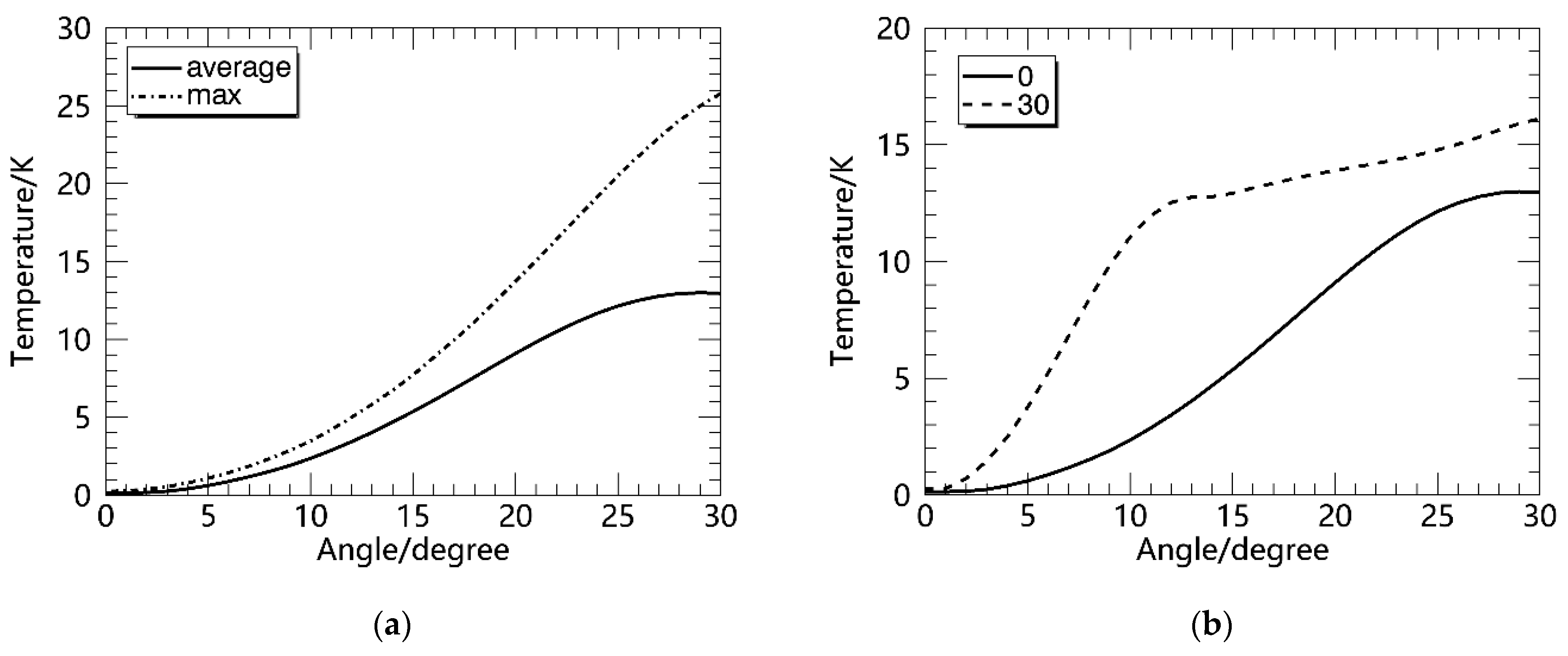
Figure 10a shows the average and maximum deviation in temperature as the roll angle amplitude varies from 0° to 30° (in 1° intervals) when the observation angle is set at 0°. The dash-and-dot line represents its maximum deviation, and the solid line represents its average deviation. They both increase with increasing angle. When the maximum temperature difference is less than 1 K, the amplitude of the roll angle is 4°. When the average temperature difference is less than 1 K, the amplitude of the roll angle is 6°. The solid and dashed lines in Figure 10b are the average deviations between the inversion temperature and the model temperature when the settled observation angle is 0° and 30°, respectively. This shows that under the same settled observation angle, the larger the roll angle is, the larger the average deviation. Under the same rolling angle, the larger the settled observation angle is, the larger the average deviation.

4. Conclusions

In this paper, the influence of observation angle changes caused by ship rolling on the inversion temperature is analyzed and studied based on ship-borne Rayleigh scattering lidar for atmospheric temperature detection within 30–80 km at sea, and the following conclusions were obtained as the result of this study:

(1) When the observation angle is set to be constant, the larger the roll angle is, the larger the average deviation and maximum deviation in the inversion temperature are. When the settled observation angle is 0°, the maximum temperature difference is less than 1 K, while the amplitude of the roll angle is 4°. The average temperature difference is limited to 1 K, corresponding to a roll angle amplitude of 6°. The maximum deviation appears at the stratopause. When the settled observation angle is 30°. When the average temperature difference is less than 1 K, the corresponding roll angle amplitude is 2°, and all the maximum temperature deviations are greater than 1 K. The maximum temperature deviation takes ${\mathsf{\phi }}_0=19°$ as the turning point. When ${\mathsf{\phi }}_0$ is less than 19°, the maximum temperature deviation occurs in the stratopause, and when ${\mathsf{\phi }}_0$ is greater than or equal to 19°, the maximum temperature deviation occurs at 30 km.

(2) When the roll angle is constant, the larger the settled observation angle is, the larger the average deviation and maximum deviation in the inversion temperature will be. When the roll angle amplitude is 10°, the average deviation corresponding to setting the observation angle to 0° is 2.35 K, and the maximum deviation is 3.47 K. The average deviation corresponding to setting the observation angle to 30° is 11.04 K, and the maximum deviation is 17.74 K. When the roll angle amplitude is 20°, the average deviation corresponding to setting the observation angle to 0° is 9.09 K, and the maximum deviation is 13.73 K. The average deviation corresponding to setting the observation angle to 30° is 13.88 K, and the maximum deviation is 27.50 K. When the roll angle amplitude is 30°, the average deviation corresponding to setting the observation angle to 0° is 12.95 K, and the maximum deviation is 25.78 The average deviation corresponding to setting the observation angle to 30° is 16.12 K, and the maximum deviation is 53.50 K.

Therefore, when the rolling amplitude of the ship is large, it is necessary to correct the data or stabilize the attitude of the lidar platform before the temperature inversion to obtain temperature data that are more in line with the actual situation.

References

1. Weitkamp, C. Lidar: Range-Resolved Optical Remote Sensing of the Atmosphere; Springer: Berlin/Heidelberg, Germany, 2005; pp. 273–306. [Google Scholar]
2. Yan, Z.; Hu, X.; Guo, W.; Guo, S.; Cheng, Y.; Zhang, B.; Chen, Z.; Zhao, W. Near space Doppler lidar techniques and applications (Invited). Infrared Laser Eng. 2021, 50, 20210100. [Google Scholar]
3. Wing, R.; Martic, M.; Triplett, C.; Hauchecorne, A.; Porteneuve, J.; Keckhut, P.; Courcoux, Y.; Yung, L.; Retailleau, P.; Cocuron, D. Gravity Wave Breaking Associated with Mesospheric Inversion Layers as Measured by the Ship-Borne BEM Monge Lidar and ICON-MIGHTI. Atmosphere 2021, 12, 1386. [Google Scholar] [CrossRef]
4. Suzuki, S.; Lübken, F.-J.; Baumgarten, G.; Kaifler, N.; Eixmann, R.; Williams, B.P.; Nakamura, T. Vertical propagation of a mesoscale gravity wave from the lower to the upper atmosphere. J. Atmos. Sol.-Terr. Phys. 2013, 97, 29–36. [Google Scholar] [CrossRef]
5. Sox, L.; Wickwar, V.B.; Yuan, T.; Criddle, N.R. Simultaneous Rayleigh-scatter and sodium resonance lidar temperature comparisons in the mesosphere-lower thermosphere. Atmospheres 2018, 123, 10688–10706. [Google Scholar] [CrossRef]
6. Taori, A.; Kamalakar, V.; Raghunath, K.; Rao, S.V.B.; Russell, J.M., III. Simultaneous Rayleigh lidar and airglow measurements of middle atmospheric waves over low latitudes in India. J. Atmos. Sol.-Terr. Phys. 2012, 78–79, 62–69. [Google Scholar] [CrossRef]
7. Guharay, A.; Sekar, R. Seasonal characteristics of gravity waves in the middle atmosphere over Gadanki using Rayleigh lidar observations. J. Atmos. Sol.-Terr. Phys. 2011, 73, 1762–1770. [Google Scholar] [CrossRef]
8. Di Liberto, L.; Cairo, F.; Fierli, F.; Di Donfrancesco, G.; Viterbini, M.; Deshler, T.; Snels, M. Observation of polar stratospheric clouds over McMurdo (77.85° S, 166.67° E) (2006–2010). J. Geophys. Res.-Atmos. 2014, 119, 5528–5541. [Google Scholar] [CrossRef] [Green Version]
9. Fong, W.; Chu, X.; Lu, X.; Fuller-Rowell, T.J.; Codrescu, M.; Richmond, A.D.; Yu, Z.; Roberts, B.; Chen, C. Winter temperature and tidal structures from 2011 to 2014 at mcmurdo station: Observations from fe boltzmann temperature and rayleigh lidar. EPJ Web Conf. 2016, 119, 12003. [Google Scholar] [CrossRef]
10. Ardalan, M.; Keckhut, P.; Hauchecorne, A.; Wing, R.; Meftah, M.; Farhani, G. Updated Climatology of Mesospheric Temperature Inversions Detected by Rayleigh Lidar above Observatoire de Haute Provence, France, Using a K-Mean Clustering Technique. Atmosphere 2022, 13, 814. [Google Scholar] [CrossRef]
11. Yue, C.; Yang, G.; Wang, J.; Guan, S.; Du, L.; Cheng, X.; Yang, Y. Lidar observations of the middle atmospheric thermal structure over north China and comparisons with TIMED/SABER. J. Atmos. Sol.-Terr. Phys. 2014, 120, 80–87. [Google Scholar] [CrossRef]
12. Chang, Q.; Yang, G.; Song, J.; Gong, S. Studying the Stability of the Middle Atmosphere (30~60 km) over Wuhan by Rayleigh Lidar. Chin. Sci. Bull. 2005, 50, 2786–2789. [Google Scholar]
13. Qiao, S.; Pan, W.; Ban, C.; Zhang, H. Mesospheric density measured by Rayleigh lidar over Golmud. Infrared Laser Eng. 2018, 47, 31–36. [Google Scholar]
14. Dou, X.; Han, Y.; Sun, D.; Xia, H.; Shu, Z.; Zhao, R.; Shangguan, M.; Guo, J. Mobile Rayleigh Doppler lidar for wind and temperature measurements in the stratosphere and lower mesosphere. Opt. Express. 2014, 22, A1203–A1221. [Google Scholar] [CrossRef]
15. Yan, Z.; Hu, X.; Guo, W.; Guo, S.; Cheng, Y.; Gong, J.; Yue, J. Development of a mobile Doppler lidar system for wind and temperature measurements at 30–70 km. J. Quant. Spectrosc. Radiat. Transf. 2017, 188, 52–59. [Google Scholar] [CrossRef]
16. Zhao, W.; Hu, X.; Yan, Z.; Pan, W.; Guo, W.; Yang, J.; Du, X. Atmospheric Gravity Wave Potential Energy Observed by Rayleigh Lidar above Jiuquan (40°N, 95°E), China. Atmosphere 2022, 13, 1098. [Google Scholar] [CrossRef]
17. Zhao, W.; Hu, X.; Pan, W.; Yan, Z.; Guo, W. Mesospheric Gravity Wave Potential Energy Density Observed by Rayleigh Lidar above Golmud (36.25°N, 94.54°E), Tibetan Plateau. Atmosphere 2022, 13, 1084. [Google Scholar] [CrossRef]
18. Hauchecorne, A.; Chanin, M.L.; Keckhut, P. Climatology and trends of the middle atmospheric-temperature(33~87km) as seen by Rayleigh lidar over the south of France. J. Geophys. Res. 1991, 96, 15297–15309. [Google Scholar] [CrossRef]
19. Zhang, Y.; Wu, T.; Zhang, X.; Sun, Y.; Wang, Y.; Li, S.; Li, X.; Zhong, K.; Yan, Z.; Xu, D.; et al. Rayleigh Lidar Signal Denoising Method Combined with WT, EEMD and LOWESS to Improve Retrieval Accuracy. Remote Sens. 2022, 14, 3270. [Google Scholar] [CrossRef]
20. She, C.-Y.; Friendman, J.S. Atmospheric Lidar Fundamentals: Laser Light Scattering from Atoms and Linear Molecules; Cambridge University Press: New York, NY, USA, 2022; pp. 150–155. [Google Scholar]
21. Wing, R.; Martic, M.; Hauchecorne, A.; Porteneuve, J.; Keckhut, P.; Courcoux, Y.; Yung, L.; Retailleau, P.; Cocuron, D. Atmospheric density and temperature vertical profile retrieval for flight-tests with a Rayleigh lidar on-board the French advanced test range ship Monge. Atmosphere 2020, 11, 75. [Google Scholar] [CrossRef] [Green Version]
22. Li, H.; Lu, J. Ship Parametric Excitation Rolling Motion in a Regular Longitudinal Wave. Ship Boat 2011, 22, 16–20. [Google Scholar]
23. Xiaojun, L.; Ran, Z.; Lequn, Z.; Xueyi, L.; Bin, Y. Analysis of rolling motion of semi-submerged ship in wind and waves. China Water Transport 2018, 8, 62–64. [Google Scholar] [CrossRef]
24. Picone, J.M.; Hedin, A.E.; Drob, D.P.; Aikin, A.C. NRLMSISE-00 empirical model of the atmosphere: Statistical comparison and scientific issues. J. Geophys. Res. 2002, 107, 1468. [Google Scholar] [CrossRef]
Figure 1. The coordinate diagram of floating platform.
Remotesensing 14 05033 g001
Figure 2. The coordinate diagram of floating platform.
Remotesensing 14 05033 g002
Figure 3. (a) The pointing diagram of lidar at θ 0 = 0 ° ; (b) the pointing diagram of lidar at θ 0 = 30 ° .
Remotesensing 14 05033 g003
Figure 4. (a) The deviation in altitude when the settled observation angle is 0° and the roll amplitude is increased from 5° to 30° in 5° intervals within 30–80 km. (b) The deviation in altitude when the settled observation angle is 30° and the roll amplitude is increased from 5° to 30° in 5° intervals within 30–80 km.
Remotesensing 14 05033 g004
Figure 5. (a) The density ratio when the amplitudes of the roll angles are 10°, 20°, and 30° at θ 0 = 0 ° from 30 km to 80 km. (b) The density ratio when the amplitudes of the roll angles are 10°, 20°, and 30° at θ 0 = 30 ° from 30 km to 80 km. (c) The temperature ratio when the amplitudes of the roll angles are 10°, 20°, and 30° at θ 0 = 0 ° from 30 km to 80 km. (d) The temperature ratio when the amplitudes of the roll angles are 10°, 20°, and 30° at θ 0 = 30 ° from 30 km to 80 km.
Remotesensing 14 05033 g005
Figure 6. (a) Comparison of temperature between the inversion and NRLMSISE-00 model from 30 km to 80 km without rolling; (b) deviation in temperature between the inversion and NRLMSISE-00 model from 30 km to 80 km without rolling.
Remotesensing 14 05033 g006
Figure 7. (ac) Comparison of temperature profiles between the inversion and NRLMSISE-00 model from 30 km to 80 km with roll angles of 10°, 20°, and 30° on the precondition that the settled observation angle is 0°. (df) Deviation in temperature profiles between the inversion and NRLMSISE-00 model from 30 km to 80 km with roll angles of 10°, 20°, and 30° on the precondition that the settled observation angle is 0°.
Remotesensing 14 05033 g007
Figure 8. (ac) Comparison of temperature between the inversion and NRLMSISE-00 model from 30 km to 80 km with roll angles of 10°, 20°, and 30° on the precondition that the settled observation angle is 30°; (df) Deviation in temperature between the inversion and NRLMSISE-00 model from 30 km to 80 km with roll angles of 10°, 20°, and 30° on the precondition that the settled observation angle is 30°.
Remotesensing 14 05033 g008aRemotesensing 14 05033 g008b
Figure 9. (a) The deviations in temperature vary from 0° to 30° at θ 0 = 0 ° ; (b) the deviations in temperature vary from 0° to 30° at θ 0 = 30 ° .
Remotesensing 14 05033 g009
Figure 10. (a) The average (solid line) and max (dash-and-dot line) deviations in temperature vary from 0° to 30° at θ 0 = 0 ° ; (b) the average deviations in temperature vary from 0° to 30° at θ 0 = 0 ° (solid line) and θ 0 = 30 ° (dashed line).
Remotesensing 14 05033 g010
Publisher’s Note: MDPI stays neutral with regard to jurisdictional claims in published maps and institutional affiliations.