Abstract
Mining-induced ground movement is a complicated nonlinear process and a regional geological hazard. Time series in Earth sciences are often characterized as self-affine, long-range persistent, where the power spectra exhibit a power-law dependence on frequency. Whether there exists a periodic signal and a fundamental frequency in the time series is significant in analyzing ground-movement patterns. To evaluate whether a power law describes the power spectra of a ground-movement time series and whether a fundamental frequency exists, GPS monitoring records taken over 14.5 years describing ground movement in the Jinchuan Nickel Mine, China, were analyzed. The data sets consisted of 500 randomly selected GPS monitoring points, spanning the April 2001–October 2015 time period. Whether a periodic signal in the ground movements existed was determined through the autocorrelation function. The power spectra of the ground-movement time series were found to display power-law behavior over vastly different timescales. The spectral exponents of the horizontal and vertical displacements ranged from 0.47 to 3.58 and from 0.43 to 3.37, with mean values of 2.05 and 1.79, respectively. The ground movements of minefields No.1 and No.2 had 1.1-month and 1.4-month fundamental periods, respectively. Together with a discussion of the underlying mechanisms of power-law behavior and relevant influencing factors, these results indicate that ground-movement time series are a type of self-affine time series that exhibit long-range persistence and scale invariance and show a complex periodicity. These conclusions provide a basis for predicting land subsidence in the study area over a timescale.
1. Introduction
Ground movement, which changes the Earth’s surface, can be induced by earthquakes, volcanoes and landslides. It can also be caused by underground mining, groundwater extraction, underground construction and other human activities [,,,]. Mining-induced ground movement is usually nonlinear, complex and dynamic due to complex interactions in the host rock, the inhomogeneous distribution of topsoil, the mining rate and mining method, ever-changing mining areas and stress fields. Considerable progress has been made in studying the characteristics, physical processes, prediction methods and factors associated with mining-induced ground movements [,,,]. To forecast mining-induced ground movements, traditional prediction methods use analytical or numerical simulations to approximate a static expression of movement. These methods oversimplify the problem and only deal with ideal conditions. Typically, the nonlinear interaction between each rock mass unit within the system is ignored, and the dynamic evolution of ground movement cannot be modeled. To investigate only the transient stability state and ignore the dynamic and non-equilibrium processes affecting underground mining is untenable. Some researchers have described mine subsidence as a self-organized process [,]. Although the fractal increments of dynamic subsidence induced by underground mining have been studied, the physical mechanisms underlying them are still unclear.
When dealing with movement processes, time introduces an additional co-ordinate axis to space, and the ground-movement time series contains significant information about the rock mass system. Further complexity is added when such a process is observed on small spatiotemporal scales, but estimates are also needed for very large ones. If a fundamental frequency exists in the time series, it contributes to understanding the ground movement’s underlying patterns. Therefore, it is vital to evaluate if these processes have different behaviors on different spatial and temporal scales. Based on a historical time series, the probability distribution of a future observation can be inferred. To do so, autocorrelation and spectral analysis methods are useful devices to describe stochastic processes and time series.
In recent years, there has been much evidence that self-affinity, which is characterized by long-range power-law correlations in time series, exists in many physical and economic systems []. In addition, the concept of fractals can be applied not only to topological objects, but also to time series []. To study the self-similarity and fractal structure of physical phenomena time series, Mandelbrot, et al. extended the concept of statistical self-similarity to time series using the context of the self-affine time series []. A time series has the characteristic of self-affinity if the power spectrum (S(f)) is a power-law function of frequency (f), taking [,].
Power-law behavior in space and time, which is characterized by fractal structure and f -β noise, respectively, can be found in a wide variety of physical systems. This power-law behavior can be broadly broken up into two parts, one of which is the frequency–size statistical distribution of events. As is well known, the frequency–size distribution of many natural phenomena, including landslides, earthquakes and floods are well approximated by power laws [,,,,]. The correlations between the data in the time series are the other important part []. The time series of many physical phenomena exhibit self-affine fractals, including river flows, lake levels and solar flares, and the power spectra of these time series exhibit power-law behaviors [,,,]. The time series of many rock mass deformation phenomena, including fault slips, rock slope movements and rock crack displacements, also show the characteristic of self-affine dynamics [,,].
Clarifying the spatiotemporal evolution process of surface movement is the basis for studying surface movement caused by mining. However, few studies have focused on the spectral analysis of ground-movement time series in the frequency domain or discussed their persistence and fundamental frequency. Hence, we set out to determine whether the power spectrum of ground-movement time series conforms to power-law behavior and whether correlations between these time series data exist. Whether a fundamental frequency in the time series exists also needs to be analyzed.
The purpose of this study is to apply the signal analysis method to reveal the self-affine, long-range persistence and periodicity of ground-movement time series. To study the temporal behavior of ground movement over a range of space and timescales, long-term monitoring data were required. Based on field investigations and monitoring, 14.5 years (April 2001–October 2015) of displacement data from 500 randomly selected GPS monitoring points at the Jinchuan Nickel Mine in China were analyzed. The results show that the power spectrum of the time series has a power-law dependence on frequency, taking , despite differences in the location, construction conditions and the stress field of the monitoring points. These spectral features of scale laws indicate that mining-induced ground-movement time series are self-affine and a type of noise. The spectral exponents, β, of horizontal and vertical displacements range from 0.47 to 3.58 and 0.43 to 3.37, indicating that the time series is long-range persistent. This long-range persistence benefits the short-range prediction of mining-induced ground movement. The autocorrelation analysis results indicate that the time series shows a clear periodicity. The ground movements of minefield No.1 and No.2 have 1.1-month and 1.4-month fundamental periods, respectively. The scale invariance of the ground-movement system, its relevant influencing factors and the underlying mechanisms of the power-law behavior are also discussed herein.
2. Background
The Jinchuan Nickel Mine, located in Jinchang City, is the largest nickel deposit in China. The ore deposit has a length of 6.5 km and a width of 570 m. The mine is divided into four mining zones, as shown in Figure 1. After about 30 years of open-pit mining, minefield No.1 was completely converted to underground mining in 1990. The nickel mineral resources of minefield No.2, which is the main mining area, account for 75.2% of the total reserves of the Jinchuan Nickel Mine. Mine No.3 is a newly exploited mine field that was started after 2004 [,].

Figure 1.
Location and geological map of Jinchuan Nickel Mine in China.
The terrain of the mining area is flat, with an average elevation of about 1750 m, showing lower characteristics in the northeast and higher characteristics in the southwest. Due to the complex geological structure, tectonic activities are very strong, and the geological conditions of the mining area are extremely bad. Joints, fractures, faults and other multi-scale structural planes have developed, the structure of the ore body and rock mass is broken, and the rock mass stability is poor [,].
A downward-filling mining method using a section height of 20 m was adopted in the study area. Each section was divided into five sublevels with a height of 4 m. Each sublevel was divided into a number of mining panels; the size of each panel was about 100 m in length and width. Although backfilling was adopted, there was still serious surface subsidence in the mining area [,].
3. Methods and Results
3.1. GPS Monitoring Design and Monitoring Results
The behaviors of rock mass movement and deformation are usually studied through first-hand data obtained from actual measurements. Historical ground-movement records provide essential data to study the dynamics of surface movement and deformation caused by underground mining. The displacement of a subsidence point is a classic example of a time series, and the peaks in this time series are important for understanding rock mass movement dynamics. To provide an estimate of the largest movement that will occur in a given period and area, the historical records of every monitoring point are generally used. To systematically study the space–time evolution of ground movements, long periods of continuous field monitoring are necessary [,].
3.1.1. GPS Monitoring Design
Time-series analysis of global positional system (GPS) data has emerged as an important tool for monitoring and measuring the displacement of the Earth’s surface. A GPS monitoring technique has both high precision and efficiency, making it suitable for the large-scale and real-time synchronous measurement of vertical and horizontal displacements in mining areas. To collect monitoring data, GPS monitoring networks were established at the Jinchuan Nickel Mine. Both a reference net and a deformation net were defined on the ground surface at the mine as part of the GPS monitoring network. The reference net comprised seven benchmarks, which were all located on firm bedrock, far away from the mining area. In this study, Z-12-type GPS receivers and antennas (Ashtech Inc., Sunnyvale, CA, USA) were used for ground-movement monitoring. The nominal accuracy of measurements of horizontal and vertical displacement was 3 mm ± 0.5 ppm and 5 mm ± 1 ppm, respectively. For each segment, the survey time lasted 1–2 h, while the data collection interval was 10 s. The horizontal and vertical displacements of each monitoring point were calculated for each measuring cycle using baseline processing, constraint network adjustments and coordinate conversion. Field monitoring was carried out every six months. By the end of 2015, monitoring work had been carried out biannually for 14.5 years (April 2001–October 2015). Our results show that the displacement of each monitoring point varied over the entire monitoring period. The observed ground movements were analyzed in both the time domain and the frequency domain [,].
3.1.2. Monitoring Results and Ground-Movement Assessment
To study the characteristics of the ground-movement time series at the mine, the vertical and horizontal displacements of all monitoring points were analyzed (Figure 2). At the Jinchuan Nickel Mine, monitoring results showed that, within a given time period, the vertical and horizontal displacement of a monitoring point varied over a certain range, rather than being a fixed value. Mathematically, the vertical and horizontal displacement of a monitoring point should be considered a probability event, and regional ground movement should be addressed as the sum of many movement events.
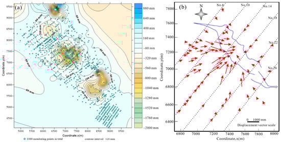
Figure 2.
Characteristics of vertical and horizontal displacement at the Jinchuan Nickel Mine: (a) Distribution of GPS monitoring points at Jinchuan Nickel Mine overlying a contour map of the vertical displacements recorded for October 2015, using May 2005 as a baseline. (b) Diagram of horizontal displacement vectors at mine field No.2 in October 2015, using May 2001 as a reference measure.
A positive vertical displacement value represents uplift events, while a negative value represents subsidence events. Subsidence or uplift events for a specific monitoring point can occur at any time. The horizontal and vertical displacement of a monitoring point over the monitoring period changed often, exhibiting stochastic fluctuation. As time progressed, displacements of various magnitudes occurred, giving rise to a cumulative settlement increase. The variation in displacements of the specific monitoring points was similar. This is because the variation in displacement is related to changes in the surrounding rock pressure and rock mass structure, as well as the shape, depth, intensity and scope of the mining. For instance, at minefield No.2, the extracted ore tonnage was 2.27 million tons in 2001 but reached 4.18 million tons in 2010. Ore production increased by 1.8 times from 2001 to 2010, while the corresponding maximum subsidence increased by 1.5 times, from 149 mm to 217 mm. During the whole monitoring period, the horizontal displacement rate and the cumulative horizontal displacements of the monitoring points increased year-by-year. By the end of 2015, the maximum horizontal displacement reached 1725 mm. The frequency of small and medium movement events at a given monitoring point was higher than for large movement events. Small, medium and large events have no specific quantitative values in this study but are used as relative terms only. Over the whole monitoring period, the recurrence time intervals in a certain displacement range were different too (Figure 3 and Figure 4). Sometimes, they were long and, sometimes, they were short. The recurrence time is the time interval between the beginning of two successive subsidence events that have the same magnitude.

Figure 3.
Mine subsidence time series of several monitoring points at the Jinchuan Nickel Mine: (a) monitoring point 2201, (b) monitoring point 2205, (c) monitoring point 6002, (d) monitoring point 6006.
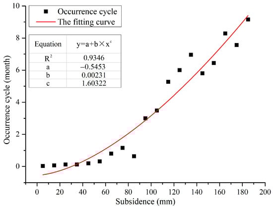
Figure 4.
Power-law relationship between the subsidence and its occurrence cycle.
A wide area was affected by vertical and horizontal displacements caused by ground movement. Three different subsidence troughs formed within the minefield (Figure 2a). All subsidence troughs were centered on the mined-out space. They progressively developed and expanded as mining depth increased. At mine field No.2, almost all horizontal displacement vectors point at the underground goaf, and the displacement value changes with the distance from the center of the ore body (Figure 2b). With the intensification of ground movement, more and more ground fissures have formed on the ground surface. In recent years, some large cracks have joined together, making the damage to the ground surface more serious.
It can be seen from Figure 3 that the vertical displacements of the monitoring points were different due to their distance from the ore body. Despite some of the monitored points far away from the mining area exhibiting irreversible, long-lasting movements, the points far from the mining area (e.g., 2201, 6002) were more stable than the points near the mining area (e.g., 2205, 6006). The displacements of monitoring points near the mining area were larger than monitoring points further from the mining area. The linear trend of the ground-movement time series near the mining area was clearer than the time series far away from the mining area.
3.2. Statistical Relationship between the Subsidence and Its Occurrence Cycle
Statistical analysis of 500 monitoring points showed that the surface subsidence value of the same monitoring point had the characteristics of being repeated and spaced. A deeper exploration of the relationship between the amount of subsidence and its occurrence cycle improve understanding of the potential time-domain characteristics of surface subsidence. Firstly, the subsidence value was divided into different ranges, and then the number of times N that a certain range of subsidence occurred at the 500 monitoring points in the whole monitoring period (174 months) was counted. Thus, the occurrence cycle T was calculated according to the formula T = 174/N (month), as shown in Table 1.

Table 1.
Subsidence occurrence cycle of 500 monitoring points.
Figure 4 shows the statistical results of the subsidence value and the occurrence cycle. It can be seen that the small-scale subsidence had a short period and high frequency, while the large-scale subsidence volume had a long period and low frequency. According to the fitting results, there was a power-law relationship between the amount of subsidence and its occurrence cycle.
3.3. Signal Analysis Methods and Results
3.3.1. Signal Analysis Methods
A time series is a set of observations arranged in chronological order. Time series can be divided into continuous time series and discrete time series. The time series studied in this paper is a type of discrete time series. If the future value of a time series can only be described by a probability distribution, then the time series is indecisive or just a statistical time series.
Time series can be analyzed in the time domain and frequency domain. To discern and analyze whether a periodicity in a ground movement time series exists, the signal processing method is an effective tool. The autocorrelation function can be used to check the periodicity and persistence of a time series [,]. The autocorrelation function of a time series determines the change in the linear correlation coefficient of the time series. The values of the autocorrelation coefficient, Rh, can be used to measure persistence. Positive and negative values of Rh indicate persistence and anti-persistence, respectively. For an uncorrelated time series, the value will be zero. If there is a periodic signal hidden in the time series, the autocorrelation function will have a sinusoidal shape, which can testify to the existence of periodicity []. For a discrete time series, the autocorrelation coefficient, Rh, can be calculated using the following formula:
N The number of values in the time series;
Yi The value of the time series at time ti;
The mean value of the time series;
K Time lag (k = 0, 1, 2, …).
Based on the assumption that sine and cosine waves with various frequencies constitute the time series, it can be analyzed in the frequency domain via the spectral analysis method. The self-affinity and fundamental frequency of the time series can also be studied via the spectral analysis method. According to several studies, the basic definition of a self-affine time series is that the power spectrum, (S(f)), of the time series has a power-law dependence on the frequency, (f) [,,], taking
where β is the power-spectral exponent. A great deal of information about s time series can be provided by the power spectrum. Variations in time series contain important interpretations for physical systems. These power variations in frequency can be revealed by the power spectrum. The power spectrum of a discrete time series can be calculated with the Fourier transform method.
Consider a discrete time series, yn, where i = 1,2,3, …, N and the total time interval is T. The total time interval is divided into N equal intervals of length δ, with δ = T/N. The Fourier transform result of the discrete time series [] is
The power spectrum of a discrete time series, yn, can be written as
The power spectrum of a time series is also related to the autocorrelation function [], which can also be calculated using the following formula:
Before carrying out a Fourier transform on a time series, the trend of the data should be taken into account. Removing the trend of a time series is always recommended. When the trend is removed, the mean of the time series’ data is equal to 0, and the variance is normalized to 1; thus, the Fourier coefficients and the slope of the power spectrum function will not be affected. However, care should be taken when detrending a time series since there are some controversies surrounding it. If a time series presents a distinct linear trend and the values are closely scattered around a straight line, then the linear trend can be safely removed. In contrast, if there is no clear linear trend, detrending the linear trend will change the statistical result of the slope of the power spectrum function [,]. For more details about Fourier transform and self-affine time series, several studies can be consulted [,].
The values of a time series can affect other values that are not only nearby in time, but also far away in time. If a time series exhibits persistence, the values within the time series are correlated, and the correlations can be strong, weak or nonexistent []. When the data are positively correlated, big values tend to follow. The correlations refer to the statistical dependence of neighbored values in the time series. When we analyze the correlations of values in a time series, two types of correlations are considered; one is short-range persistence, and the other is long-range persistence [,]. If a time series is short-range persistent, a number of preceding values influence the next value, and the persistence is characterized by an exponential decay. Conversely, long-range persistence is characterized by power-law decay, and almost all values in the time series are correlated with one another on a very large timescale [].
To quantify the temporal correlations and the strength of persistence in self-affine time series, the spectral exponents, β, must be analyzed []. The spectral exponent quantifies how variability is distributed across the frequency domain and is a measure of the strength of persistence or anti-persistence in a time series [,]. When β > 0, the time series is long-range persistent, and the correlations between neighbored values become stronger. If 0 < β < 1, the time series shows weak persistence, is stationary and both the mean and variance are constants. If β > 1, strong persistence exists in the time series, which is nonstationary with mean and variance changes in the recorded length []. If β = 0, the time series corresponds to white noise, and the correlations between the values are nonexistent [,]. A self-affine time series with β < 0 exhibits long-range anti-persistence.
The value of a spectral exponent, β, is the slope of the best-fit straight line to the power spectrum and frequency in a log–log plot. If the least-square method is applied to fit the logarithmized data, a higher exponent will, misleadingly, be obtained; the same problem will occur if we fit a power law to the data. When the general maximum likelihood method is used, this problem can generally be avoided. Thus, when determining the power spectral exponent of a ground-movement time series, the general maximum likelihood method is applied.
3.3.2. Autocorrelation Analysis Results of Ground Movement
In this study, the time series and autocorrelation plots for all the monitoring points were analyzed. We found that the characteristics of some time series were complex, having approximately sinusoidal shapes and linear trends. Some of the ground-movement time series contained clear long-term linear trends (e.g., 2206 and 6006 in Figure 3), which could influence the analysis results. To reduce error, a series should be linearly detrended. For example, Figure 5 shows the non-detrended and detrended time series and autocorrelation plots for the monitoring point 6001. The horizontal and vertical displacement time series and the autocorrelation plots all have approximately sinusoidal shapes, and the fluctuating forms are complicated. This indicates that a hidden complex periodicity exists in the time series. The autocorrelation coefficients of the horizontal and vertical displacements of the monitoring point 6001 centered between positive and negative 0.4.

Figure 5.
Non-detrended and detrended vertical and horizontal displacement time series and autocorrelation plots of the monitoring point 6001 at the Jinchuan Nickel Mine: (a) Horizontal displacement, (b) vertical displacement, (c) detrended horizontal displacement, (d) detrended vertical displacement, (e) autocorrelation plot of horizontal displacement, (f) autocorrelation plot of vertical displacement.
3.3.3. Spectral Analysis Results of Ground Movement
To study the ground-movement dynamics, self-affinity, fundamental frequency and persistence of the ground-movement events, the power spectra of the time series were analyzed; the timescale ranged from six months to 14.5 years. We performed a spectral analysis on the ground movement time series of 500 randomly distributed monitoring points. The time series data were plotted in double logarithmic plots; the vertical and horizontal coordinates were logarithms of the power spectrum, S(f), and the logarithms of frequency f, respectively.
The power spectrum of the horizontal and vertical displacements has a power-law dependence on frequency, with a linear decrease in the double logarithmic plot (Figure 6). This shows that a log–log linear relationship exists between the frequency and the corresponding power spectrum at any timescale. This relationship is best approximated by a power-law decay, S(f) ~.

Figure 6.
Power spectra of the horizontal and vertical displacement in the monitoring point 2207 at minefield No.2 and the monitoring point 2003 at minefield No.1 in log S(f)–log (f) and log S(f)–f plots: (a,b): power spectra of the horizontal and vertical displacement of the monitoring point 2207 in a log S(f)–log (f) plot; (c,d): power spectra of the horizontal and vertical displacement of the monitoring point 2207 in a log S(f)–f plot; (e,f): power spectra of the horizontal and vertical displacement of the monitoring point 2003 in a log S(f)–log (f) plot; (g,h): power spectra of the horizontal and vertical displacement of the monitoring point 2003 in a log S(f)–f plot.
We analyzed all the spectral exponents, β, and found that the exponents of vertical displacement ranged from 0.43 to 3.37, and most were between 1.11 and 2.96, with the mode and mean values being 1.51 and 1.79, respectively. As for horizontal displacement, the spectral exponents, β, ranged from 0.47 to 3.58, and most of them were between 1.22 and 3.18, with the mode and mean values being 2.76 and 2.05, respectively.
Furthermore, we found that the predominant frequencies of the horizontal and vertical displacements in minefields No.1 and No.2 were different (Figure 6). The predominant frequencies of horizontal and vertical displacements in minefield No.1 were 0.9558 and 0.9447, corresponding to approximately 1.1 months. At minefield No.2, the predominant frequencies were 0.7133 and 0.7573, corresponding to approximately 1.4 months.
4. Discussion
4.1. Self-Affinity, Long-Range Persistence and Scale-Invariance of Ground Movement
A spectral analysis of a regionally distributed, mining-induced ground-movement time series is presented, showing that the time series is universally self-affine and that the power spectrum has a power-law on frequency. Although several engineering geological conditions, including mining intensity, rock mass fracture, the geometry of the working face, etc., are different, the power spectra of different ground movement time series show the same power-law behavior. The power-law correlation between the power spectrum and the frequency also suggests that mining-induced ground movement is a type of noise. The spectral exponents, β, of horizontal and vertical displacement indicate the absence of any characteristic timescale in the power-law range.
Power-law behavior describes fractal or scale-invariant relationships, and it arises from scale-invariant processes []. Thus, the ground movement is scale-invariant in the timescale. The scaling behavior of the time series is closely linked to several features, such as long-range persistence and self-affinity, and these features are characterized by the fact that their power spectra show power-law behaviors []. The self-affinity also shows certain fractal characteristics, and, if the time series is scale-invariant, no characteristic timescale can be distinguished from either the whole or the parts of the series [].
Different from statistically self-similar fractals, self-affine fractals, which are statistically similar under anisotropic scaling are, by definition, generally anisotropic rather than isotropic []. Due to the complicated structure of the rock mass, the ground-movement system shows anisotropy; thus, we argue that the ground movement’s self-affine time series has the characteristic of scale invariance, confirming the anisotropy of the ground movement system. The scale invariance of the time series reflects the physical and dynamic mechanisms of ground-movement phenomena and is also helpful in gaining a better understanding of related mining-induced hazards.
A time series characterized by long-range persistence is referred to as a long-memory time series. As we found above, mining-induced ground movement is a self-affine time series. The exponent of vertical displacement ranged from 0.43 to 3.37, and the exponent of horizontal displacement ranged from 0.47 to 3.58. This indicates that the time series exhibited long-range persistence. The autocorrelation analysis results also confirmed that the ground-movement time series showed persistence. The spectral exponent also indicated that there was no characteristic timescale in the range of the power law. In other words, the long-range correlations between the time series values occurred over a large timescale. The long-range persistence indicated that almost all values in the time series were correlated with one another on a very large timescale [], contributing to the prediction of future values. In addition, long-range temporal correlations always exist in non-equilibrium systems [], which indicates that the mining-induced ground movement system was far from equilibrium.
4.2. The Periodicity and The Predictability of Mining-Induced Ground Movement
The change in the ground-movement time series shown in Figure 6 has a sinusoidal shape. This was obvious for all monitoring points. A sinusoidal shape also appears in the autocorrelation plots. A clear periodicity in the values of the horizontal and vertical displacements of all the monitoring points is indicated by the sinusoidal shape, which means that the fluctuations in the ground movement are likely characterized by a periodic signal.
The spectral analysis results of the data indicate that the ground movement of minefield No.1 has an approximately 1.1-month fundamental period, while the fundamental period of minefield No.2 is very close to 1.4 months. The predominant frequencies are different in different regions. As analyzed above, the displacements of different minefields are characterized by diverse hidden frequencies and periodicities, which may be directly related to mining history and mining methods. After about 30 years of open-pit mining, minefield No.1 completely converted to underground mining; the mining history and mining method are totally different from minefields No.2 and No.3. In minefields No.2 and No.3, the mining method was underground mining from the very beginning. Periodicity is a significant factor that helps us understand periodic patterns of mining-induced ground movement and discover the underlying periodical influence factors. For example, the ground-movement periodicity may be related to the periodical mining rate or the ore yield.
Among the many phenomena in earth sciences, there are several hazards, such as landslides, floods and earthquakes. These hazards kill many people every year, and lives may be saved if the hazards can be predicted in the short term. In statistical prediction, the increase in uncertainty needs to be considered. Power-law behaviors have a slow power-law decay at large scales, which means that the increase in uncertainty follows a negative power law rather than an exponential one. The power spectrum of a self-affine time series is a useful tool to evaluate event occurrences in the temporal domain, and a self-affine time series is likely to have sufficient memory for a scale-invariant signal and slow power-law decay [,]. This slow increase is positive for short-term statistical forecasts of occurrence rates []. Periodicity is undoubtedly a frequent phenomenon among all important movement patterns. Finding periodic behaviors is significant for understanding the underlying patterns of physical objects, predicting future movements and identifying abnormal phenomena. The mining-induced ground-movement time series exhibits long-range persistence, and long-range temporal correlations between movement values and periodicity also contribute to the short-term prediction of hazards.
4.3. Underlying Mechanism of Power-Law Behaviors
As discussed above, the power spectrum of the ground-movement time series displays power-law behavior across different timescales. This power law indicates that mining-induced ground movement is a type of f -β noise. f -β noise is a broader form of 1/f noise, which was put forward by Per Bak [,]. As a broader form of 1/f noise, f -β noise contains several special categories, including pink noise with β = 1, red noise with β = 2, black noise with β = 3 and other noises []. 1/f noise has been observed in many physical phenomena, and the power spectra of these phenomena display power-law behaviors [,].
Many researchers have argued that power-law behaviors are the consequence of SOC (self-organized criticality) [,,]. SOC was put forward to illustrate the evolution patterns and characteristics of nonlinear complex systems [,]. In a self-organized critical state, the size distribution of unstable events has a power-law distribution [,], which means that the emergence of scale-invariant structures can be a spatial fingerprint of SOC. The other self-organized critical behavior is 1/f noise [,], in which the power spectrum has a power-law dependence on frequency. 1/f noise, which is related to the occurrence of a self-organized critical state, is characterized by correlations extended over a wide range of timescales and indicates the underlying mechanism of self-organized critical systems [,,]. Self-organized criticality is considered scale-invariant; in particular, long-range correlations occur between different spatial and temporal scaling fields []. In a self-organized critical state, a frequency spectrum distribution, , can result from a power-law distribution over the lifetime of events: [,].
Over time, a self-organized process that is dynamic but far from equilibrium will develop into a self-organized critical state. When a system evolves into a self-organized critical state, a chain-reaction can be caused by minor events, and large events can be triggered []. During self-organization, interactions between a unit and its nearest neighbors often vary, and the combined effect of these interactions varies, too. Thus, these systems remain far from equilibrium and never develop into a stable state, although they may have stable statistical properties. In a self-organized criticality system, the “input” to a complex system is constant, whereas the “output” is a series of events or “avalanches” that follow power-law behavior []. Only when a system is open, nonlinear, far from equilibrium, and both robust and sensitive, can power-law behavior resulting from SOC be studied systematically.
In deforming systems, the deformed solids are nonlinear dynamic systems with self-organized criticality. Power laws can be used to describe features with long-range space–time correlations, such as the self-similarity of fractures, as well as damage accumulation over the entire hierarchy of scales. In particular, Makarov argued that the deformed medium should be considered a multiscale, nonlinear system to evaluate the possibility of mine roof collapses. Mining-induced ground-movement systems are open systems because both matter and energy are exchanged with regions outside the system. Surrounding rock stress fields, rock mass structures and other factors all change in time and space, while nonlinear interactions among them make the physical process of movement very complex and nonlinear. Although a local and temporary stable state may develop, the system is still far from equilibrium, reflecting such nonlinear interactions. In rock engineering, the failure or instability of a rock mass is mainly determined by excavation unloading and other environmental factors (e.g., water, temperature). Excavation causes the original stress balance of the rock mass to be disturbed, and stress redistribution occurs. Internal cracks accumulate and develop, eventually bringing about the failure of the rock mass. When new fractures occur in a rock element, other elements are affected as energy releases, triggering more fractures to develop. Randomly distributed fractures concentrate, forming a failure surface and leading to rock failure. Thus, small failure elements can cause a chain-reaction within the rock system. This process shows the sensitivity of the deforming system. On most occasions, the failure of a rock element does not immediately trigger a mine roof collapse or ground movement because of the robustness of the rock mass system. Although nonlinear interactions between the stress field, structural failure planes and rock blocks are extremely strong, the progressive increase in the system’s sensitivity can be restricted by overall rock mass stability, leading to robustness in the system.
As outlined above, mining-induced ground-movement systems have the characteristics of SOC. They can develop critical states through self-organized evolution, governed by power laws.
4.4. Influencing Factors of Power Spectral Exponents
The spectral exponents, β, of the horizontal and vertical displacements of ground-movement change over different locations. Other natural phenomena governed by power-law behavior also exhibit changes in their exponent values. Studies show that the distribution of surface displacements and fault geometry, as well as the correlations between them, may be related to the spatial and temporal power-law behavior of aseismic slips. The depth of soil deposits, soil density, shear modulus, corner frequency of the source and the high-frequency decay rate of acceleration are factors that control the spectral shape of ground motion []. Some researchers argue that the power-law exponents of landslides may vary with the underlying geology [,,]. Meanwhile, the retreat of cliffs or coastal bluffs is greatly dependent on the frequency of wave attacks at the cliff toe and rain intensity. These studies cause us to speculate that variation in the spectral exponent of ground movement is associated with variation in rock mass movement triggers.
The range of ground movement in the mine and the ground-movement magnitude are related to many rock mass movement triggers, including the mining history, mining area, mining rate, mining intensity, mining method, mining depth, ore yield, structural setting, host rock stress field, rock mass structure, rock mass fracture intensity, and the geometry of the working face, as well as the thickness and distribution of the overburden and topsoil. Underground mining is essentially an unloading process in which rock mass failure is characterized by several distinct deformation stages. These stages include crack initiation, crack propagation and coalescence. The distribution of unloading-induced cracks affects both the overlying rock mass’s geo-mechanical behavior and its stability, which, in turn, control the magnitude of ground movement. As rock mass movement triggers, both the unloading value and the unloading rate affect fissure development and the settlement of a mining-influenced system for a given region over a given timescale. The relationship between joint movement and mining-induced ground movement has been studied in detail. It has been shown that the broken expansion coefficients are positively correlated with the fractal dimension of a rock’s fractures [,]. During the evolution of a fracture network, new fractures are added to the established network, making it more complex. In this way, the fractal dimension of the network increases over time []. Although the fractal distribution of a rock mass’s fracture length and spacing has been studied [], the association between the spectral exponents and the fractal distribution of failure planes remains speculative. In addition, tectonic stress also controls ground movement. We found that two subsiding centers could occur within some subsidence troughs; this phenomenon is related to the high level of tectonic stress within the study area []. Rock mass deformation and damage are closely related to the magnitudes and orientations of the maximum and minimum principal stresses. The existence of high-level tectonic stress alleviates the magnitude of vertical subsidence and promotes the horizontal deformation of the ground [].
In different positions in a mining-influenced area, the factors discussed above often vary. During mining, rock mass movement triggers change over time and location. Therefore, changes in both the magnitude and frequency of ground-movement events cause the spectral exponents to change based on location.
5. Conclusions
(1) The mining-induced ground movements of 500 randomly selected GPS monitoring points were analyzed. We found that points far from the ore body were more stable than those near the ore body, and their linear trend in the time series was more obvious. Over the whole monitoring period, the surface subsidence of the same monitoring points had the characteristics of repetition and spacing. The spectral exponents of the horizontal and vertical displacements ranged from 0.47 to 3.58 and from 0.43 to 3.37, with mean values of 2.05 and 1.79, respectively. The ground movement of minefields No.1 and No.2 had 1.1-month and 1.4-month fundamental periods, respectively.
(2) The power spectra of ground-movement time series showed a power-law dependence on frequency. This indicates that the time series is self-affine on different timescales and is a type of noise. The power-law behavior of the time series may be related to the self-organized criticality of the ground-movement system, and it reflects the scale-invariance of the ground-movement system in the timescale. The variation in the value of the spectral exponent may be associated with rock-movement triggers.
(3) A hidden fundamental period exists in the ground-movement time series, the correlations between ground-movement values within the time series are strong, and long-range persistence occurs over a large timescale. Together with the power-law behavior, long-range persistence and periodicity benefit the short-range prediction of mining-induced ground movements. These results provide a basis for studying the underlying patterns of mining-induced ground movements in more detail.
Author Contributions
Data curation, G.L.; formal analysis, X.H. and J.G.; methodology, G.L. and X.H.; software, G.L.; writing—original draft, G.L.; writing—review and editing, G.L., J.G. and F.M.; experiments, G.L. and J.G. All authors have read and agreed to the published version of the manuscript.
Funding
This research was supported by the National Natural Science Foundation of China (Grant Nos. 42072305 and 41831293).
Data Availability Statement
Not applicable.
Acknowledgments
The authors would like to express their sincere gratitude to Jinchuan Nickel Mine for their data support. In addition, the authors are grateful to assigned editors and anonymous reviewers for their enthusiastic help and valuable comments which have greatly improved this paper.
Conflicts of Interest
The authors declare that they have no conflict of interest regarding this study. We declare that we do not have any commercial or associative interests that represent a conflict of interest in connection with the paper submitted.
References
- Ma, D.; Zhao, S. Quantitative Analysis of Land Subsidence and Its Effect on Vegetation in Xishan Coalfield of Shanxi Province. ISPRS Int. J. Geo-Inf. 2022, 11, 154. [Google Scholar] [CrossRef]
- Ma, F.S.; Zhao, H.J.; Yuan, R.M.; Guo, J. Ground movement resulting from underground backfill mining in a nickel mine (Gansu Province, China). Nat. Hazards 2015, 77, 1475–1490. [Google Scholar] [CrossRef]
- Hu, W.; Wu, L.; Zhang, W.; Liu, B.; Xu, J. Ground Deformation Detection Using China’s ZY-3 Stereo Imagery in an Opencast Mining Area. ISPRS Int. J. Geo-Inf. 2017, 6, 361. [Google Scholar] [CrossRef]
- Zhao, H.J.; Ma, F.S.; Xu, J.M.; Guo, J. In situ stress field inversion and its application in mining-induced rock mass movement. Int. J. Rock Mech. Min. Sci. 2012, 53, 120–128. [Google Scholar] [CrossRef]
- Álvarez-Fernández, M.I.; González-Nicieza, C.; Menéndez-Díaz, A.; Álvarez-Vigil, A.E. Generalization of the n–k influence function to predict mining subsidence. Eng. Geol. 2005, 80, 1–36. [Google Scholar] [CrossRef]
- Díaz-Fernández, M.E.; Álvarez-Fernández, M.I.; Álvarez-Vigil, A.E. Computation of influence functions for automatic mining subsidence prediction. Comput. Geosci. 2010, 14, 83–103. [Google Scholar] [CrossRef]
- Li, G.; Wang, Z.; Ma, F.; Guo, J.; Liu, J.; Song, Y. A case study on deformation failure characteristics of overlying strata and critical mining upper limit in submarine mining. Water 2022, 14, 2465. [Google Scholar] [CrossRef]
- Song, J.; Han, C.; Ping, L.; Zhang, J.; Liu, D.; Jiang, M.; Zheng, L.; Zhang, J.; Song, J. Quantitative prediction of mining subsidence and its impact on the environment. Int. J. Min. Sci. Technol. 2012, 22, 69–73. [Google Scholar]
- Yushin, V.I.; Geza, N.I.; Yushkin, V.F.; Polozov, S.S. Measurement of rock movement under blasting in surface mines. J. Min. Sci. 2010, 46, 516–524. [Google Scholar] [CrossRef]
- Yu, G. Application of nonlinear seience in the mining subsidence. J. Fuxing Min. Inst. (Nat. Sci.) 1997, 16, 285–288. [Google Scholar]
- Figueirêdo, P.H.; Moret, M.A.; Pascutti, P.G.; Nogueira, E., Jr.; Coutinho, S. Self-affine analysis of protein energy. Phys. A Stat. Mech. Its Appl. 2010, 389, 2682–2686. [Google Scholar] [CrossRef]
- Suleymanov, A.A.; Abbasov, A.A.; Ismaylov, A.J. Fractal analysis of time series in oil and gas production. Chaos Solitons Fractals 2009, 41, 2474–2483. [Google Scholar] [CrossRef]
- Mandelbrot, B.B.; Van Ness, J.W. Fractional Brownian motions, fractional noises and applications. Siam Rev. 1968, 10, 422–437. [Google Scholar] [CrossRef]
- Malamud, B.D.; Turcotte, D.L. Self-affine time series: I. Generation and analyses. Adv. Geophys. 1999, 40, 1–90. [Google Scholar]
- Williams, Z.C.; Pelletier, J.D. Self-affinity and surface-area-dependent fluctuations of lake-level time series. Water Resour. Res. 2015, 51, 7258–7269. [Google Scholar] [CrossRef]
- Dussauge, C.; Grasso, J.R.; Helmstetter, A. Statistical analysis of rockfall volume distributions: Implications for rockfall dynamics. J. Geophys. Res. Solid Earth 2003, 108, 12–19. [Google Scholar] [CrossRef]
- Malamud, B.D.; Turcotte, D.L. Self-organized criticality applied to natural hazards. Nat. Hazards 1999, 20, 93–116. [Google Scholar] [CrossRef]
- Malamud, B.D.; Turcotte, D.L. The applicability of power-law frequency statistics to floods. J. Hydrol. 2006, 322, 168–180. [Google Scholar] [CrossRef]
- Pandey, G.; Lovejoy, S.; Schertzer, D. Multifractal analysis of daily river flows including extremes for basins of five to two million square kilometres, one day to 75 years. J. Hydrol. 1998, 208, 62–81. [Google Scholar] [CrossRef]
- Teixeira, S.B. Slope mass movements on rocky sea-cliffs: A power-law distributed natural hazard on the Barlavento Coast, Algarve, Portugal. Cont. Shelf Res. 2006, 26, 1077–1091. [Google Scholar] [CrossRef]
- Witt, A.; Malamud, B.D. Quantification of Long-Range Persistence in Geophysical Time Series: Conventional and Benchmark-Based Improvement Techniques. Surv. Geophys. 2013, 34, 541–651. [Google Scholar] [CrossRef]
- Crosby, N. Frequency distributions: From the sun to the earth. Nonlinear Process. Geophys. 2011, 18, 791–805. [Google Scholar] [CrossRef]
- Hergarten, S.; Neugebauer, H.J. Self-organized criticality in a landslide model. Geophys. Res. Lett. 1998, 25, 801–804. [Google Scholar] [CrossRef]
- Palus, M.; Novotna, D.; Zvelebil, J. Fractal rock slope dynamics anticipating a collapse. Phys. Rev. E Stat. Nonlinear Soft Matter Phys. 2004, 70, 036212. [Google Scholar] [CrossRef]
- Bak, P.; Tang, C.; Wiesenfeld, K. Self-organized criticality: An explanation of the 1/f noise. Phys. Rev. Lett. 1987, 59, 381–394. [Google Scholar] [CrossRef]
- Li, G.; Ma, F.; Guo, J.; Zhao, H. Experimental research on deformation failure process of roadway tunnel in fractured rock mass induced by mining excavation. Environ. Earth Sci. 2022, 81, 243. [Google Scholar] [CrossRef]
- Li, G.; Ma, F.; Guo, J.; Zhao, H.; Liu, G. Study on deformation failure mechanism and support technology of deep soft rock roadway. Eng. Geol. 2020, 264, 105262. [Google Scholar] [CrossRef]
- Li, G.; Ma, F.; Guo, J.; Zhao, H. Deformation Characteristics and Control Method of Kilometer-Depth Roadways in a Nickel Mine: A Case Study. Appl. Sci. 2020, 10, 3937. [Google Scholar] [CrossRef]
- Li, G.; Ma, F.; Guo, J.; Zhao, H. Case Study of Roadway Deformation Failure Mechanisms: Field Investigation and Numerical Simulation. Energies 2021, 14, 1032. [Google Scholar] [CrossRef]
- Zhao, H.J.; Ma, F.S.; Zhang, Y.M.; Guo, J. Monitoring and Analysis of the Mining-Induced Ground Movement in the Longshou Mine, China. Rock Mech. Rock Eng. 2013, 46, 207–211. [Google Scholar] [CrossRef]
- Hui, X.; Ma, F.; Guo, J.; Xu, J. Power-law correlations of mine subsidence for a metal mine in China. Environ. Geotech. 2021, 8, 559–570. [Google Scholar] [CrossRef]
- Li, G.; Wan, Y.; Guo, J.; Ma, F.; Zhao, H.; Li, Z. A Case Study on Ground Subsidence and Backfill Deformation Induced by Multi-Stage Filling Mining in a Steeply Inclined Ore Body. Remote Sens. 2022, 14, 4555. [Google Scholar] [CrossRef]
- Zhao, H.J.; Ma, F.S.; Zhang, Y.M.; Guo, J. Monitoring and mechanisms of ground deformation and ground fissures induced by cut-and-fill mining in the Jinchuan Mine 2, China. Environ. Earth Sci. 2013, 68, 1903–1911. [Google Scholar] [CrossRef]
- Hui, X.; Ma, F.; Zhao, H.; Xu, J. Monitoring and statistical analysis of mine subsidence at three metal mines in China. Bull. Eng. Geol. Environ. 2019, 78, 3983–4001. [Google Scholar] [CrossRef]
- Zhao, H.J.; Ma, F.S.; Zhang, Y.M.; Guo, J. Monitoring and assessment of mining subsidence in a metal mine in China. Environ. Eng. Manag. J. 2014, 13, 3015–3024. [Google Scholar] [CrossRef]
- Box, G.E.P.; Jenkins, G.M.; Reinsel, G.C. Time Series Analysis: Forecasting and Control; Holden-Day: Oakland, CA, USA, 1976; Volume 37, pp. 238–242. [Google Scholar]
- Priest, S.; Hudson, J. Discontinuity spacings in rock. Int. J. Rock Mech. Min. Sci. Geomech. Abstr. 1976, 13, 135–148. [Google Scholar] [CrossRef]
- Pelletier, J.D.; Turcotte, D.L. Self-Affine Time Series: II. Applications and Models. Adv. Geophys. 1999, 40, 91–166. [Google Scholar]
- Turcotte, D.L.; Brown, S.R. Fractals and Chaos in Geology and Geophysics, 2nd ed.; Cambridge University Press: Cambridge, UK, 1997. [Google Scholar]
- Glosup, J. Statistics for long-memory processes. Technometrics 1994, 39, 105–106. [Google Scholar] [CrossRef]
- Beran, J. Statistics for Long-Memory Processes; Chapman & Hall/CRC: New York, NY, USA, 1994. [Google Scholar]
- Turcotte, D.L. The relationship of fractals in geophysics to “the new science”. Chaos Solitons Fractals 2004, 19, 255–258. [Google Scholar] [CrossRef]
- Zaourar, N.; Hamoudi, M.; Mandea, M.; Balasis, G.; Holschneider, M. Wavelet-based multiscale analysis of geomagnetic disturbance. Earth Planets Space 2013, 65, 1525–1540. [Google Scholar] [CrossRef]
- Ghil, M.; Yiou, P.; Hallegatte, S.; Malamud, B.D.; Naveau, P.; Soloviev, A.; Friederichs, P.; Keilis-Borok, V.; Kondrashov, D.; Kossobokov, V.; et al. Extreme events: Dynamics, statistics and prediction. Nonlinear Process. Geophys. 2011, 18, 295–350. [Google Scholar] [CrossRef]
- McAteer, R.T.; Aschwanden, M.J.; Dimitropoulou, M.; Georgoulis, M.K.; Pruessner, G.; Morales, L.; Ireland, J.; Abramenko, V. 25 Years of Self-organized Criticality: Numerical Detection Methods. Space Sci. Rev. 2016, 198, 217–266. [Google Scholar] [CrossRef]
- Corona, O.L.; Padilla, P.; Escolero, O.; Frank, A.; Fossion, R. Lévy flights, 1/f noise and self organized criticality in a traveling agent model. J. Mod. Phys. 2013, 4, 337–343. [Google Scholar] [CrossRef]
- Yao, L. Self-organized criticality and its application in the slope disasters under gravity. Sci. China Ser. E Technol. Sci. 2003, 46, 20–30. [Google Scholar] [CrossRef]
- Pruessner, G. Self-Organised Criticality: Theory, Models and Characterization; Cambridge University Press: Cambridge, UK, 2012. [Google Scholar]
- Bak, P.; Tang, C.; Wiesenfeld, K. Self-Organized Criticality. Phys. Rev. A 1988, 38, 364–374. [Google Scholar] [CrossRef] [PubMed]
- Iwahashi, J.; Watanabe, S.; Furuya, T. Mean slope-angle frequency distribution and size frequency distribution of landslide masses in Higashikubiki area, Japan. Geomorphology 2003, 50, 349–364. [Google Scholar] [CrossRef]
- Stark, C.P.; Hovius, N. The characterization of landslide size distributions. Geophys. Res. Lett. 2001, 28, 1091–1094. [Google Scholar] [CrossRef]
- Mandelbrot, B.B.; Pignoni, R. The Fractal Geometry of Nature; WH freeman: New York, NY, USA, 1983. [Google Scholar]
- Bak, P. How nature works: The science of self-organized criticality. Nature 1996, 383, 772–773. [Google Scholar]
- Loh, C.H.; Su, G.W.; Yeh, C.S. Development of stochastic ground movement-study on smart-1 array data. Soil Dyn. Earthq. Eng. 1989, 8, 22–31. [Google Scholar] [CrossRef]
- Frattini, P.; Crosta, G.B. The role of material properties and landscape morphology on landslide size distributions. Earth Planet. Sci. Lett. 2013, 361, 310–319. [Google Scholar] [CrossRef]
- Guzzetti, F.; Ardizzone, F.; Cardinali, M.; Galli, M.; Reichenbach, P.; Rossi, M. Distribution of landslides in the Upper Tiber River basin, central Italy. Geomorphology 2008, 96, 105–122. [Google Scholar] [CrossRef]
- Swift, G. Relationship between joint movement and mining subsidence. Bull. Eng. Geol. Environ. 2014, 73, 163–176. [Google Scholar] [CrossRef]
- Zhang, Y.; Jin, Z.; Liu, X. Testing study on fractal correlation law of cracks in mined rock masses. Chin. J. Rock Mech. Eng. 2004, 23, 3426–3429. [Google Scholar]
Publisher’s Note: MDPI stays neutral with regard to jurisdictional claims in published maps and institutional affiliations. |
© 2022 by the authors. Licensee MDPI, Basel, Switzerland. This article is an open access article distributed under the terms and conditions of the Creative Commons Attribution (CC BY) license (https://creativecommons.org/licenses/by/4.0/).