Abstract
Forest logging detection is important for sustainable forest management. The traditional optical satellite images with visible and near-infrared bands showed the ability to identify intensive timber logging. However, less intensive logging is still difficult to detect with coarse spatial resolution such as Landsat or high spatial resolution in fewer spectral bands. Although more high-resolution remote sensing images containing richer spectral bands can be easily obtained nowadays, the questions of whether they facilitate the detection of logging patterns and which spectral bands are more effective in detecting logging patterns, especially in selective logging, remain unresolved. Therefore, this paper aims to evaluate the combinations of visible, near-infrared, red-edge, and short-wave infrared bands in detecting three different logging intensity patterns, including unlogged (control check, CK), selective logging (SL), and clear-cutting (CC), in north subtropical plantation forests with the random forest algorithm using Sentinel-2 multispectral imagery. This study aims to explore the recognition performance of different combinations of spectral bands (visual (VIS) and near-infrared bands (NIR), VIS, NIR combined with red-edge, VIS, NIR combined with short-wave infrared bands (SWIR), and full-spectrum bands combined with VIS, NIR, red edge and SWIR) and to determine the best spectral variables to be used for identifying logging patterns, especially in SL. The study was conducted in Taizishan in Hubei province, China. A total of 213 subcompartments of different logging patterns were collected and the random forest algorithm was used to classify logging patterns. The results showed that full-spectrum bands which contain the red-edge and short-wave infrared bands improve the ability of conventional optical satellites to monitor forest logging patterns and can achieve an overall accuracy of 85%, especially for SL which can achieve 79% and 64% for precision and recall accuracy, respectively. The red-edge band (698–713 nm, B5 in Sentinel-2), short-wave infrared band (2100–2280 nm, B12 in Sentinel-2), and associated vegetation indices (NBR, NDre2, and NDre1) enhance the sensitivity of the spectral information to logging patterns, especially for the SL pattern, and the precision and recall accuracy can improve by 10% and 6%, respectively. Meanwhile, both clear-cutting and unlogged patterns could be well-classified whether adding a red-edge or SWIR band or both in VIS and NIR bands; the best precision and recall accuracies for clear-cutting were enhanced to 97%, 95% and 81%, 91% for unlogged, respectively. Our results demonstrate that the optical images have the potential ability to detect logging patterns especially for the clear-cutting and unlogged patterns, and the selective logging detection accuracy can be improved by adding red-edge and short-wave infrared spectral bands.
1. Introduction
Forests are the main component of the earth’s terrestrial ecosystem and play an irreplaceable role in water circulation, climate regulation, biodiversity, and carbon fixation functions [1,2]. Logging, such as selective logging, salvage logging, or clear-cutting, is the main approach for forest management, especially for a plantation forest. Proper logging patterns can improve the growing environment of trees and reduce the risk of pests and diseases, which helps to promote sustainable forest management. However, due to illegal logging or nonproper logging, which results in forests’ loss of diversity and carbon, it is very important to detect and monitor forest logging, which can help the administrators to find the forest changes after logging throughout the time range and understand the forest cover resistance, vegetation restoration patterns, the dynamic of the carbon budget, etc.
Optical satellite images with multispectral bands are commonly used in forest change detection. These conventional multispectral optical images show good results in land cover change or forest clear-cutting detecting. For example, MODIS-NDVI time series are able to detect deforestation within coniferous forests at a large scale and thus reflect historical forest health changes [3]. An object-oriented approach based on Landsat TM imagery can generate national-scale annual forest cover change distributions [4]. Landsat 8 fused with Gaofen-1 multispectral images and MOD13Q1 data can effectively estimate urban vegetation cover using time-mixing analysis [5]. These studies showed the potential ability of visible and near-infrared bands in detecting land cover or land cover change.
Furthermore, along with the development of remote sensing sensor technology, remote sensing images have contained richer spectral bands than conventional bands in recent years. The red-edge bands and short-wave infrared bands, which were widely used in vegetation detecting in situ, were gradually added to the satellite image bands. For example, WorldView-3 contains a red-edge band whose mean value plays an important role in the classification of forest resources using object-facing methods in conjunction with random forests [6]. Sentinel-2 has four unique red-edge bands and two short-wave infrared bands, which were widely used in forest detection. Moreover, the chlorophyll index calculated using its red-edge reflectance can monitor forest decline status [7]. Using its short-wave infrared bands to calculate the dNBR (differenced normalized burn ratio) and combining it with the maximum interclass variance algorithm, the location and area of forest fire areas with different degrees of burn can be determined [8]. The Gaofen-6 satellite, which launched in 2018, contains two new red-edge bands and near-infrared bands, respectively, and was widely used in forest dynamic detection [9,10]. The research which used these images have shown that containing more bands in images, especially red-edge bands, has a positive effect on tree species classifying and forest biochemical or physical parameter inversion [11,12,13].
In the forest logging detection field, it is hard work to detect the logging pattern with conventional multispectral optical images. Considering the logging intensity, the logging pattern is classified as selective logging and clear-cutting. The differences in the spectral characteristics in satellite images of forests before and after logging are not always significant. Regarding clear-cut patterns, studies reached better results when using only visible and near-infrared spectral bands. In contrast, forest selective logging, which is considered as a key factor in forest degradation and disturbance, did not perform well when detecting with optical data images. A high spatial resolution could help to improve the detecting accuracy, such as IKONOS and RapidEye [14,15]. However, it is costly to use these high-resolution imageries. Another way to improve the accuracy of detecting a selective logging pattern is to use time-series images for free, such as the Landsat system [16,17], which was commonly used in tropical forest disturbance mapping. Due to a relatively low resolution of 30 m, Landsat images cannot detect forest disturbances with less than 25% of the forest window within a single pixel [15]. Furthermore, it is difficult to obtain usable images on time due to the limitation of revisit cycles and cloudy images.
Due to the ability of LiDAR data to reflect the vertical structure of a forest, the penetrating nature of SAR to image in all weather, and the hyper-high spatial resolution of digital aerial photography, many studies exploring the potential of these data for monitoring selective logging in forests have had some success, but these studies are still limited by data availability and timeliness [18,19,20]. LiDAR data add uncertainty to logging identification, such as differences in the acquisition characteristics of multiperiod LiDAR data, limited flight areas, and limited accuracy of ground position and elevation if forest cover is high [21,22]. SAR data also suffer from high prices and speckle noise [23,24]. Digital aerial photography technology has similar problems to LiDAR, with complex acquisition and processing and low temporal resolution [25]. Therefore, free optical satellite imagery with multiple spectral bands remains the first choice for logging monitoring, with its advantages of continuity, stability, high positioning quality, and large area accessibility [26,27,28].
The Sentinel-2 satellite equipped with an optoelectronic multispectral sensor is another free data source, which can achieve a revisit period of 5 days by two polar-orbiting satellites placed in the same sun-synchronous orbit, phased at 180 to each other. The data can be publicly accessible and have a resolution of 10 to 20 m in visible, near-infrared, and short-wave infrared spectral zones [29]. In addition, Sentinel-2 images contain 13 spectral channels, especially in red-edge bands, which ensures the capture of differences in vegetation state changes. Therefore, the potential of different band combinations of Sentinel-2 for forest disturbance assessment remains to be further evaluated [30].
Considering there is a large amount of plantation forest in the north subtropical zone, we conducted this study to explore the capability of different optical spectral band combinations in Sentinel-2 images to identify plantation forest logging pattern. The aims were to find: (1) how optical bands with different combinations from low-cost satellite imagery influence the logging pattern detection; (2) which bands are more sensitive to the detecting logging patterns, especially selective logging; (3) how to promote the selecting logging pattern detecting with optical imagery containing red-edge and short-wave infrared bands.
2. Materials and Methods
2.1. Study Area and Samples
The study area was located in the Taizishan Forestry Administration Bureau in the southwestern part of Jingshan County, Hubei Province (Figure 1). It is a typical hilly landscape with an elevation between 40.3 m and 467.4 m, which is located in the transition zone from the remnants of the Dahongshan Mountains to the Jianghan Plain. The vegetation zone of the study area is a subtropical evergreen broad-leaved forest with high forest cover.
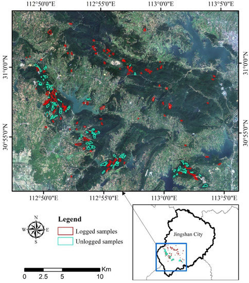
Figure 1.
The location of study areas which contained the logged and unlogged subcompartments.
The logging samples were collected from the local forest administrator, including 122 subcompartments. Subcompartments are the basic units of forest resource management, which are the forest stands with essentially the same internal characteristics such as tree species, structure, stand age, etc., and perform obviously different to outer stands. The logging samples were logged in the growing seasons (May–September) from 2016 to 2018. The 91 unlogged samples were randomly selected from the other subcompartments near the logging samples. The logging samples contained dominant tree species, logging method, logging volume, the total volume of the subcompartment, and the starting and ending time for each logging. The distribution of the logging and unlogged subcompartments can be seen in Figure 1.
2.2. Remote Sensing Data and Preprocessing
Sentinel-2 images were downloaded from the Copernicus Open Access Center. The band parameters are shown in Table 1. The images used in the research were selected considering the following reasons: (1) cloud-free images of the sample area; (2) as close as possible to the logging activities ceased; in this research, the mean time lag was 10 days and the maximum was 81 days due to the cloudy images. We used the visible, near-infrared, red-edge, and short-wave infrared spectral bands except band 1, band 9, and band 10 in this paper due to the low spatial resolution. The specific image time and the number of samples are shown in Table 2. Image preprocessing was carried out using SNAP software: (1) radiometric calibration; (2) atmospheric correction; (3) resampling to 10 m resolution.

Table 1.
Sentinel-2 band information.
Table 2.
Image date and number of samples.
2.3. Classification of Logging Patterns
In this study, the ratio of logging volume and total volume of the subcompartment was used to express the logging intensity (LI) (seen in Equation (1)). Based on the logging intensity, the logging samples were divided into selective logging (SL) and clear-cutting (CC) based on the distribution of the number of samples. The threshold to distinguish logging patterns was set to 30% according to the national forest conservation and logging specification [31]. There were three logging patterns, including unlogged which was defined as a control check (CK). Figure 2 illustrates the different logging patterns in the RGB images and Figure 3 illustrates the photos at the time of the selective logging and 2 weeks later. The number of samples and the range of logging intensity values are shown in Table 3.
Here, lv denotes the logging volume; sv denotes the total volume of the subcompartment.
Table 3.
The number of samples and the value range of each logging pattern.
Table 3.
The number of samples and the value range of each logging pattern.
| Logging Pattern | Number of Samples | Intensity Value Range | (Pre-Logging) Volume Per Hectare (m3/ha) | ||
|---|---|---|---|---|---|
| Range | Mean | SD | |||
| CK | 91 | 0% | 5.8~298.4 | 101.9 | 42.3 |
| SL | 59 | <30% | 42.8~274.6 | 138.2 | 54.7 |
| CC | 63 | 100% | 15.86~160.13 | 81.35 | 32.07 |
Notes: CK, SL, and CC indicate unlogged, selective logging, and clear-cutting, respectively.

Figure 2.
Different logging patterns in the RGB images.

Figure 3.
The photos at the time of selective logging and 2 weeks later. The left photo is the selective logging stand with 23.5% logging intensity. The right photo is two weeks after logging, in which one can find shrub and herbaceous plant recovery.
2.4. Feature Extraction for Logging Patterns Monitoring
In order to distinguish the logging pattern for each subcompartment, we extracted the averaged feature from images at the subcompartment boundary extent. The vegetation index and texture features were the commonly used features in the optical image, which showed good performance in forest disturbance detecting [32].
For the Sentinel-2 scenes given in Table 2, we extracted these vegetation indices to character the canopy status, including normalized difference vegetation index (NDVI), normalized burn ratio (NBR), green normalized difference vegetation index (GNDVI), ratio vegetation index (SR), and difference vegetation index (DVI) [33]. Among them, NBR applies near-infrared and short-wave infrared bands and is commonly used to detect the signal components of bare soil or nonphotosynthetic vegetation within the tropical rainforest canopy [34].
Since the red-edge bands are closely related to vegetation chlorophyll concentration [35], and the vegetation index calculated with the red-edge bands can reduce saturation compared to the traditional red-band vegetation index [36], the red-edge bands and related vegetation indices have been widely used in the fields of leaf area index estimation, biomass inversion, and forest fire disturbance monitoring [37,38,39]. As logging disturbance is similar to forest fire disturbance, which also influences the vegetation’s physical and chemical parameters such as the leaf area index and the chlorophyll content of leaves, the red-edge vegetation indices were calculated as part of the input feature set in this study. They include the normalized difference vegetation index with red-edge 1 (NDVIre1n), normalized difference vegetation index with red-edge 3 (NDVIre3n), chlorophyll index red-edge (CIre), normalized difference with red-edge 1 (NDre1), and normalized difference with red-edge 2 (NDre2) [40].
In addition, it was shown that texture measures such as contrast, variance, homogeneity, and entropy are associated with patch edge features, while mean, dissimilarity, angular second moment, and correlation are associated with tiny irregular variations within continuous regions such as forests [41]. The above eight texture feature values were calculated based on the first principal component (PCA) using a gray-level co-occurrence matrix to provide information on the local surrounding relationships of each pixel. The PCA transformation works on the 10 surface reflectance bands on Sentinel-2 which were introduced in Section 2.2. The cumulative contribution of the first principal component for each scene is more than 80%. The window size of the texture features is 7×7 and the gray level was set to 64 according to the reference of Jian and Hethcoat et al., which indicated that this window size is best for the forest parameter inversion on meter-level spatial-resolution remote sensing images [42,43]
Each feature set includes 28 components: 10 surface reflectance, 10 vegetation indices, and 8 texture features. Table 4 describes the various features and their expressions in detail.
Table 4.
The feature set description for modeling logging pattern classification.
2.5. Experimental Program Design
In order to test the effect of optical bands on logging pattern classification and select the best sensitive bands in logging detecting, we designed four cases in this study: (1) conventional optical bands only containing visual bands (VIS) and near-infrared bands (NIR); (2) conventional bands and red-edge bands (Red-edge); (3) conventional bands and short-wave infrared bands (SWIR); and (4) full-spectrum bands including conventional bands, red-edge bands, and short-wave infrared bands. The specific features included in these four cases are shown in the following table (Table 5).
Table 5.
Experimental program design.
2.6. Logging Patterns’ Identification Based on a Random Forest Algorithm
This study used the random forest classifier function inside the Python program Scikit-learn library to build a random forest (RF) model. RF is an aggregation algorithm derived from a decision tree (CART) [45], and unlike a single decision tree, the RF model uses multiple independent decision trees that can be used for problems such as classification and regression [46]. This study used its classification algorithm. The n_estimators and max_features are the main parameters of the algorithm. The former indicates the number of subtrees created before prediction using the maximum number of votes or the mean. The n_estimators was set to 300 by hyperparameter optimization. The parameter max_features indicates the number of features in the selected subfeature set. This study used the default method, the square root of the total number of features, and rounded off. The ranking of feature importance was performed according to the Gini index. A smaller Gini value indicates a higher purity of the dataset and higher importance of the variable [47].
2.7. Accuracy Assessment
Due to the small amount of data in the sample set, this study used the leave-one-out method for cross-validation to make full use of the limited data. This method can minimize the random error caused by assigning training and testing samples, thus preventing overfitting and determining the best model parameters [48]. The confusion matrix was used to calculate the accuracy metrics. The overall accuracy (Acc), kappa coefficient (Ka), F1-score, recall, and precision were calculated to evaluate the accuracy of the model. The formulas for the calculation of the indicators were as follows.
Acc = (TP + TN)/(TP + TN + FP + FN)
Kappa = (Acc − P_e)/(1 − P_e)
P_e = (P×P′ + N×N′)/(P + N)^2
P = TP + FN
P′ = TP + FP
N = FP + TN
N′ = FN + TN
Precision = TP/(TP + FP)
Recall = TP/(TP + FN)
F1_score = (2 × Precision × Recall)/(Precision + Recall)
TP denotes the number of positive classes predicted as positive classes; FP denotes the number of negative classes predicted as positive classes; TN denotes the number of negative classes predicted as negative classes; and FN denotes the number of positive classes predicted as negative classes.
3. Results
3.1. Evaluation of the Accuracy of Different Band Combinations
From the logging pattern identification results at different band combinations (Table 6), we found that full-spectrum bands (case 4) had the best results with an overall accuracy and kappa coefficient of 85% and 77%, respectively. Compared with case 1 with only VIS and NIR bands, the overall accuracy and kappa coefficient were improved by 5% and 8%, respectively. Case 2 and case 3, which added the red-edge bands and SWIR bands to the VIS and NIR bands, respectively, had relatively better identification results compared with case 1, both with an overall classification accuracy of 84% and kappa coefficients of 75% and 74%, respectively. The accuracy improved by 4% and the kappa coefficients improved by 6% and 5%, respectively, compared with case 1. The results show that based on VIS and NIR band data, adding either the red-edge bands or the SWIR bands can substantially improve the accuracy of logging patterns’ detection, and the detecting effect will achieve the best results when they are simultaneously added.
Table 6.
Accuracy comparison of classification results.
In terms of logging pattern, the highest recognition accuracy was found for clear-cutting, with recall, precision, and F1-scores around 95%, followed by unlogged types (76–91%), and the lowest recognition accuracy was found for selective logging (58–79%). For clear-cutting, adding more bands only improved the recognition accuracy by about 2%. For unlogged and selective logging, adding red-edge bands or adding SWIR bands improved the recognition accuracy to a limited extent, which could achieve a 2–4% improvement for the unlogged pattern and 3–6% for the selective logging pattern. In contrast, adding red-edge and SWIR together can maximize the recognition accuracy. The full-spectrum images can specifically improve the recognition accuracy of unlogged patterns by 5–6%, and the recognition accuracy of selective logging by 6–10%.
The confusion error matrix of the full-spectrum features on logging pattern identification is shown in Table 7. A total of 32 samples were misclassified, with the largest number of selective logging samples being misclassified as clear-cutting (19). Eight unlogged samples were classified as selective logging, two clear-cutting samples were classified as selective logging, two selective logging samples were classified as clear-cutting, and one clear-cutting sample was classified as unlogged.
Table 7.
Confusion matrix for full-spectrum model prediction results.
3.2. Feature Importance Evaluation
In terms of case 4 with the highest accuracy in logging patterns’ recognition, the mean impurity reduction method was applied to evaluate the importance of features. The top seven features, ranked from highest to lowest importance values, were NBR, B12, NDre2, B5, NDre1, NDVIre1n, and B4. As can be seen from Figure 4, the features related to Sentinel-2 SWIR and red-edge bands were in the top position and played an important role in forest logging pattern detection. In contrast, the texture features had a relatively low contribution to forest logging pattern monitoring.
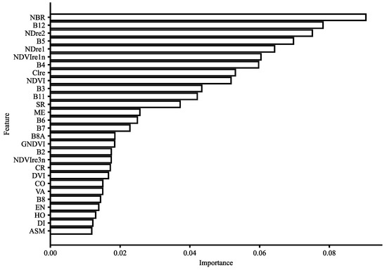
Figure 4.
Predictor variable importance with Gini importance in RF model.
In terms of the SWIR and its relative features, B12 and NBR were the most suitable features for identifying forest logging. The other short-wave infrared band, B11, was not as important but still outperformed some of the conventional bands and most conventional vegetation indices.
In terms of red-edge-related features, NDre1, NDVIre1n, and CIre were also very effective, in addition to B5 and NDre2, which had the greatest ability to identify deforestation. However, B6, B7, B8A, and NDVIre3 were relatively weak and only outperformed the texture features.
The texture features showed relatively low importance in monitoring forest logging patterns. Seven textural features, including CR, CO, and VA, were at the bottom of the list, except for ME, which had a moderate contribution effect.
4. Discussion
Reliable detection of logging patterns is an important component of sustainable forest management, as it allows the accurate mapping of forest loss and guides post-disturbance rehabilitation [49,50]. In terms of the data sources used for detection, optical remote sensing is the most cost-effective solution [51,52,53] despite its weaknesses compared to LiDAR and SAR. Our results validate the feasibility of using multispectral high-resolution optical imagery to identify deforestation patterns at the subcompartment scale. Since logging causes changes in forest composition and canopy structure, which in turn affects the feature spectrum, we were able to capture more details of canopy disturbance such as canopy gaps with high resolution combined with more spectral information such as red-edge and short-wave infrared, which can meet the application requirements. This result is consistent with the results of Francini et al. [54,55].
The inclusion of the red-edge and short-wave infrared bands can significantly improve the accuracy of logging detection, particularly the B5 (698~713 nm) and B12 (2100–2280 nm) bands of Sentinel-2. In terms of the red-edge bands, as the B5 band is associated with changes in chlorophyll content [56], vegetation indices associated with the B5 band such as NDre2, NDre1, NDVIre1n, and Cire all perform well, and are suitable for differentiating logging pattern, in agreement with the results of Fernández-Manso et al. [38]. Particularly NDre can detect phenomena such as defoliation caused by disturbance events in the forest earlier than conventional indices [57,58]. In terms of the short-wave infrared band, because B12 is highly correlated with biochemicals such as leaf pigment and moisture and can pass through thin cloud cover, it indicates forest disturbance well [59]. NBR is calculated from B12 and the near-infrared band. Sub-pixel-level canopy disturbance events in the evergreen forests of Southeast Asia can be detected using changes in NBR alone [60]. Short-wave infrared bands are superior to using only red and NIR bands for monitoring forest disturbances [61,62]. Previous studies have shown that texture features respond significantly to variables that cause changes in canopy structure and play a dominant role in selective logging monitoring in tropical forests [51,63], unlike the results of our study. This may be because the Taizi Mountain area is dominated by plantations of Pinus massoniana Lamb. and Cunninghamia lanceolata (Lamb.), which indicates that there is little variation within the forest stand structure. Another potential reason is that the pixel window is too small to fairly identify selectively logging subcompartments.
The original volume of the stand may influence the detecting results. If the original hectare volume is high, the difference in volume between selective logging and unlogged can hardly be reflected in the spectrum. However, due to the saturation phenomenon in optical remote sensing vegetation analysis [64], it is hard to detect the selective logging pattern in high-volume areas. Because of the low intensity of selective logging and the scattered area of operations, post-logging forest stock may still be above the saturation level of volume estimates. As shown in Figure 5, despite the difference in hectare volume before logging, no significant difference is visible in the RGB images after selective logging. The use of more spectral bands and vegetation indices could improve the saturation values to some extent [65]. Short-wave infrared and red-edge information were shown to reduce this effect and improve the assessment of growing stem volume, but volume estimates are still limited by saturation effects [66,67]. We found that misclassification between selective logging and unlogged was highly likely to occur if the preharvest volume of the subcompartment was above 160 m3/ha. Improvements in feature variable screening methods, innovative algorithms, and fusion of imagery may improve the ability of optical imagery to detect selective logging [68,69].
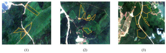
Figure 5.
Selective logging samples with different pre-logging hectare volume. (1) Low pre-logging hectare volume, 48.83~74.19 m3/ha; (2) Medium pre-logging hectare volume, 93.58~146.41 m3/ha; (3) High pre-logging hectare volume, 160~206.89 m3/ha.
In addition, the time lag of the optical image is also an important reason for the misclassification of low-intensity selective felling [70]. Figure 6 illustrates the recovery of coniferous and broadleaved forests over time after clear-cutting. The growing season is characterized by favorable temperatures and abundant rainfall. On the one hand, it makes secondary vegetation regenerate rapidly, resulting in weak and short spectral changes due to logging, and on the other hand, it makes cloud cover long, limiting the optical sensors. Therefore, if the lag time can be reduced, it will effectively improve the observation availability and enhance the performance of systems based on satellite imagery for monitoring forest logging [71]. The integration of multiple sensors is one way to improve temporal accuracy. The integration of optical sensors, such as the combination of Landsat and Sentinel-2 [72], and the integration of optical and radar datasets, such as the combination of Sentinel-1, PALSAR-2, and Landsat datasets [73], will increase the number of available observations and detect forest disturbances earlier [74,75]. Furthermore, the launch of additional satellites will also provide more detailed information for detecting and acting on logging events.
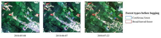
Figure 6.
Change in coniferous and broadleaved forests over time after clear-cutting.
5. Conclusions
This study was conducted to evaluate the combination of visible, near-infrared, red-edge, and short-wave infrared spectral bands derived from Sentinel-2 for identifying three logging patterns (unlogged, selective logging, and clear-cutting) in north subtropical plantation forests. Overall, we found that the optical images have the potential ability to detect logging patterns especially for the clear-cutting and unlogged patterns, which can be well-classified. In addition, the detection accuracy of the selective logging pattern can be improved by adding more spectral bands, especially when adding a red-edge band or short-wave infrared band or both, improving the accuracy by 4–5% in general. Furthermore, the satellite’s ability to monitor the selective logging pattern with the random forest algorithm has been effectively enhanced by adding red-edge and short-wave infrared bands to the traditional visible and near-infrared bands, which can improve precision and recall accuracy by 3–6%, respectively. The red-edge band (698–713 nm, B5 in Sentinel-2), the short-wave infrared (2100–2280 nm, B12 in Sentinel-2) and the associated vegetation indices (NBR, NDre2, and NDre1) showed great potential in detecting logging patterns, and the greatest enhancement was performed on the selective logging pattern.
Author Contributions
Conceptualization, Y.D.; data curation, Y.H., Z.W. and Y.Z.; formal analysis, Y.H. and Y.D.; funding acquisition, Y.D.; methodology, Z.W.; supervision, Y.D.; writing the original draft, Y.H. and Y.D.; Writing—Review and editing, Y.D. All authors have read and agreed to the published version of the manuscript.
Funding
This research was funded by the National Natural Science Foundation of China (Grant No.32071683).
Acknowledgments
In this section, you can acknowledge any support given which is not covered by the author contribution or funding sections. This may include administrative and technical support, or donations in kind (e.g., materials used for experiments).
Conflicts of Interest
The authors declare no conflict of interest.
References
- Wu, S.; Yan, X.; Zhang, L. The relationship between forest ecosystem emergy and forest ecosystem service value in China. Acta Geogr. Sin. 2014, 69, 334–342. [Google Scholar] [CrossRef]
- Zou, W.; Chen, S.; Zhao, R. Research Advances in Remote Sensing Based Monitoring of Carbon Storage and Carbon Fluxes in Forest Ecosystem. World For. Res. 2017, 30, 1–7. [Google Scholar] [CrossRef]
- Lambert, J.; Denux, J.-P.; Verbesselt, J.; Balent, G.; Cheret, V. Detecting Clear-Cuts and Decreases in Forest Vitality Using MODIS NDVI Time Series. Remote Sens. 2015, 7, 3588–3612. [Google Scholar] [CrossRef]
- Borrelli, P.; Modugno, S.; Panagos, P.; Marchetti, M.; Schütt, B.; Montanarella, L. Detection of harvested forest areas in Italy using Landsat imagery. Appl. Geogr. 2014, 48, 102–111. [Google Scholar] [CrossRef]
- Pi, X.; Zeng, Y.; He, C. Estimating urban vegetation coverage on the basis of multi-source remote sensing data and temporal mixture analysis. Natl. Remote Sens. Bull. 2021, 25, 1216–1226. [Google Scholar] [CrossRef]
- Wang, M.; Zhang, X.; Wang, J.; Sun, Y.; Jian, G.; Pan, C. Forest resource classification based on random forest and object oriented method. Acta Geod. Et Cartogr. Sin. 2020, 49, 235–244. [Google Scholar] [CrossRef]
- Zarco-Tejada, P.J.; Hornero, A.; Hernández-Clemente, R.; Beck, P.S.A. Understanding the temporal dimension of the red-edge spectral region for forest decline detection using high-resolution hyperspectral and Sentinel-2a imagery. ISPRS J. Photogramm. Remote Sens. 2018, 137, 134–148. [Google Scholar] [CrossRef]
- Rao, Y.; Wang, C.; Huang, H. Forest fire monitoring based on multisensor remote sensing techniques in Muli County, Sichuan Province. Natl. Remote Sens. Bull. 2020, 24, 559–570. [Google Scholar] [CrossRef]
- Yu, W.; Zhao, P.; Xu, K.; Zhao, Y.; Shen, P.; Ma, J. Evaluation of red-edge features for identifying subtropical tree species based on Sentinel-2 and Gaofen-6 time series. Int. J. Remote Sens. 2022, 43, 3003–3027. [Google Scholar] [CrossRef]
- Liu, Q.; Qin, X.; Hu, X.; Li, Z. Spectral and Index Analysis for Burned Areas Identification Using GF-6 WFV Data. Spectrosc. Spectr. Anal. 2021, 41, 2536–2542. [Google Scholar] [CrossRef]
- Huang, J.; Li, Z.; Chen, E.; Zhao, L.; Mo, B. Classification of plantation types based on WFV multispectral imagery of the GF-6 satellite. Natl. Remote Sens. Bull. 2021, 25, 539–548. [Google Scholar] [CrossRef]
- Parida, B.R.; Kumari, A. Mapping and modeling mangrove biophysical and biochemical parameters using Sentinel-2A satellite data in Bhitarkanika National Park, Odisha. Model. Earth Syst. Environ. 2021, 7, 2463–2474. [Google Scholar] [CrossRef]
- Darvishzadeh, R.; Skidmore, A.; Abdullah, H.; Cherenet, E.; Ali, A.; Wang, T.; Nieuwenhuis, W.; Heurich, M.; Vrieling, A.; O’Connor, B.; et al. Mapping leaf chlorophyll content from Sentinel-2 and RapidEye data in spruce stands using the invertible forest reflectance model. Int. J. Appl. Earth Obs. Geoinf. 2019, 79, 58–70. [Google Scholar] [CrossRef]
- Souza, C.M.; Roberts, D. Mapping forest degradation in the Amazon region with Ikonos images. Int. J. Remote Sens. 2005, 26, 425–429. [Google Scholar] [CrossRef]
- Souza, J.C.; Siqueira, J.; Sales, M.; Fonseca, A.; Ribeiro, J.; Numata, I.; Cochrane, M.; Barber, C.; Roberts, D.; Barlow, J. Ten-Year Landsat Classification of Deforestation and Forest Degradation in the Brazilian Amazon. Remote Sens. 2013, 5, 5493–5513. [Google Scholar] [CrossRef]
- Bullock, E.L.; Woodcock, C.E.; Olofsson, P. Monitoring tropical forest degradation using spectral unmixing and Landsat time series analysis. Remote Sens. Environ. 2020, 238, 110968. [Google Scholar] [CrossRef]
- Grecchi, R.C.; Beuchle, R.; Shimabukuro, Y.E.; Aragão, L.E.O.C.; Arai, E.; Simonetti, D.; Achard, F. An integrated remote sensing and GIS approach for monitoring areas affected by selective logging: A case study in northern Mato Grosso, Brazilian Amazon. Int. J. Appl. Earth Obs. Geoinf. 2017, 61, 70–80. [Google Scholar] [CrossRef] [PubMed]
- Johnson, K.M.; Ouimet, W.B.; Dow, S.; Haverfield, C. Estimating Historically Cleared and Forested Land in Massachusetts, USA, Using Airborne LiDAR and Archival Records. Remote Sens. 2021, 13, 4318. [Google Scholar] [CrossRef]
- Antropov, O.; Rauste, Y.; Praks, J.; Seifert, F.M.; Häme, T. Mapping Forest Disturbance Due to Selective Logging in the Congo Basin with RADARSAT-2 Time Series. Remote Sens. 2021, 13, 740. [Google Scholar] [CrossRef]
- Ota, T.; Ahmed, O.S.; Minn, S.T.; Khai, T.C.; Mizoue, N.; Yoshida, S. Estimating selective logging impacts on aboveground biomass in tropical forests using digital aerial photography obtained before and after a logging event from an unmanned aerial vehicle. For. Ecol. Manag. 2019, 433, 162–169. [Google Scholar] [CrossRef]
- d’Oliveira, M.V.N.; Figueiredo, E.O.; de Almeida, D.R.A.; Oliveira, L.C.; Silva, C.A.; Nelson, B.W.; Da Cunha, R.M.; de Almeida Papa, D.; Stark, S.C.; Valbuena, R. Impacts of selective logging on Amazon forest canopy structure and biomass with a LiDAR and photogrammetric survey sequence. For. Ecol. Manag. 2021, 500, 119648. [Google Scholar] [CrossRef]
- Huertas, C.; Sabatier, D.; Derroire, G.; Ferry, B.; Jackson, T.; Pélissier, R.; Vincent, G. Mapping tree mortality rate in a tropical moist forest using multi-temporal LiDAR. Int. J. Appl. Earth Obs. Geoinf. 2022, 109, 102780. [Google Scholar] [CrossRef]
- Kuck, T.N.; Silva Filho, P.F.F.; Sano, E.E.; Da Bispo, P.C.; Shiguemori, E.H.; Dalagnol, R. Change Detection of Selective Logging in the Brazilian Amazon Using X-Band SAR Data and Pre-Trained Convolutional Neural Networks. Remote Sens. 2021, 13, 4944. [Google Scholar] [CrossRef]
- Zhao, F.; Sun, R.; Zhong, L.; Meng, R.; Huang, C.; Zeng, X.; Wang, M.; Li, Y.; Wang, Z. Monthly mapping of forest harvesting using dense time series Sentinel-1 SAR imagery and deep learning. Remote Sens. Environ. 2022, 269, 112822. [Google Scholar] [CrossRef]
- Jayathunga, S.; Owari, T.; Tsuyuki, S. Digital Aerial Photogrammetry for Uneven-Aged Forest Management: Assessing the Potential to Reconstruct Canopy Structure and Estimate Living Biomass. Remote Sens. 2019, 11, 338. [Google Scholar] [CrossRef]
- Coops, N.C.; Shang, C.; Wulder, M.A.; White, J.C.; Hermosilla, T. Change in forest condition: Characterizing non-stand replacing disturbances using time series satellite imagery. For. Ecol. Manag. 2020, 474, 118370. [Google Scholar] [CrossRef]
- White, J.C.; Hermosilla, T.; Wulder, M.A.; Coops, N.C. Mapping, validating, and interpreting spatio-temporal trends in post-disturbance forest recovery. Remote Sens. Environ. 2022, 271, 112904. [Google Scholar] [CrossRef]
- Cardille, J.A.; Perez, E.; Crowley, M.A.; Wulder, M.A.; White, J.C.; Hermosilla, T. Multi-sensor change detection for within-year capture and labelling of forest disturbance. Remote Sens. Environ. 2022, 268, 112741. [Google Scholar] [CrossRef]
- Drusch, M.; Del Bello, U.; Carlier, S.; Colin, O.; Fernandez, V.; Gascon, F.; Hoersch, B.; Isola, C.; Laberinti, P.; Martimort, P.; et al. Sentinel-2: ESA’s Optical High-Resolution Mission for GMES Operational Services. Remote Sens. Environ. 2012, 120, 25–36. [Google Scholar] [CrossRef]
- Lima, T.A.; Beuchle, R.; Langner, A.; Grecchi, R.C.; Griess, V.C.; Achard, F. Comparing Sentinel-2 MSI and Landsat 8 OLI Imagery for Monitoring Selective Logging in the Brazilian Amazon. Remote Sens. 2019, 11, 961. [Google Scholar] [CrossRef]
- Zheng, D. Analysis of the “Three Total” Inspection Based on Remote Sensing Technology. For. Resour. Manag. 2013, 03, 28–30. [Google Scholar] [CrossRef]
- Brauchler, M.; Stoffels, J.; Nink, S. Extension of an Open GEOBIA Framework for Spatially Explicit Forest Stratification with Sentinel-2. Remote Sens. 2022, 14, 727. [Google Scholar] [CrossRef]
- Verbesselt, J.; Hyndman, R.; Zeileis, A.; Culvenor, D. Phenological change detection while accounting for abrupt and gradual trends in satellite image time series. Remote Sens. Environ. 2010, 114, 2970–2980. [Google Scholar] [CrossRef]
- Shimizu, K.; Ahmed, O.S.; Ponce-Hernandez, R.; Ota, T.; Win, Z.C.; Mizoue, N.; Yoshida, S. Attribution of Disturbance Agents to Forest Change Using a Landsat Time Series in Tropical Seasonal Forests in the Bago Mountains, Myanmar. Forests 2017, 8, 218. [Google Scholar] [CrossRef]
- Meyer, L.H.; Heurich, M.; Beudert, B.; Premier, J.; Pflugmacher, D. Comparison of Landsat-8 and Sentinel-2 Data for Estimation of Leaf Area Index in Temperate Forests. Remote Sens. 2019, 11, 1160. [Google Scholar] [CrossRef]
- Chaves, M.E.D.; Picoli, M.C.A.; Sanches, I.D. Recent Applications of Landsat 8/OLI and Sentinel-2/MSI for Land Use and Land Cover Mapping: A Systematic Review. Remote Sens. 2020, 12, 3062. [Google Scholar] [CrossRef]
- Dong, T.; Liu, J.; Shang, J.; Qian, B.; Ma, B.; Kovacs, J.M.; Walters, D.; Jiao, X.; Geng, X.; Shi, Y. Assessment of red-edge vegetation indices for crop leaf area index estimation. Remote Sens. Environ. 2019, 222, 133–143. [Google Scholar] [CrossRef]
- Navarro, G.; Caballero, I.; Silva, G.; Parra, P.-C.; Vázquez, Á.; Caldeira, R. Evaluation of forest fire on Madeira Island using Sentinel-2A MSI imagery. Int. J. Appl. Earth Obs. Geoinf. 2017, 58, 97–106. [Google Scholar] [CrossRef]
- Wu, Z.; Snyder, G.; Vadnais, C.; Arora, R.; Babcock, M.; Stensaas, G.; Doucette, P.; Newman, T. User needs for future Landsat missions. Remote Sens. Environ. 2019, 231, 111214. [Google Scholar] [CrossRef]
- Fernández-Manso, A.; Fernández-Manso, O.; Quintano, C. SENTINEL-2A red-edge spectral indices suitability for discriminating burn severity. Int. J. Appl. Earth Obs. Geoinf. 2016, 50, 170–175. [Google Scholar] [CrossRef]
- Hall-Beyer, M. Practical guidelines for choosing GLCM textures to use in landscape classification tasks over a range of moderate spatial scales. Int. J. Remote Sens. 2017, 38, 1312–1338. [Google Scholar] [CrossRef]
- Jian, Y.; Han, Z.; Huang, G.; Wang, X.; Li, Y.; Zhou, J.; Dian, Y. Estimation of forest biomass using high spatial resolution remote sensing imagery in north subtropical forests. Acta Ecologica Sinica 2021, 41, 2161–2169. [Google Scholar] [CrossRef]
- Hethcoat, M.G.; Edwards, D.P.; Carreiras, J.M.B.; Bryant, R.G.; França, F.M.; Quegan, S. A machine learning approach to map tropical selective logging. Remote Sens. Environ. 2019, 221, 569–582. [Google Scholar] [CrossRef]
- Haralick, R.M.; Shanmugam, K.; Dinstein, I. Textural features for image classification. IEEE Trans. Syst. Man Cyber. 1973, SMC-3, 610–621. [Google Scholar] [CrossRef]
- Ye, T.; Wang, Y.; Guo, Z.; Li, Y. Factor contribution to fire occurrence, size, and burn probability in a subtropical coniferous forest in East China. PLoS ONE 2017, 12, e0172110. [Google Scholar] [CrossRef]
- Breiman, L. Random Forests. Mach. Learn. 2001, 45, 5–32. [Google Scholar] [CrossRef]
- Gordon, A.D.; Breiman, L.; Friedman, J.H.; Olshen, R.A.; Stone, C.J. Classification and Regression Trees. Biometrics 1984, 40, 874. [Google Scholar] [CrossRef]
- Yue, J.; Yang, G.; Feng, H. Comparative of remote sensing estimation models of winter wheat biomass based on random forest algorithm. Trans. Chin. Soc. Agric. Eng. 2016, 32, 175–182. [Google Scholar] [CrossRef]
- Hari Poudyal, B.; Maraseni, T.; Cockfield, G. Evolutionary dynamics of selective logging in the tropics: A systematic review of impact studies and their effectiveness in sustainable forest management. For. Ecol. Manag. 2018, 430, 166–175. [Google Scholar] [CrossRef]
- Hirschmugl, M.; Gallaun, H.; Dees, M.; Datta, P.; Deutscher, J.; Koutsias, N.; Schardt, M. Methods for Mapping Forest Disturbance and Degradation from Optical Earth Observation Data: A Review. Curr. Forestry Rep. 2017, 3, 32–45. [Google Scholar] [CrossRef]
- Abdollahnejad, A.; Panagiotidis, D.; Bílek, L. An Integrated GIS and Remote Sensing Approach for Monitoring Harvested Areas from Very High-Resolution, Low-Cost Satellite Images. Remote Sens. 2019, 11, 2539. [Google Scholar] [CrossRef]
- Hemmerling, J.; Pflugmacher, D.; Hostert, P. Mapping temperate forest tree species using dense Sentinel-2 time series. Remote Sens. Environ. 2021, 267, 112743. [Google Scholar] [CrossRef]
- Szostak, M.; Hawryło, P.; Piela, D. Using of Sentinel-2 images for automation of the forest succession detection. Eur. J. Remote Sens. 2018, 51, 142–149. [Google Scholar] [CrossRef]
- Francini, S.; McRoberts, R.E.; D’Amico, G.; Coops, N.C.; Hermosilla, T.; White, J.C.; Wulder, M.A.; Marchetti, M.; Mugnozza, G.S.; Chirici, G. An open science and open data approach for the statistically robust estimation of forest disturbance areas. Int. J. Appl. Earth Obs. Geoinf. 2022, 106, 102663. [Google Scholar] [CrossRef]
- St Peter, J.; Anderson, C.; Drake, J.; Medley, P. Spatially Quantifying Forest Loss at Landscape-scale Following a Major Storm Event. Remote Sens. 2020, 12, 1138. [Google Scholar] [CrossRef]
- Sun, L.; Chen, J.; Guo, S.; Deng, X.; Han, Y. Integration of Time Series Sentinel-1 and Sentinel-2 Imagery for Crop Type Mapping over Oasis Agricultural Areas. Remote Sens. 2020, 12, 158. [Google Scholar] [CrossRef]
- Marx, A.; Kleinschmit, B. Sensitivity analysis of RapidEye spectral bands and derived vegetation indices for insect defoliation detection in pure Scots pine stands. iForest 2017, 10, 659–668. [Google Scholar] [CrossRef]
- Bałazy, R.; Hycza, T.; Kamińska, A.; Osińska-Skotak, K. Factors Affecting the Health Condition of Spruce Forests in Central European Mountains-Study Based on MultitemporalRapidEye Satellite Images. Forests 2019, 10, 943. [Google Scholar] [CrossRef]
- Peña, M.A.; Liao, R.; Brenning, A. Using spectrotemporal indices to improve the fruit-tree crop classification accuracy. ISPRS J. Photogramm. Remote Sens. 2017, 128, 158–169. [Google Scholar] [CrossRef]
- Langner, A.; Miettinen, J.; Kukkonen, M.; Vancutsem, C.; Simonetti, D.; Vieilledent, G.; Verhegghen, A.; Gallego, J.; Stibig, H.-J. Towards Operational Monitoring of Forest Canopy Disturbance in Evergreen Rain Forests: A Test Case in Continental Southeast Asia. Remote Sens. 2018, 10, 544. [Google Scholar] [CrossRef]
- Bullock, E.L.; Woodcock, C.E.; Holden, C.E. Improved change monitoring using an ensemble of time series algorithms. Remote Sens. Environ. 2020, 238, 111165. [Google Scholar] [CrossRef]
- Tang, X.; Bullock, E.L.; Olofsson, P.; Woodcock, C.E. Can VIIRS continue the legacy of MODIS for near real-time monitoring of tropical forest disturbance? Remote Sens. Environ. 2020, 249, 112024. [Google Scholar] [CrossRef]
- Hethcoat, M.G.; Carreiras, J.M.; Edwards, D.P.; Bryant, R.G.; Quegan, S. Detecting tropical selective logging with C-band SAR data may require a time series approach. Remote Sens. Environ. 2021, 259, 112411. [Google Scholar] [CrossRef]
- Holloway-Brown, J.; Helmstedt, K.J.; Mengersen, K.L. Interpolating missing land cover data using stochastic spatial random forests for improved change detection. Remote Sens. Ecol. Conserv. 2021, 7, 649–665. [Google Scholar] [CrossRef]
- Saatchi, S.S.; Houghton, R.A.; Dos Santos Alvalá, R.C.; Soares, J.V.; Yu, Y. Distribution of aboveground live biomass in the Amazon basin. Glob. Change Biol. 2007, 13, 816–837. [Google Scholar] [CrossRef]
- Francini, S.; McRoberts, R.E.; Giannetti, F.; Mencucci, M.; Marchetti, M.; Scarascia Mugnozza, G.; Chirici, G. Near-real time forest change detection using PlanetScope imagery. Eur. J. Remote Sens. 2020, 53, 233–244. [Google Scholar] [CrossRef]
- Chrysafis, I.; Mallinis, G.; Tsakiri, M.; Patias, P. Evaluation of single-date and multi-seasonal spatial and spectral information of Sentinel-2 imagery to assess growing stock volume of a Mediterranean forest. Int. J. Appl. Earth Obs. Geoinf. 2019, 77, 1–14. [Google Scholar] [CrossRef]
- Hu, Y.; Xu, X.; Wu, F.; Sun, Z.; Xia, H.; Meng, Q.; Huang, W.; Zhou, H.; Gao, J.; Li, W.; et al. Estimating Forest Stock Volume in Hunan Province, China, by Integrating In Situ Plot Data, Sentinel-2 Images, and Linear and Machine Learning Regression Models. Remote Sens. 2020, 12, 186. [Google Scholar] [CrossRef]
- Li, X.; Liu, Z.; Lin, H.; Wang, G.; Sun, H.; Long, J.; Zhang, M. Estimating the Growing Stem Volume of Chinese Pine and Larch Plantations based on Fused Optical Data Using an Improved Variable Screening Method and Stacking Algorithm. Remote Sens. 2020, 12, 871. [Google Scholar] [CrossRef]
- Melendy, L.; Hagen, S.C.; Sullivan, F.B.; Pearson, T.; Walker, S.M.; Ellis, P.; Kustiyo; Sambodo, A.K.; Roswintiarti, O.; Hanson, M.A.; et al. Automated method for measuring the extent of selective logging damage with airborne LiDAR data. ISPRS J. Photogramm. Remote Sens. 2018, 139, 228–240. [Google Scholar] [CrossRef]
- Hansen, M.C.; Krylov, A.; Tyukavina, A.; Potapov, P.V.; Turubanova, S.; Zutta, B.; Ifo, S.; Margono, B.; Stolle, F.; Moore, R. Humid tropical forest disturbance alerts using Landsat data. Environ. Res. Lett. 2016, 11, 34008. [Google Scholar] [CrossRef]
- Chen, N.; Tsendbazar, N.-E.; Hamunyela, E.; Verbesselt, J.; Herold, M. Sub-annual tropical forest disturbance monitoring using harmonized Landsat and Sentinel-2 data. Int. J. Appl. Earth Obs. Geoinf. 2021, 102, 102386. [Google Scholar] [CrossRef]
- Reiche, J.; Hamunyela, E.; Verbesselt, J.; Hoekman, D.; Herold, M. Improving near-real time deforestation monitoring in tropical dry forests by combining dense Sentinel-1 time series with Landsat and ALOS-2 PALSAR-2. Remote Sens. Environ. 2018, 204, 147–161. [Google Scholar] [CrossRef]
- Joshi, N.; Baumann, M.; Ehammer, A.; Fensholt, R.; Grogan, K.; Hostert, P.; Jepsen, M.; Kuemmerle, T.; Meyfroidt, P.; Mitchard, E.; et al. A Review of the Application of Optical and Radar Remote Sensing Data Fusion to Land Use Mapping and Monitoring. Remote Sens. 2016, 8, 70. [Google Scholar] [CrossRef]
- Higginbottom, T.P.; Symeonakis, E.; Meyer, H.; van der Linden, S. Mapping fractional woody cover in semi-arid savannahs using multi-seasonal composites from Landsat data. ISPRS J. Photogramm. Remote Sens. 2018, 139, 88–102. [Google Scholar] [CrossRef]
Publisher’s Note: MDPI stays neutral with regard to jurisdictional claims in published maps and institutional affiliations. |
© 2022 by the authors. Licensee MDPI, Basel, Switzerland. This article is an open access article distributed under the terms and conditions of the Creative Commons Attribution (CC BY) license (https://creativecommons.org/licenses/by/4.0/).