Optimizing Management Practices to Reduce Sediment Connectivity between Forest Roads and Streams in a Mountainous Watershed

Abstract

Forest roads often increase runoff and sediment loss, thus greatly impacting hydrological processes in mountainous watersheds. While there has been previous investigation on best management practices (BMPs) to reduce soil erosion from forest roads, few studies have attempted to optimize BMPs based on how much they can decrease sediment connectivity between forest roads and streams. To close this gap in knowledge, we analyzed the spatial relationship between forest roads and streams, presented the spatial distribution of sediment connectivity by integrating the forest roads into the calculation of the index of connectivity (IC), determined how sediment connectivity would respond to additional BMPs through simulating scenarios, and used these data to optimize the BMPs so they would intercept the greatest sediment loads. We found that forest roads and streams in the Xiangchagou watershed in the Dabie Mountain area of China tend to occur within 180 m of each other; however, within the same buffer zones, streams are more often accompanied by forest roads. IC was greatest near road–stream crossings but smaller near streams and forest roads, and it tended to decrease as the buffer distance increased. Furthermore, we found that sediment connectivity was decreased through running a variety of scenarios that used sediment basin and riparian buffers as BMPs between forest roads and streams. Specifically, within this watershed, riparian buffers should be 64 m wide, and there should be 30 sediment basins with a minimum upslope drainage area of 2 ha. At these quantities, the BMPs in this watershed would significantly affect sediment connectivity. By contrast, beyond these thresholds, increasing the width of riparian buffers or the number of sediment basins does not lead to meaningful sediment reductions. In this way, we were able to use the mean change point method to determine the optimal sediment basin quantity (30 with corresponding minimum upslope drainage area of 2 ha) and the optimal riparian buffer width (64 m) for the Xiangchagou watershed. While these results are a first approximation in a novel research area, they can guide forest managers and stakeholders to design and optimize BMPs that control the delivery of eroded sediments associated with forest roads.

1. Introduction

While forest roads are vital for facilitating tourism, travel, and timber management and harvesting in mountainous watersheds, they adversely affect these ecosystems’ structures, processes, and function [1,2]. Although forest roads occupy a small percentage of the total area of a watershed, their impervious pavement and general design can cause rainfall to splash and runoff to scour the surface, hitting sediment particles with such intensity that they detach and erode [3,4]. This alters the topographical and hydrological characteristics of the watershed, generating and transporting larger volumes and faster flow of water and sediment [5,6], which follow more complex transport-and-deposit processes than if they had been able to infiltrate the soil [7]. Additionally, because forest roads are designed to transport runoff and sediment on the hillslope, they degrade natural drainage networks [8,9] by concentrating runoff and increasing the sediment connectivity between roads and streams [5]. These characteristics synergize to increase the sediment load entering a watershed [10] and the rate at which these pollutants are transported to streams [4]. In this way, forest roads interrupt the production and transport of eroded sediment [11,12], greatly increasing soil erosion [2,13]. Ultimately, forest roads decrease water quality, increase reservoir siltation, reduce aquatic biomass, and degrade aquatic habitats [4,6,14]. Therefore, there is an urgent need to determine optimal management strategies to control soil erosion caused by forest roads in mountainous watersheds.

Roads alter the “natural” source-to-sink movement of sediment by redirecting sediment-loaded runoff, intercepting surface flow and directing it open bodies of water, rather than allowing it to infiltrate [15,16]. This, in turn, redistributes drainage networks, changing the connectivity and spatial distribution of sediment within the watershed [15,16,17,18]. For example, in the karst region of western Oregon, 57% of the road networks were connected to the local stream networks through roadside ditches and culverts, which increased the drainage network density by 21–50% [19]. Because suspended sediment concentration tends to be 250% greater when it is downstream a road–stream crossing compared with a stream crossing [20], more sediment was received by streams, which significantly increased the sediment connectivity of the watershed [18]. Moreover, roads change the topography of an area, thus changing the direction of surface flow and its direct and diffuse connectivity [17]. This increased hydrological and sediment connectivity, decreased the presence time, and increased the intensity of runoff, which increases the frequency and intensity of floods during rainfall events [21]. Therefore, sediment management in mountainous watersheds should center around reducing sediment production and optimizing water and sediment transport processes from forest roads to streams [22]. While previous best management practices (BMPs) meant to control road erosion were designed to minimize sediment generated by roads, they were less successful at addressing the transportation of runoff and sediment, especially in connections between forest roads and streams.

Sediment connectivity is determined by the topography, soil, vegetation, climate, distance of water flow, and human activity that characterizes the process and potential of sediment to move from a source to a sink in a watershed [11,16]. Therefore, road erosion that influences water and sediment transport processes can be targeted by regulating the sediment connectivity from road to stream [23,24]. For example, Fidelus-Orzechowska et al. [8] demonstrated that BMPs reduce sediment delivery at stream crossings. Sosa-Pérez et al. [16] found that road decommissioning treatments reduced road–stream connectivity. Rachels et al. [25] used sediment source fingerprinting techniques to determine that BMPs were relatively effective at minimizing sediment delivery from roads following forest harvesting. Overall, these recent studies have demonstrated that BMPs can minimize sediment connectivity from forest roads to streams, but this literature is still scarce.

Forest road BMPs tend to utilize engineering and biological measures to regulate road erosion; however, these practices come with ecological and economic trade-offs. Engineering measures tend to direct or interrupt water flow through technologies such as horizontal drainage structures, ditches, sedimentation tanks, silt fences, and reservoirs [26,27]. Biological measures tend to increase surface coverage through biotechnology such as phytoremediation, planting vegetation (grass mat, shrub, etc.), and applying blankets or civil fabric (e.g., shade net, non-woven fabrics, and straw mats) [28,29]. However, installing BMPs to reduce sediment loss can cause other negative environmental impacts, such as increasing deforestation and habitat fragmentation as well as temporarily increasing erosion [2]. Furthermore, these practices can be expensive, which is especially challenging in less economically developed mountainous regions [2,25]. As such, more work is needed to identify specific locations that could most benefit from BMPs and the quantity of BMPs needed for a forested mountainous watershed [30]. For example, BMPs should be installed at a major sediment source or sink to ensure that sediment connectivity between forest roads to streams is reduced [1]. Furthermore, it would provide the most ecological benefit for the money spent on BMPs. In summary, reducing sediment erosion in mountainous watersheds is primarily hindered because there have not been enough BMPs implemented at their greatest source locations.

Although studies have demonstrated that forestry BMPs can reduce sediment erosion, further research is necessary to optimize how BMPs are implemented to improve cost-effectiveness for a given watershed [31]. Despite the clear trade-offs between implementing BMPs and reducing sediment loss in mountainous watersheds, there is no (or little) existing literature comparing these costs and benefits. Therefore, there is a critical need to evaluate the trade-offs from implementing BMPs to determine the optimal balance between effectively controlling sediment losses from forest road to streams and the economic and environmental cost of these practices. Such efforts are needed to help forest managers, stakeholders, and governments allocate resources for watershed management and obtain the greatest benefit.

To meet this need, we used the Xiangchagou watershed in the Dabie Mountain area of China as a case study to guide how the best locations and BMPs can be selected to reduce the most sediment for the lowest cost. The objectives of this study were to (1) clarify spatial relationships between forest roads and streams, (2) analyze how forest roads affect the confluence of water and sediment to change the spatial distribution of sediment connectivity, (3) reveal how different BMPs (sediment basins and riparian buffers) affect the spatial response of sediment connectivity, and (4) determine the specific locations and optimal quantity/width of BMPs to be implemented. By meeting these objectives, we were able to determine which BMP is more successful at reducing sediment connectivity from forest roads to streams as well as recommend the ideal number of sediment basins and the appropriate width of a riparian buffer in a mountainous watershed. When forest roads do not have properly designed and implemented BMPs, they have the potential to drastically alter local hydrology and sediment transportation. However, this study provides BMP recommendations specific to mountainous watersheds to reduce sediment loads entering the watershed.

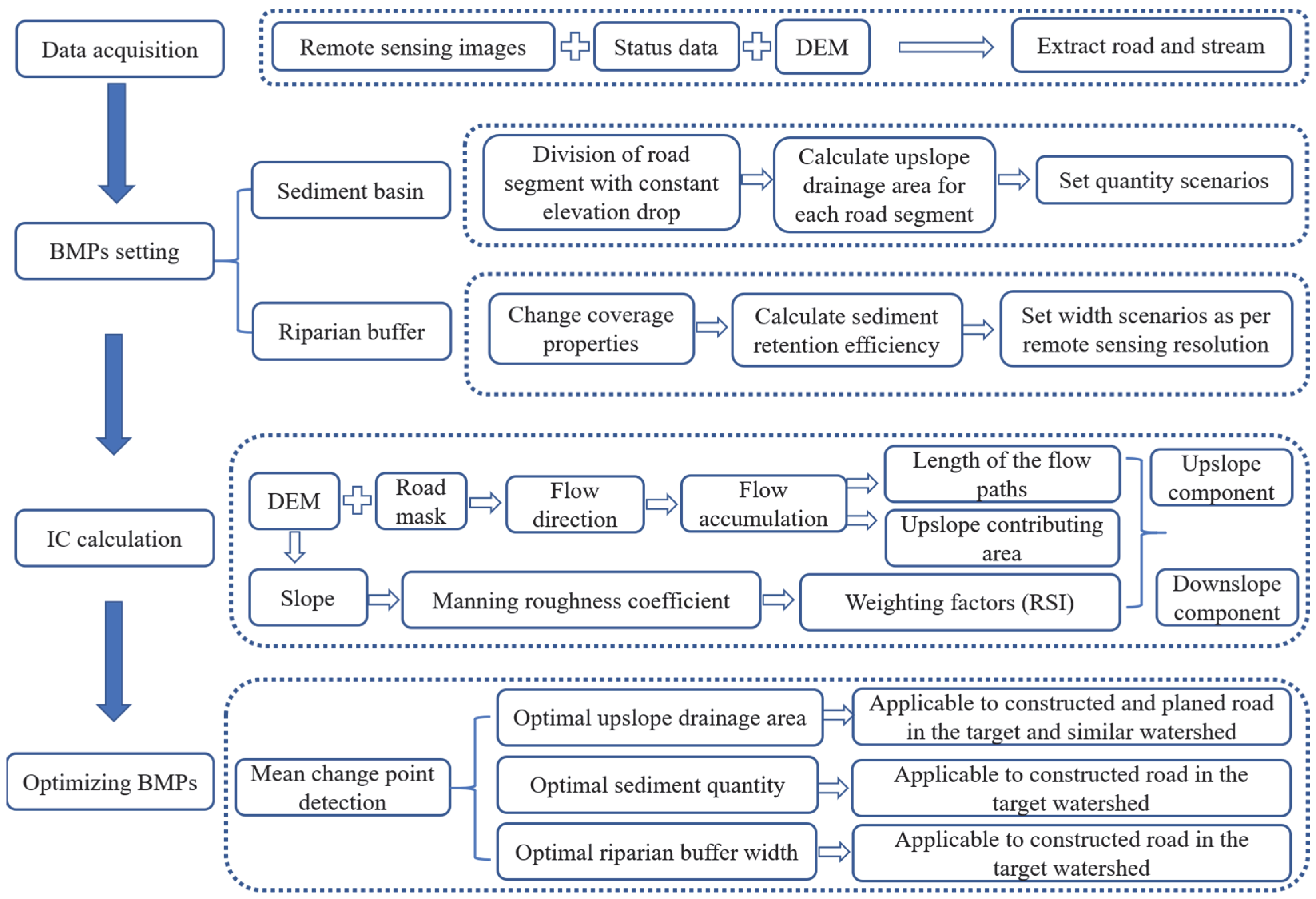
2. Data and Methods

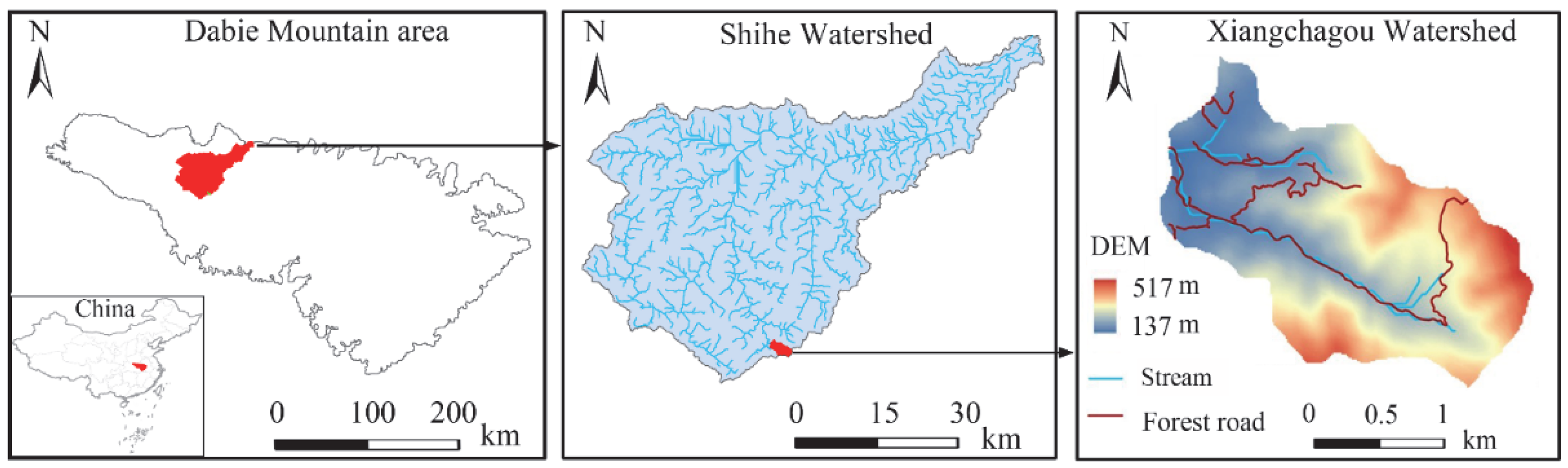
2.1. Study Area

This study was conducted in Xiangchagou (114°1′1″–114°3′30″E, 31°46′5″–31°48′5″N), which is a watershed located on the south facing slopes of the Jigongshan National Nature Reserve, in the province of Henan, central China (Figure 1). The area of this watershed is 6.40 km², and its climate transitions between subtropical and warm temperate with an average annual temperature of 15.2 °C and elevation ranging from 137 to 517 m. Annual rainfall in this region averages 1119 mm, of which more than 80% occurs in the summer, demonstrating high seasonal variability. Xiangchagou’s geology is dominated by mixed granite and composite-granite batholith, and its soils are primarily yellow-brown loams with a depth of 20–50 cm and a pH of 5–6. This region is highly forested, dominated by both deciduous broad-leaved forests and mixed deciduous evergreen and broad-leaved forests. The forests are well-preserved, with more than 90% canopy cover. The dominant tree species include Chinese cork oak (Quercus variabilis Bl.), sawtooth oak (Quercus acutissima Carruth.), mono maple (Acer pictum subsp. mono (Maxim.) H. Ohashi), liquidambar formosana (Liquidambar formosana Hance), and Bunge hackberry (Celtis bungeana Bl.). Forest roads were constructed throughout this region for forest production, harvesting, tourism, and management, and they are 11.26 km in length. Because these roads were poorly designed and maintained, they have been severely eroded and have developed rills and gullies. Thus, they act as a source of and pathway for sediment and runoff [12].

2.2. Data Acquisition

Digital elevation data are the fundamental foundation on the index of connectivity (IC) and its parameters (including flow direction, slope, accumulated drainage area, and flow path). We used August 2018 data from a digital elevation model (DEM) which were composed from the 91 satellite map assistant software (version 5.3.1 with Google Earth v6.0.3; Google, Mountain View, CA, USA) developed by the Beijing Qian Fan Shijing Technology Co., Ltd. (Beijing, China) at a resolution of 16 m. The DEM data were imported into ArcGIS 10.2 (Esri, Redlands, CA, USA), and the hydrological analysis tool was used to identify the topographical characteristics, watershed boundaries, and streams for the Xiangchagou watershed. We visually inspected November 2018 Google Earth images with a resolution of 0.5 m to identify forest roads. Once the streams and forest roads were located, they were calibrated and validated against data provided by the Administrative Bureau of Jigongshan National Nature Reserve as well as the field observations.

2.3. Measurement of Sediment Connectivity

Sediment connectivity is a concept proposed by Ramos-Scharrón et al. [32] in geomorphological studies to determine how efficiently sediment is connected and transmitted between the source (road) and sink (stream) of a watershed, which can aid in identifying “hotspots” that are seriously affected by soil erosion. This information can be used to prioritize BMP placement, thus aiding in the design of comprehensive and effective management strategies [33]. Previous studies have used indicators or approaches to calculate sediment connectivity, such as the sediment delivery ratio (SDR), the volume to breakthrough approach [34], the flow length [35], the graph theory [33], and the sediment flow connectivity index (SCI) [36]. We used the index of connectivity (IC), which was proposed by Borselli et al. [37] to describe the dynamics of sediment transport processes at the watershed scale, specifically the potential of sediment to be transported from source (forest roads) to sink (streams). IC was calculated from the DEM-provided terrain data, in addition to weighting factors, and roads and streams data from ArcGIS 10.2, using the following equations [37]:

$$IC={\log }_{10}\left(\frac{D_{up}}{D_{dn}}\right)$$

(1)

where D_up is the upslope component of IC, and it describes the potential for eroded upslope sediments to flow downstream based on the following equation:

$$D_{up}=\overline{W}\overline{S}\sqrt{A}$$

(2)

where $\overline{W}$ represents the average weighting factor for the upslope contributing area with an average slope of $\overline{S}$ (m/m) and size of A (m²). D_dn is the downslope component of IC, and it describes the potential for sediment produced upslope to move downslope based on the length of the pathways from the source of sediment to the outlet (sink) of the watershed. D_dn is calculated using the following equation:

$$D_{dn}={\displaystyle \sum _i\frac{d_i}{W_i{S}_i}}$$

(3)

where d_i is the length (m) of the flow pathways along the grid cells based on which grid cells are the steepest. W_i and S_i are the weighting factor and slope of the grid cell i, respectively. Note that the weighting factor for IC is usually the C factor for universal soil loss equation (USLE), but we replaced the C factor with the relative smoothness index (RSI) in this study. We made this modification because the C factor insufficiently reflects the surface characteristics of a forested mountainous watershed, even though it considers how resistant a given landscape is to runoff and sediment flux [12,23]. RSI is a dimensionless parameter ranging from 0 to 1, so it preserves the dimensionlessness of the IC weighting factor [38]. It is calculated using the following equation:

$$RSI=\frac{{\displaystyle n_{Min}}}{n}$$

(4)

where RSI is the relative smoothness index. n is the Manning roughness coefficient derived from the following experiential relationship:

$$M=2.4234\times {\displaystyle e^{0.3005\ln \left(n\right)}}$$

(5)

where M is the terrain roughness derived from the DEM based on the following equation:

$$M=1/\cos \alpha$$

(6)

where α is the slope gradient. The calculated RSI value for the Xiangchagou catchment is shown in Figure 2.

Based on these definitions and equations, IC in this region ranges from [–∞, +∞], with larger values indicating higher sediment connectivity [37]. However, these results obscure important factors affecting how forest roads act as drainage pathways and sinks for sediment transport, such as the pathways’ flow direction, number, and length [9]. Therefore, to more accurately represent the impact of forest roads on IC at a mesoscale resolution (16 m), we superimposed a raster map of forest roads onto the initial flow direction as a mask to generate the new flow direction layer, which allowed us to obtain a new flow accumulation layer. This new flow accumulation layer was combined with the stream and road mask layers to quantify D_up and D_dn and calculate the final IC. Our methodology superimposing the road raster layer onto the initial flow direction layer, recalculating the stream mask, and regenerating flow accumulation not only changed the final flow direction but also the potential for sediment produced upslope to move downslope and the length of the flow path required for sediment to reach the nearest sink [9,12].

2.4. Buffer Analysis

Previous studies have indicated that the distance between roads and streams significantly influences the sediment connectivity within a watershed [9,39]. Therefore, analyzing the spatial proximity between roads and streams illuminates road–stream connectivity. We used the “Analysis Tools” in ArcGIS 10.2 to run a buffer analysis to determine the spatial relationships between forest roads and streams and how IC responded to distances between forest roads, streams, and road–stream crossings. We did this by creating a series of seven parallel buffer zones for roads and streams and seven circular buffer zones for road–stream crossings at intervals of 30 m.

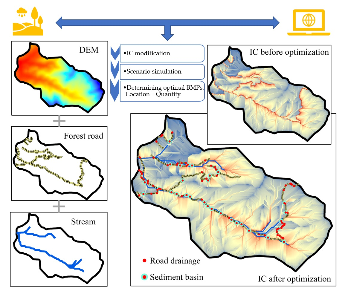
2.5. Optimizing BMPs

Factors that influence sediment transport efficiency and sediment connectivity on road–stream hillslopes include the intensity and duration of rainfall [40], contributing drainage area [11], type of drainage structure employed [40], distance between road and stream [11], downslope terrain and vegetation characteristics [40], and the flow path’s infiltration and sediment storage capacity [11]. Accordingly, BMPs that mitigate or interrupt these factors should be effective in reducing sediment connectivity from forest roads to streams in mountainous watershed [16,24]. As such, we used sediment basins and riparian buffers which are common BMPs and, respectively, representative of engineering and biological measures, as cases to show how BMP placement can be optimized based on IC. The flow diagram of the methodological framework used in this study is shown in Figure 3. For full details of the methods, see the below sections.

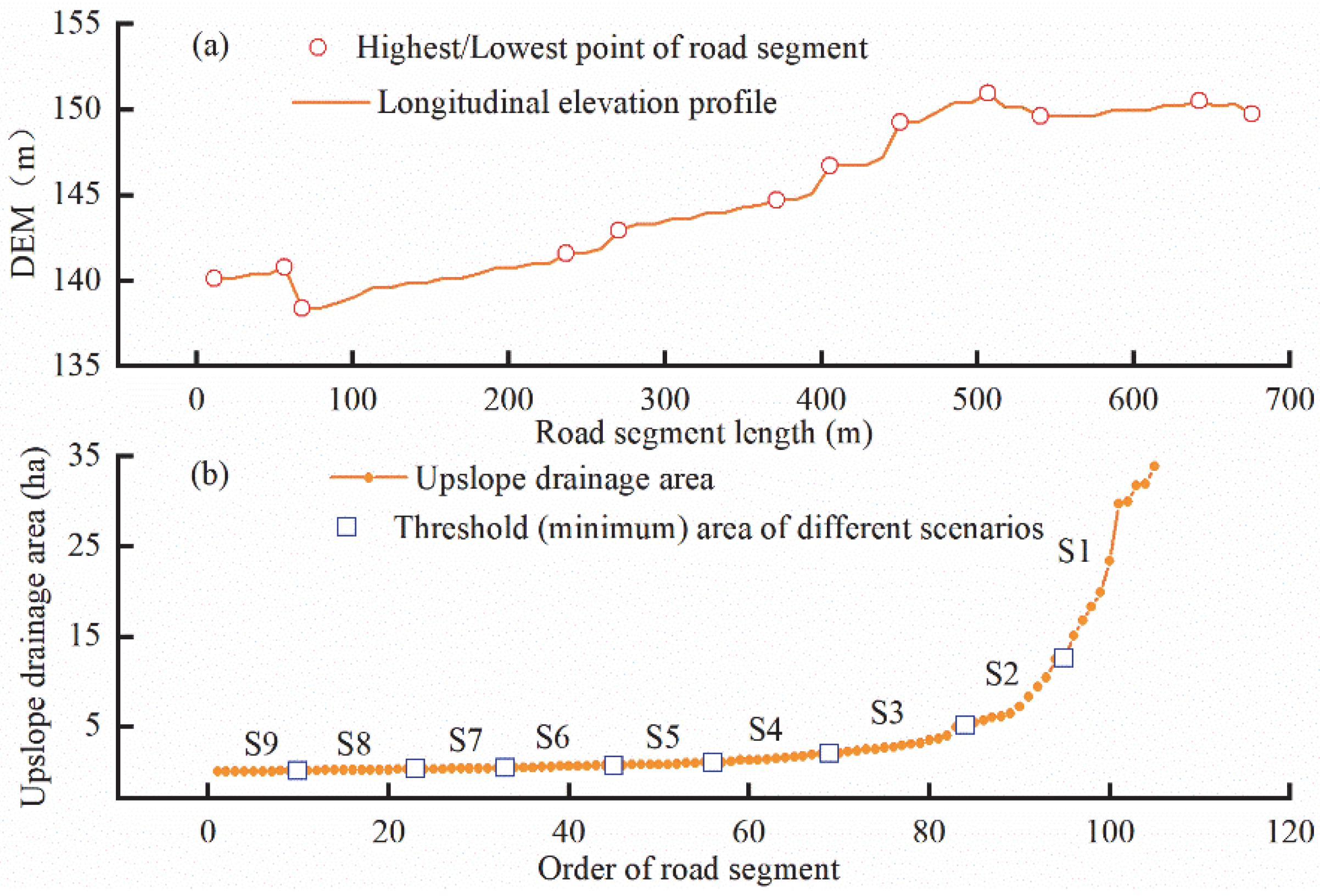
2.5.1. Sediment Basin

Sediment basins can be implemented at road drains to intercept and collect the sediment discharged from the road and uphill slopes, thus reducing sediment connectivity and load. The placement of this “engineering measure” should be informed by the watershed’s topography, how and where roads are distributed, how much the BMP costs, and how much it will disturb the forest ecosystem. With this in mind, sediment basins should be placed such that they intercept the greatest load of sediment with the least sediment basins.

We used the DEM and location of forest roads in the Xiangchagou watershed to portray the longitudinal profiles of the forest roads. We then extrapolated road segments that varied in length but had consistent, 2 m elevation changes (see Figure 4a for an example). Based on these profiles, we selected 105 road segments and assumed that it would be possible to install drainage outlets and sediment basins at the lower elevation of each segment, unless the segments intersected (roads crossings). If segments intersected, we assumed they could share the same outlet for drainage. Accordingly, we determined that 90 road segments could be equipped with drainage outlets and sediment basins, and that this was the maximum number of drainage outlets and sediment basin that can be set along the forest roads in this study area.

Theoretically, installing all 90 sediment basins (Sink_90) would intercept the greatest load of sediment. At the same time, this maximum number would have the greatest construction cost and ecosystem disturbance. To optimize the number of sediment basins, we created eight other scenarios: 80 basins (Sink_80), 70 basins (Sink_70), 60 basins (Sink_60), 50 basins (Sink_50), 40 basins (Sink_40), 30 basins (Sink_30), 20 basins (Sink_20), and 10 basins (Sink_10). Previous studies have established that forest road segments with larger upslope drainage areas contribute more runoff and sediment downslope [3,41]; thus, we determined the best location for sediment basins in these scenarios by identifying which road segments had the largest upslope drainage areas. We calculated the upslope drainage area that would be intercepted by each road segment using the following equation:

$$A=\left(n+1\right)\times D{X}^2$$

(7)

where A represents the upslope drainage area, n represents the number of grid cells occupying the area of the road segment that intercepts runoff and sediment, and DX represents the grid cell size. Once we calculated the upslope drainage area of each road segment, we sorted all road segments accordingly, as shown in Figure 4b. We then assumed that the sediment basin would be at road segments with the greatest upslope drainage area for our eight scenarios.

2.5.2. Riparian Buffer

Riparian buffers can effectively retain sediment, reducing the sediment connectivity between roads and streams [42]; however, their impact correlates strongly with their width [43]. Specifically, while riparian buffers can usually retain more sediment as their buffer width increases, their widths can reach a certain threshold, or turning point, where this relationship is no longer true [43,44]. Accordingly, we created 10 scenarios of riparian buffer with different widths but the same vegetation type to analyze how IC varied in each scenario and to determine the optimal width of riparian buffers in the Xiangchagou watershed. The relationship between the riparian buffer width and sediment retention efficiency was calculated as follows [45]:

$$Y=39.56\times \left(1-\exp \left(-0.035\times x\right)\right);R^2=0.98$$

(8)

where x represents the riparian buffer width and Y represents the sediment retention efficiency. Note that the sediment retention efficiency has an inverse relationship to sediment connectivity. Therefore, the above relationship can be modified as follows to determine a riparian buffer’s width influence on sediment connectivity:

$$y=1-Y$$

(9)

where y represents the sediment transport efficiency at a given riparian buffer width. To reflect how the riparian buffers’ widths affect sediment retention, we run nine scenarios of different riparian buffer widths along the streams at intervals of 16 m (the resolution of DEM data) from streams: at 32 m (buffer_32), 48 m (buffer_48) 64 m (buffer_64), 80 m (buffer_80), 96 m (buffer_96), 112 m (buffer_112), 128 m (buffer_128), 144 m (buffer_144), and 160 m (buffer_160).

In calculating the IC, the weight factor (W_i) represents the force that surface characteristics impose on eroded sediment to block them as they move downslope. This determines how efficiently sediment is transported from upslope to downslope within a watershed, directly impacting the sediment transport process. Because different riparian buffer widths will have varying impacts on sediment connectivity, we assigned a different weight factor to each riparian buffer width so that each IC accurately reflected the varying sediment retention efficiencies (

Table 1. Sediment interception efficiency and sediment transport efficiency of riparian buffers with various widths.

Indicator	Riparian Buffer Width (m)
	16	32	48	64	80	96	112	128	144	160
Sediment retention efficiency Y (%)	0.170	0.267	0.322	0.353	0.372	0.382	0.388	0.391	0.393	0.394
Sediment transport efficiency y (%)	0.830	0.733	0.678	0.647	0.628	0.618	0.612	0.609	0.607	0.606

). This differing weight factor was calculated using the following equation:

$$W=W_i\times y_i$$

(10)

where y_i represents the sediment transport efficiency of the ith riparian buffer width; W_i represents the weight factor used to calculate IC, also known as the relative smoothness index (RSI); and W represents the final weight factor used to calculate IC once the riparian buffer was set.

2.5.3. Mean Change Point Detection

The mean change point is a statistical method used to determine where data experience an abnormal or abrupt change. We used this statistical method to determine the optimal number of sediment basins and the optimal width of riparian buffers. First, we took the logarithm of each scenario’s mean IC value to generate a nonlinear sequence {X_k}, and k = 1, 2, 3, …, and 9. Based on {X_k}, its arithmetic mean value (X) and variance (S) were calculated based on the following equations:

$$X={\displaystyle \sum _{k=1}^n\frac{X_k}{n}}$$

(11)

$$S={\displaystyle \sum _{k=1}^n{(X_k-X)}^2}$$

(12)

where X and S represent the arithmetic mean value and variance, respectively, of the sequence {X_k}. Next, let i = 2, 3, …, and n which divides the sequence {X_k} into two parts {X₁, X₂, …, X_i−1} and {X_i, X_i+1, …, X_n}. Thus, the arithmetic mean value of these two parts and the variance, S_i, were calculated using the following equation:

$$S_i={\displaystyle \sum _{k=1}^{i-1}{(X_k-X_{i1})}^2}+{\displaystyle \sum _{k=i}^n{(X_k-X_{i2})}^2}$$

(13)

where X_i1 and X_i2 represent the arithmetic mean of the sequence {X₁, X₂, …, X_i−1} and {X_i, X_i+1, …, X_n}, respectively. Finally, let IC_i = S − S_i, where the maximum of IC_i corresponds to the optimal number of sediment basins or the optimal width of riparian buffers.

3. Results

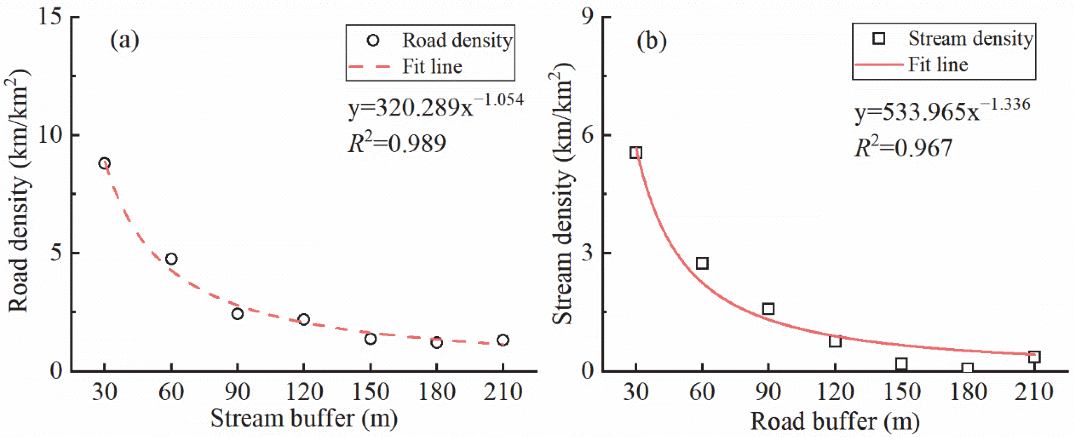
3.1. Spatial Relationship between Roads and Streams

Forest roads and streams tend to exist close to each other, and their proximity determines how easily eroded sediments will move between roads and streams (“road–stream connectivity”) within a watershed. In this study, we used a buffer analysis to detect the variation in stream density along forest roads and road density along streams. Within the Xiangchagou watershed, road densities (km/km²) along streams ranged from a maximum of 8.80 within a 30 m buffer zone to a minimum of 1.21 within a 180 m buffer zone (Figure 5a). By contrast, the stream densities (km/km²) along forest roads ranged from a maximum of 5.55 within a 30 m buffer zone to a minimum of 0.06 within a 180 m buffer zone (Figure 5b). While the density of forest roads and streams decreased as buffer zones increased, the rate of this decline also decreased. Frequency distributions representing the buffer zone distances between forest roads and streams indicate that most are within 180 m of each other. However, within a given buffer zone distance, forest road densities along streams are greater than stream densities along forest roads. This indicates that in the Xiangchagou watershed, streams are often accompanied by forest roads, but forest roads are less likely to be built along streams.

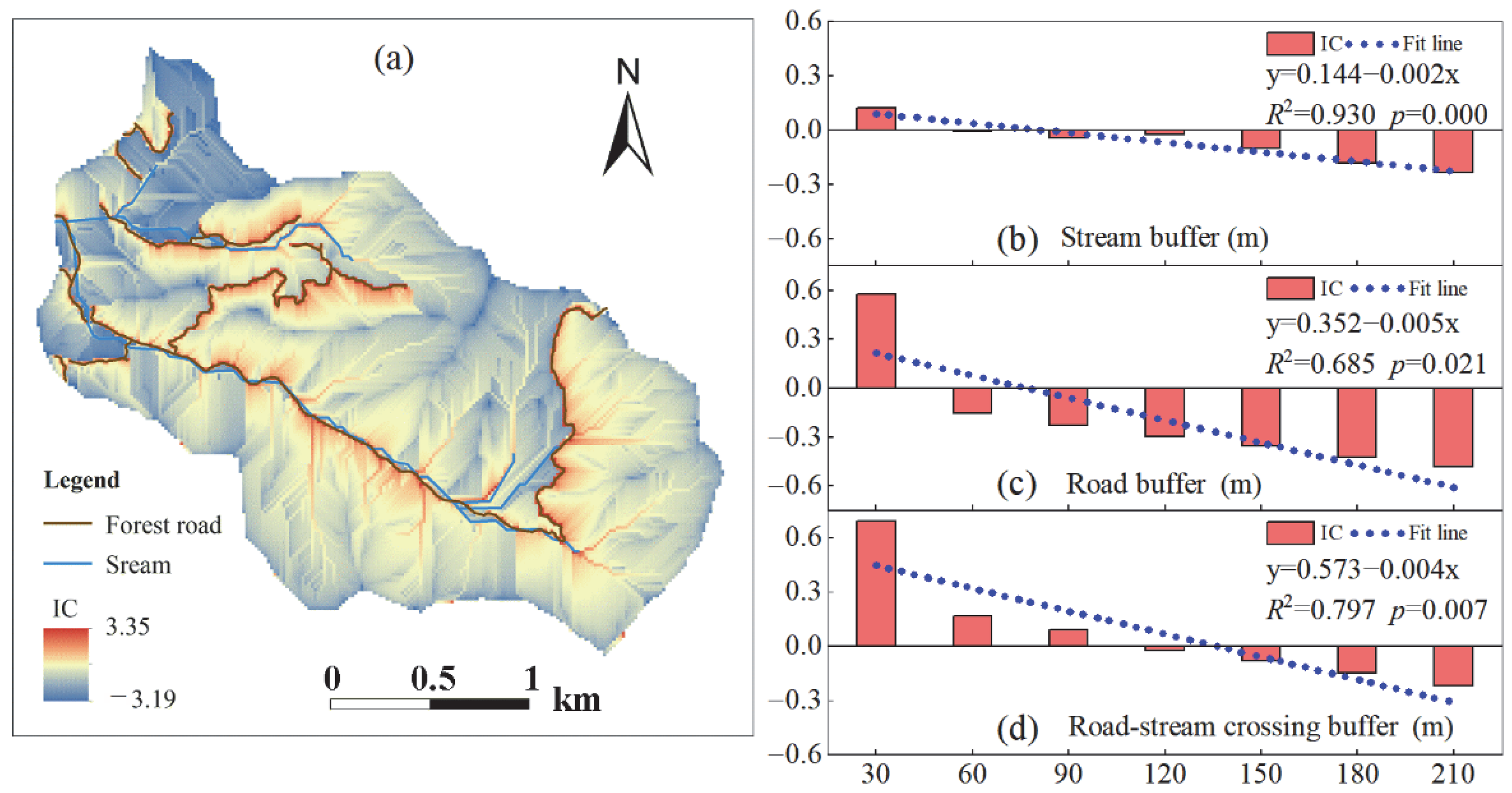
3.2. Spatial Distribution of Sediment Connectivity

The map of sediment connectivity, as calculated by IC, is shown in Figure 6a. Within the Xiangchagou watershed, IC values ranged from −3.19 to 3.35. IC, and thus, sediment connectivity was generally higher near the streams and forest roads, especially in the upper hillslopes of forest roads. By contrast, sediment connectivity was generally lower surrounding outlets in the west because they had smaller slopes and higher relative smoothness. The way in which sediment connectivity was distributed along various buffer distances indicated agreement between the stream, forest road, and road–stream crossings. This agreement is demonstrated in Figure 6b–d, wherein IC values decrease as the buffer distances increase. At the same time, IC values near forest roads (–0.19 ± 0.33) were less than those near the streams (–0.07 ± 0.11) (except for the 30 m buffer distance), which were both less than IC values near the road–stream crossing (0.07 ± 0.28). Finally, there was a significant, linear correlation (p < 0.05) between the mean IC value and the buffer distance for roads, streams, and road–stream crossings. This indicates that when roads and streams are closer to each other, they tend to have greater sediment connectivity.

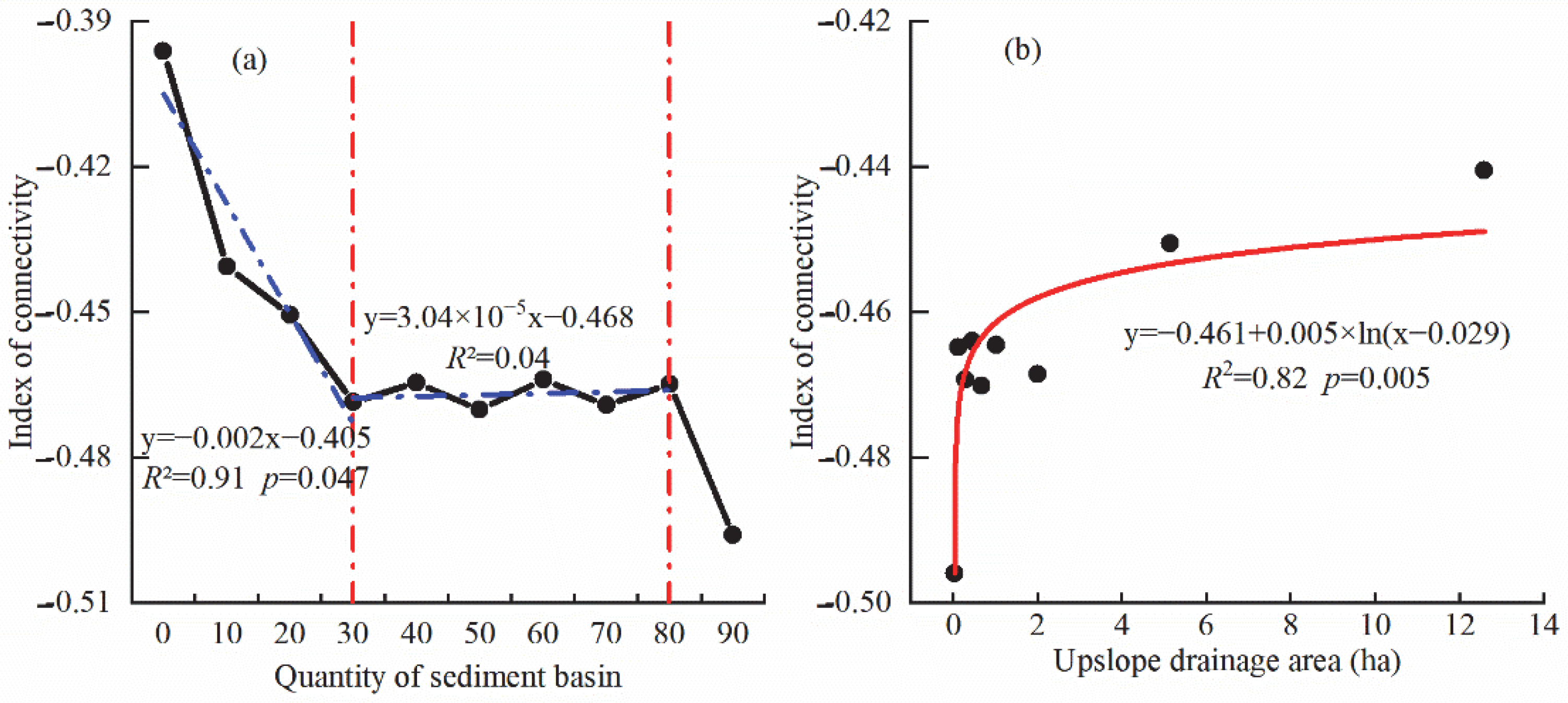
3.3. Effects of Sediment Basin on Spatial Distribution of Sediment Connectivity

The IC values, which represent sediment connectivity in this study, tended to decrease when the number of sediment basin increased from 0 to 90 (Figure 7a) and as the upslope drainage area decreased from 12.59 to 0.03 ha (Figure 7b). For example, when we compared the scenarios of zero sediments basins (Sink_0) to 90 sediment basins (Sink_90), the mean IC decreased from –0.396 to –0.496 (25.3%). This decrease highlights how effectively sediment basins reduce sediment connectivity. While this scenario represented the largest sediment connectivity reduction that could be achieved in this watershed and it assumed that the sediment basins were able to intercept 100% of sediment, it still demonstrated that sediment basins can reduce the sediment connectivity.

In scenarios with less than 30 sediment basins (where the drainage area of the road segments’ upslope watersheds was 1.99–12.59 ha), when the number of sediment basins increased or the upslope drainage area decreased, the sediment connectivity of the Xiangchagou watershed significantly decreased (p < 0.05). By contrast, when the number of sediment basins increased from 30 to 80 (the upslope drainage area of the road segments decreased from 1.99 to 0.11 ha), the sediment connectivity hardly changed. This indicated that when the threshold upslope drainage area of road segments decreased to a certain range, increasing the number of sediment basins did not significantly affect sediment connectivity. Therefore, IC was not proportional to the number of sediment basins. So, although installing the maximum number of sediment basins (Sink_90) reduced the road segments’ upslope watershed area to 0.03 ha, which decreased the sediment connectivity of the Xiangchagou watershed, this scenario was unrealistic. The high financial and ecological cost (in terms of forest disturbance) creates an imperative to determine the optimal number of sediment basins and threshold of upslope drainage area.

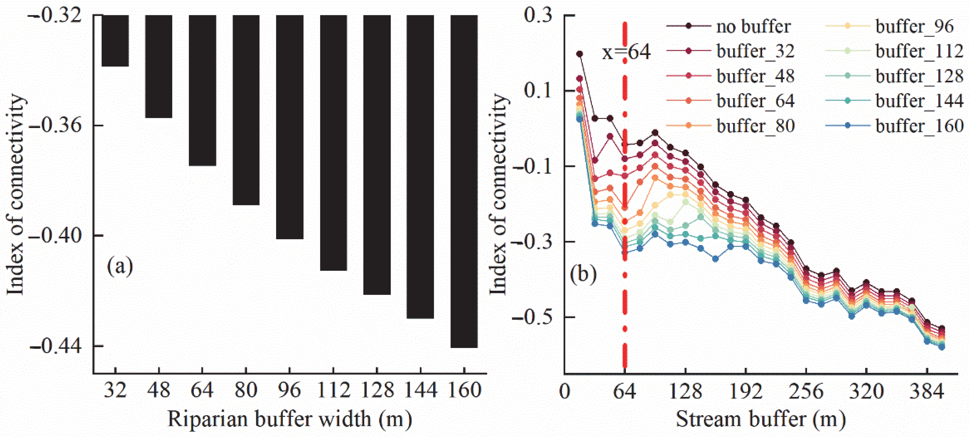
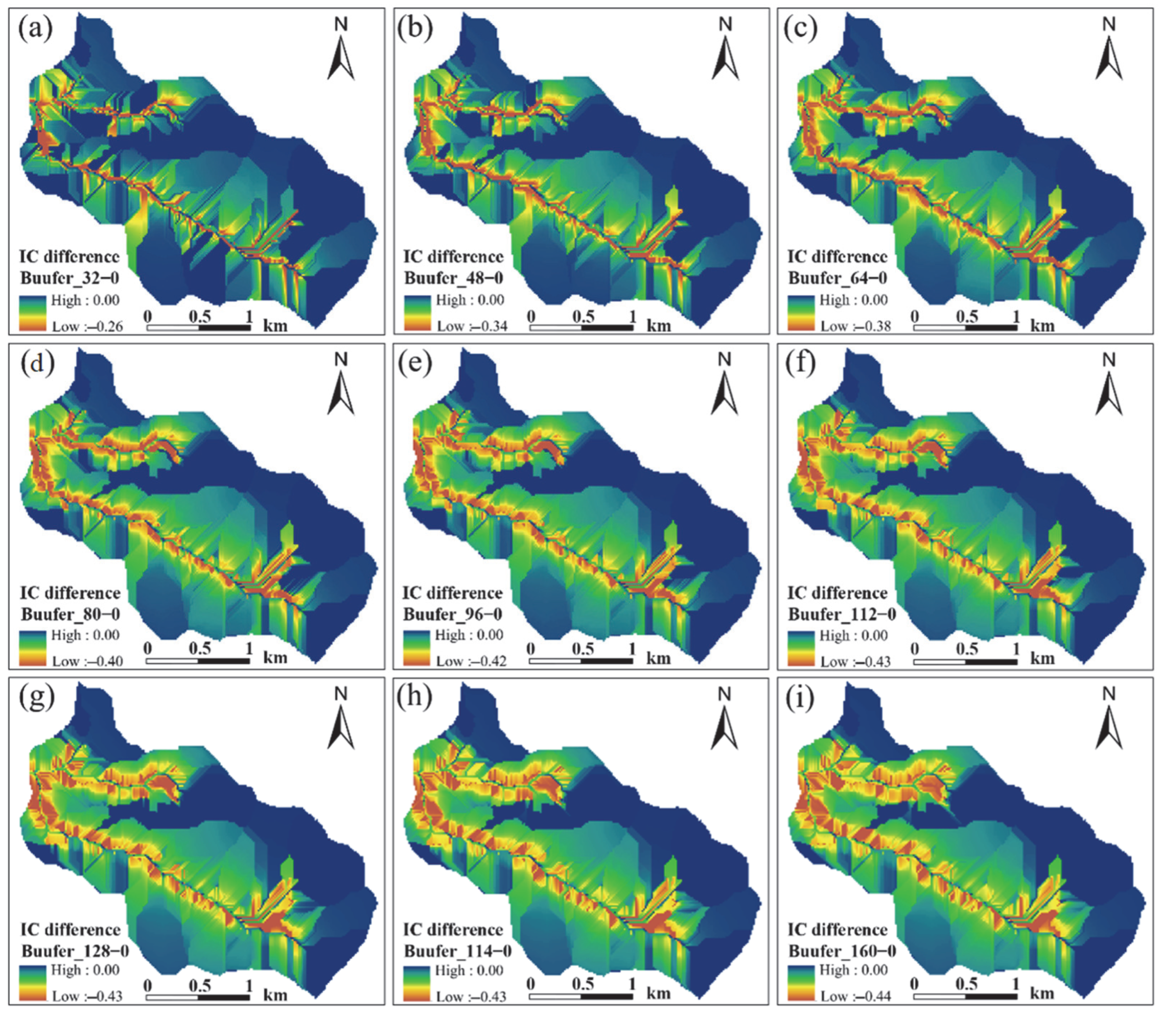
3.4. Effects of Riparian Buffer on Spatial Distribution of Sediment Connectivity

Figure 8 shows effect of riparian buffer widths on IC values for the Xiangchagou watershed and how these values vary based on their distance from streams. The IC values ranged from 3.20 (low) to 3.35 (high), and sediment connectivity generally decreased linearly as both riparian buffer width (Figure 8a) and distance to stream (Figure 8b) increased. Note that sediment connectivity decreased sharply when riparian buffer widths were in the 0–64 m zones, whereas sediment connectivity rose and fell when riparian buffers were within the 64–160 m zones. Sediment connectivity likely increased in the 64–96 m zones because the riparian buffers were adjacent to roads and streams (Figure 5). Figure 9 presents the difference of sediment connectivity under different riparian buffer scenarios from that without riparian buffers. Comparing these scenarios to the absence of a riparian buffer, the mean IC values of buffer_32 to buffer_160 decreased by 0.020 to 0.121. That is, increasing the buffer width caused greater reductions in IC compared to not having a riparian buffer. Moreover, within this range of values, as the distance between the riparian buffer and stream increased, the marginal value of IC for each buffer width decreased, meaning that IC did not increase proportionally to the width of the riparian buffer when the buffer width was above 32 m.

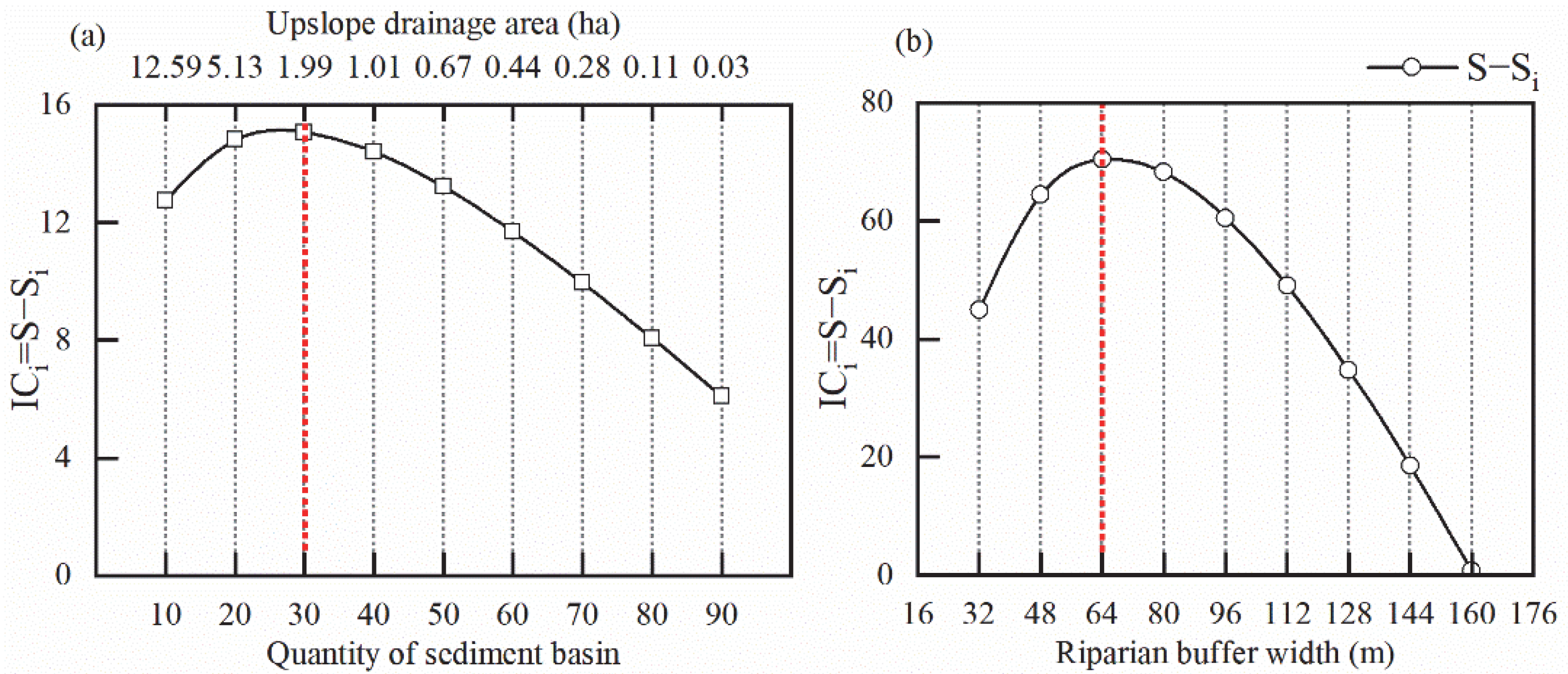
3.5. Determining Optimal Best Management Practices

Based on how IC changed with the number of sediment basins and the width of riparian buffers, we were able to draw variation curves using the mean change point method for the difference between S and S_i (S − S_i) of the number of sediment basins and riparian buffer width. For the sediment basin scenarios (Figure 10a), S − S_i was greatest when there were 30 sediment basins and the corresponding road segments’ upslope drainage areas were 2 ha. For the riparian buffer scenarios (Figure 10b), S − S_i was greatest when the riparian buffer width was 64 m. Accordingly, we could improve sediment connectivity the most in the Xiangchagou watershed if we implemented (1) 30 sediment basins at forest roads and (2) a riparian buffer 64 m wide. Furthermore, these data indicated that sediment basins should be installed when a road segment’s upslope drainage area is greater than 2 ha. These recommendations pertain to the present study area and to topographically similar watersheds.

4. Discussion

4.1. Road–Stream Relationship Influence Sediment Connectivity

Forest roads can significantly increase the sediment connectivity of a watershed when they intercept eroded sediment [12] because roads act as sediment transport pathways, changing the direction and convergence of sediment [9]. This is because roads develop channelized flow pathways and gullies, which carry surface and subsurface flow, transporting and discharging more sediment at the topographical or engineered drains and road–stream crossings than would occur otherwise [11,20]. Furthermore, when roads and streams intercept (“road–stream crossings”), they create a major point for sediment to enter from roads to streams [41], dramatically increasing sediment connectivity from hillslopes to the streams [26,31,39] and producing and delivering eroded sediments [11,24]. As such, road–stream connectivity is an important mode of carrying sediment downstream, and forest management measures are needed to control road erosion by targeting roads in close proximity to streams and reducing the sediment connectivity between roads and streams. Best management practices that accomplish these goals have been used in many forest management strategies to mitigate the effects of forest roads on sediment connectivity [30,46].

Previous studies calculating IC have not fully considered how roads alter the direction and pathways of overland flow because they lacked high-resolution topographic data [47], especially in large watersheds [48], and thus have underestimated sediment connectivity. Our study confirmed the influence of road–stream crossings on sediment connectivity by demonstrating that IC values were greater near road–stream crossings than at forest roads and streams with the same buffer distance. Furthermore, these relationships are greatly influenced by the spatial distribution of (proximity between) roads and streams [30]. Our data demonstrated that these phenomena similarly hold true for sediment connectivity in the Xiangchagou watershed. Our data revealed that roads and streams often occur near each other: frequency distributions indicated that roads and streams largely exist within 180 m of each other. Stream buffers with greater road densities tended to have larger IC values and, accordingly, more opportunities to deliver eroded sediment from roads to streams. Other studies have similarly found that the greatest drainage density occurred 50–100 ft (15.24–30.48 m) from streams within a watershed because roads were nearby [46]. Accordingly, our study was in agreement with existing literature indicating that a road’s proximity to a stream increases sediment connectivity, thus increasing the proportion of road-eroded sediment delivered to streams [30].

Forest management to implement BMPs, such as sediment basins and riparian buffers, at road segments and stream most in need of them require technologies to rapidly assess sediment production and delivery [30]. However, in the absence of long-term field monitoring on sediment production and delivery, it is difficult to provide this assessment. Therefore, we used IC as a shorthand for sediment connectivity and assessed how the values were affected by different scenarios of implementing sediment basins and riparian buffer. Using IC as a shorthand helped to quickly determine the likelihood of a watershed to produce and deliver sediment [15,38], and it revealed the locations with the greatest potential to reduce sediment delivery in the watershed [30]. We then combined this information with scenarios based off of various BMP deployment scenarios to determine an optimal strategy to mitigate the most sediment loss with the least BMPs [49]. In this study, we used forest roads as drainage pathways and local sinks for eroded sediments, and then, we calculated IC by incorporating roads into its calculation processes based on mesoscale resolution DEM. By doing this, we were able to more precisely present solutions to decrease sediment connectivity along roads [50].

4.2. Optimization of Forest Management Measures

This study provides clear evidence that installing sediment basin and riparian buffers can effectively decrease the sediment connectivity between roads and streams in a watershed. Specifically, in the Xiangchagou watershed, adding the maximum number of sediment basins (90) decreased the mean IC value by 19.78% compared to an absence of sediment basins (the current condition). This is likely because frequently draining and silting sediment-loaded runoff increases sediment detention and erosion protection [1,22]. Additionally, riparian buffers in our study similarly reduced sediment transport to streams, especially as the buffer width and distance to streams increased, which is consistent with previous studies [25,44].

In contrast to previous studies, we identified specific locations and determined the optimal quantity/width of BMPs to be implemented, which increases the effectiveness of BMP implementation [30,31]. We did this by using the mean change point method to find the optimal riparian buffer width and sediment basin, and we found that in the Xiangchagou watershed, the optimal number of sediment basins is 30 and the optimal width of riparian buffers is 64 m. Specifically, priority should be given to installing the optimal number of sediment basins because they are more effective at reducing sediment connectivity compared to riparian buffers. Lastly, we determined the road segments’ minimum upslope drainage area of 2 ha in order to provide a reference for installing sediment basins on newly constructed or paved forest roads in this, or topographically similar, mountainous watersheds. It has to be noted that both the observed optimal quantity of sediment basin and the optimal width of riparian buffer are applicable to the existing forest roads in the Xiangchagou watershed, while for the existing forest road in other watersheds, it requires to be recalculated potentially according to the methodological framework proposed in this study. However, the observed road segments’ minimum upslope drainage area of 2 ha is applicable to both the existing and planning forest roads in this and the topographically similar mountainous watersheds.

4.3. Limitations and Implications

The results presented in this study help to determine optimal mitigation measures for forested roads in mountainous watersheds. However, the success of mitigation measures will vary in every watershed [31,44]. Specifically, the optimum riparian buffer width and sediment basin quantity (or minimum upslope drainage area) depends on watershed-specific factors such as soil type, slope gradient, vegetation, and topographical characteristics [39,45,51,52]. In addition to watershed characteristics, road characteristics such as road density, length, pavement type, area, and slope also influence the optimum BMPs [1,9,30]. Accordingly, this study is limited because the optimal BMPs we are recommending can only apply for this (or a very similar) watershed.

Optimum mitigation measures are context-specific, and they depend on sediment retention and connectivity, making it difficult to provide suggestion across different watersheds [24,44,53]. Furthermore, for riparian buffer widths in particular, some studies have provided evidence to utilize fixed widths [42], while others have advocated for variable widths. In this study, we recommended a riparian buffer width of 64 m, which is a fixed width that does not account for variations in site-specific information. However, these assumptions are necessary to administer and regulate BMPs [43], particularly as they relate to water management and sediment connectivity [54,55].

The optimum width of 64 m in this study is comparable to other studies conducted in the Pacific Northwest (United States) where they calculated 50 m [54], in the Mill River watershed (PEI, Canada) where they calculated 50 m [45], in the Three Gorges Reservoir area (China) where they calculated 58 m [56], and in the Little River Experimental Watershed (Georgia, USA) where they calculated 30 m [57]. These findings suggest that narrower riparian buffers with widths less than 30 m may insufficiently reduce sediment connectivity [43].

Moreover, our study assumed 100% retention efficiency in the sediment basins and that our riparian buffer was dominated by trees. These assumptions are shortfalls in our study; however, the sediment retention efficiency of sediment basins and riparian buffers has been quantitatively defined in such a way that one can differentiate the impact of quantity and width on sediment connectivity. Given these restrictions, future studies should include more details about the efficiency of their BMPs [45].

In summary, most studies about the influence of forest roads on sediment connectivity are limited and tend to be overly broad, particularly for mountainous watersheds with limited data [16,43]. Because of this clear research gap, which has been defined in previous studies [24,53], our study determined riparian buffer width and sediment basin quantity (or minimum value of upslope drainage area) to decrease sediment connectivity in mountainous, forest roads. This field demands further research [31]. In spite of sparse existing data, we were able to predict the sediment connectivity between forest roads and streams to determine the optimal implementation of BMPs to reduce sediment at the watershed scale. Furthermore, we were able to provide clear recommendations for the number of sediment basins and riparian buffer width to decrease sediment connectivity in a forested, mountainous watershed. As such, this study provides a useful reference to optimize the implementation of BMPs in this setting.

5. Conclusions

This study is unique in that we used the index of connectivity (IC) to represent sediment connectivity, which allowed us to optimize the forest best management practices in a mountainous watershed. We used remote sensing data at a mesoscale resolution, and we were able to predict a relationship between sediment connectivity based on quantity of sediment basins (minimum upslope drainage area) and riparian buffer widths. Our results indicated that forest roads and streams in mountainous watershed tend to occur close to each other, and their proximity determines the spatial distribution of sediment connectivity. Specifically, IC values decrease as the buffer distance increases for forest roads, streams, and road–stream crossings. Furthermore, we found that within certain thresholds—a riparian buffer width of 64 m, 30 sediment basins, and a minimum upslope drainage area of 2 ha—sediment connectivity significantly decreases as these values increase. However, above these thresholds, increasing the riparian buffer width, quantity of sediment basins, or upslope drainage area does little to reduce sediment connectivity. Accordingly, we were able to use the mean change point method to determine that a riparian buffer width of 64 m, 30 sediment basins, and a minimum upslope drainage area of 2 ha were optimal BMPs for the Xiangchagou watershed. Therefore, this study provides a guide for forest managers and stakeholders to design and optimize BMPs to reduce sediment connectivity, and it should be built upon in future studies to determine the optimum BMPs for forest roads in a mountainous watershed. Moving forward, future work should improve these estimates by incorporating further investigation and long-term monitoring, and through conducting more high-resolution remote sensing data.

References

- Surfleet, C.G.; Marks, S.J. Hydrologic and suspended sediment effects of forest roads using field and DHSVM modelling studies. For. Ecol. Manag. 2021, 499, 119632. [Google Scholar] [CrossRef]
- Kazama, V.S.; Corte, A.P.D.; Robert, R.C.G.; Sanquetta, C.R.; Arce, J.E.; Oliveira-Nascimento, K.A.; DeArmond, D. Global review on forest road optimization planning: Support for sustainable forest management in Amazonia. For. Ecol. Manag. 2021, 492, 119159. [Google Scholar] [CrossRef]
- Cao, L.; Zhang, K.; Dai, H.; Liang, Y. Modeling interrill erosion on unpaved roads in the loess plateau of China. Land Degrad. Dev. 2015, 26, 825–832. [Google Scholar] [CrossRef]
- Dietrich, M.; O’Shea, M.J.; Gieré, R.; Krekeler, M.P.S. Road sediment, an underutilized material in environmental science research: A review of perspectives on United States studies with international context. J. Hazard. Mater. 2022, 432, 128604. [Google Scholar] [CrossRef] [PubMed]
- Ramos-Scharrón, C.E. Land disturbance effects of roads in runoff and sediment production on dry-tropical settings. Geoderma 2018, 310, 107–119. [Google Scholar] [CrossRef]
- Touma, B.R.; Kondolf, G.M.; Walls, S. Impacts of sediment derived from erosion of partially-constructed road on aquatic organisms in a tropical river: The Río San Juan, Nicaragua and Costa Rica. PLoS ONE 2020, 15, e0242356. [Google Scholar] [CrossRef]
- Locatelli, B.; Laumonier, Y.; Freycon, V.; Bernoux, M. Soil erosion in the humid tropics: A systematic quantitative review. Agric. Ecosyst. Environ. 2015, 203, 127–139. [Google Scholar] [CrossRef]
- Fidelus-Orzechowska, J.; Strzyżowski, D.; Żelazny, M. The geomorphic activity of forest roads and its dependencies in the Tatra Mountains. Geogr. Ann. Ser. A Phys. Geogr. 2018, 100, 59–74. [Google Scholar] [CrossRef]
- Jing, Y.; Zhao, Q.; Lu, M.; Wang, A.; Yu, J.; Liu, Y.; Ding, S. Effects of road and river networks on sediment connectivity in mountainous watersheds. Sci. Total Environ. 2022, 826, 154189. [Google Scholar] [CrossRef]
- Farias, T.R.L.; Medeiros, P.H.A.; de Araújo, J.C.; Navarro-Hevia, J. The role of unpaved roads in the sediment budget of a semiarid mesoscale catchment. Land Degrad. Dev. 2021, 32, 5443–5454. [Google Scholar] [CrossRef]
- Ramos-Scharrón, C.E. Impacts of off-road vehicle tracks on runoff, erosion and sediment delivery—A combined field and modeling approach. Environ. Model. Softw. 2021, 136, 104957. [Google Scholar] [CrossRef]
- Zhao, Q.; Jing, Y.; Wang, A.; Yu, Z.; Liu, Y.; Yu, J.; Liu, G.; Ding, S. Response of sediment connectivity to altered convergence processes induced by forest roads in mountainous watershed. Remote Sens. 2022, 14, 3603. Available online: https://www.mdpi.com/2072-4292/14/15/3603 (accessed on 22 August 2022). [CrossRef]
- Guo, W.; Bai, Y.; Cui, Z.; Wang, W.; Li, J.; Su, Z. The impact of concentrated flow and slope on unpaved loess-road erosion on the Chinese Loess Plateau. Land Degrad. Dev. 2021, 32, 914–925. [Google Scholar] [CrossRef]
- Zhao, Q.; Zhang, Y.; Xu, S.; Ji, X.; Wang, S.; Ding, S. Relationships between riparian vegetation pattern and the hydraulic characteristics of upslope runoff. Sustainability 2019, 11, 2966. Available online: https://www.mdpi.com/2071-1050/11/10/2966 (accessed on 22 August 2022). [CrossRef]
- Hernani, H. Application of LiDAR DEM Metrics to Estimate Road-Stream Sediment Connectivity in Alberta Eastslopes Salmonid Habitats. Master’s Thesis, University of Alberta, Edmonton, AB, Canada, 2019. [Google Scholar] [CrossRef]
- Sosa-Pérez, G.; MacDonald, L.H. Reductions in road sediment production and road-stream connectivity from two decommissioning treatments. For. Ecol. Manag. 2017, 398, 116–129. [Google Scholar] [CrossRef]
- Llena, M.; Vericat, D.; Cavalli, M.; Crema, S.; Smith, M.W. The effects of land use and topographic changes on sediment connectivity in mountain catchments. Sci. Total Environ. 2019, 660, 899–912. [Google Scholar] [CrossRef]
- Roy, S.; Sahu, A.S. Potential interaction between transport and stream networks over the lowland rivers in Eastern India. J. Environ. Manag. 2017, 197, 316–330. [Google Scholar] [CrossRef]
- Wemple, B.C.; Jones, J.A.; Grant, G.E. Channel network extension by logging roads in two basins, Western Cascades, Oregon. J. Am. Water Resour. Assoc. 1996, 32, 1195–1207. [Google Scholar] [CrossRef]
- Fu, B.; Newham, L.T.; Ramos-Scharron, C. A review of surface erosion and sediment delivery models for unsealed roads. Environ. Model. Softw. 2010, 25, 1–14. [Google Scholar] [CrossRef]
- Eisenbies, M.; Aust, W.; Burger, J.; Adams, M.B. Forest operations, extreme flooding events, and considerations for hydrologic modeling in the Appalachians—A review. For. Ecol. Manag. 2007, 242, 77–98. [Google Scholar] [CrossRef]
- Sosa-Pérez, G.; MacDonald, L. Wildfire effects on road surface erosion, deposition, and road–stream connectivity. Earth Surf. Process. Landf. 2017, 42, 735–748. [Google Scholar] [CrossRef]
- Persichillo, M.G.; Bordoni, M.; Cavalli, M.; Crema, S.; Meisina, C. The role of human activities on sediment connectivity of shallow landslides. Catena 2018, 160, 261–274. [Google Scholar] [CrossRef]
- Lang, A.J.; Aust, W.M.; Bolding, M.C.; McGuire, K.J.; Schilling, E.B. Best management practices influence sediment delivery from road stream crossings to mountain and piedmont streams. For. Sci. 2018, 64, 682–695. [Google Scholar] [CrossRef]
- Rachels, A.A.; Bladon, K.D.; Bywater-Reyes, S.; Hatten, J.A. Quantifying effects of forest harvesting on sources of suspended sediment to an Oregon Coast Range headwater stream. For. Ecol. Manag. 2020, 466, 118123. [Google Scholar] [CrossRef]
- Dangle, C.; Bolding, M.; Aust, W.; Barrett, S.; Schilling, E. Best management practices influence modeled erosion rates at forest haul road stream crossings in Virginia. J. Am. Water Resour. Assoc. 2019, 55, 1169–1182. [Google Scholar] [CrossRef]
- Lu, M.; Zhao, Q.; Ding, S.; Wang, S.; Hong, Z.; Jing, Y.; Wang, A. Hydro-geomorphological characteristics in response to the water-sediment regulation scheme of the Xiaolangdi Dam in the lower Yellow River. J. Clean. Prod. 2022, 335, 130324. [Google Scholar] [CrossRef]
- Solgi, A.; Naghdi, R.; Zenner, E.K.; Hemmati, V.; Behjou, F.K.; Masumian, A. Evaluating the effectiveness of mulching for reducing soil erosion in cut slope and fill slope of forest roads in Hyrcanian forests. Croat. J. For. Eng. 2021, 42, 259–268. [Google Scholar] [CrossRef]
- Luo, H.; Zhao, T.; Dong, M.; Gao, J.; Peng, X.; Guo, Y.; Wang, Z.; Liang, C. Field studies on the effects of three geotextiles on runoff and erosion of road slope in Beijing, China. Catena 2013, 109, 150–156. [Google Scholar] [CrossRef]
- Benda, L.; James, C.; Miller, D.; Andras, K. Road Erosion and Delivery Index (READI): A model for evaluating unpaved road erosion and stream sediment delivery. J. Am. Water Resour. Assoc. 2019, 55, 459–484. [Google Scholar] [CrossRef]
- Lin, H.-Y.; Robinson, K.F.; Walter, L. Trade–offs among road–stream crossing upgrade prioritizations based on connectivity restoration and erosion risk control. River Res. Appl. 2020, 36, 371–382. [Google Scholar] [CrossRef]
- Ramos-Scharrón, C.E.; LaFevor, M.C. Effects of forest roads on runoff initiation in low-order ephemeral streams. Water Resour. Res. 2018, 54, 8613–8631. [Google Scholar] [CrossRef]
- Fressard, M.; Cossart, E. A graph theory tool for assessing structural sediment connectivity: Development and application in the Mercurey vineyards (France). Sci. Total Environ. 2019, 651, 2566–2584. [Google Scholar] [CrossRef] [PubMed]
- Thompson, C.; Hicks, A.; Sun, X. A GIS tool for the design and assessment of road drain spacing to minimize stream pollution: RoadCAT. In Proceedings of the 19th International Congress on Modelling and Simulation, Perth, Australia, 12–16 December 2011; pp. 1923–1929. Available online: http://hdl.handle.net/1885/62462 (accessed on 22 August 2022).
- Mayor, Á.G.; Bautista, S.; Small, E.E.; Dixon, M.; Bellot, J. Measurement of the connectivity of runoff source areas as determined by vegetation pattern and topography: A tool for assessing potential water and soil losses in drylands. Water Resour. Res. 2008, 44, W10423. [Google Scholar] [CrossRef]
- Zingaro, M.; Refice, A.; Giachetta, E.; D’Addabbo, A.; Lovergine, F.; De Pasquale, V.; Pepe, G.; Brandolini, P.; Cevasco, A.; Capolongo, D. Sediment mobility and connectivity in a catchment: A new mapping approach. Sci. Total Environ. 2019, 672, 763–775. [Google Scholar] [CrossRef] [PubMed]
- Borselli, L.; Cassi, P.; Torri, D. Prolegomena to sediment and flow connectivity in the landscape: A GIS and field numerical assessment. Catena 2008, 75, 268–277. [Google Scholar] [CrossRef]
- Zanandrea, F.; Michel, G.P.; Kobiyama, M. Impedance influence on the index of sediment connectivity in a forested mountainous catchment. Geomorphology 2020, 351, 106962. [Google Scholar] [CrossRef]
- Thomaz, E.L.; Peretto, G.T. Hydrogeomorphic connectivity on roads crossing in rural headwaters and its effect on stream dynamics. Sci. Total Environ. 2016, 550, 547–555. [Google Scholar] [CrossRef]
- Kalantari, Z.; Cavalli, M.; Cantone, C.; Crema, S.; Destouni, G. Flood probability quantification for road infrastructure: Data-driven spatial-statistical approach and case study applications. Sci. Total Environ. 2017, 581–582, 386–398. [Google Scholar] [CrossRef]
- Lang, A.J.; Aust, W.M.; Bolding, M.C.; Mcguire, K.J.; Schilling, E.B. Comparing sediment trap data with erosion models for evaluation of forest haul road stream crossing approaches. Trans. Asae Am. Soc. Agric. Eng. 2017, 60, 393–408. [Google Scholar] [CrossRef]
- Kuglerová, L.; Jyväsjärvi, J.; Ruffing, C.; Muotka, T.; Jonsson, A.; Andersson, E.; Richardson, J.S. Cutting edge: A comparison of contemporary practices of riparian buffer retention around small streams in Canada, Finland, and Sweden. Water Resour. Res. 2020, 56, e2019WR026381. [Google Scholar] [CrossRef]
- Arif, M.; Tahir, M.; Jie, Z.; Changxiao, L. Impacts of riparian width and stream channel width on ecological networks in main waterways and tributaries. Sci. Total Environ. 2021, 792, 148457. [Google Scholar] [CrossRef] [PubMed]
- Cole, L.J.; Stockan, J.; Helliwell, R. Managing riparian buffer strips to optimise ecosystem services: A review. Agric. Ecosyst. Environ. 2020, 296, 106891. [Google Scholar] [CrossRef]
- Sirabahenda, Z.; St-Hilaire, A.; Courtenay, S.C.; van den Heuvel, M.R. Assessment of the effective width of riparian buffer strips to reduce suspended sediment in an agricultural landscape using ANFIS and SWAT models. Catena 2020, 195, 104762. [Google Scholar] [CrossRef]
- Dutton, P.D. Factors Influencing Roadside Erosion and In-Stream Geomorphic Stability at Road-Stream Crossings for Selected Watersheds, North Shore, Minnesota, USA. Ph.D. Thesis, University of Minnesota, Minneapolis, MN, USA, 2012. Available online: https://hdl.handle.net/11299/140028 (accessed on 22 August 2022).
- López-Vicente, M.; González-Romero, J.; Lucas-Borja, M.E. Forest fire effects on sediment connectivity in headwater sub-catchments: Evaluation of indices performance. Sci. Total Environ. 2020, 732, 139206. [Google Scholar] [CrossRef] [PubMed]
- Zhao, G.; Gao, P.; Tian, P.; Sun, W.; Hu, J.; Mu, X. Assessing sediment connectivity and soil erosion by water in a representative catchment on the Loess Plateau, China. Catena 2020, 185, 104284. [Google Scholar] [CrossRef]
- Seutloali, K.E.; Beckedahl, H.R. A review of road-related soil erosion: An assessment of causes, evaluation techniques and available control measures. Earth Sci. Res. J. 2015, 19, 73–80. [Google Scholar] [CrossRef]
- Fidelus-Orzechowska, J.; Strzyżowski, D.; Cebulski, J.; Wrońska-Wałach, D. A quantitative analysis of surface changes on an abandoned forest road in the Lejowa Valley (Tatra Mountains, Poland). Remote Sens. 2020, 12, 3467. [Google Scholar] [CrossRef]
- Xu, S.; Zhao, Q.; Liu, Y.; Ding, S.; Qin, M. Sensitivity and applicability of landscape leakiness index in determining soil and water conservation function of a subtropical riparian vegetation buffer zone. Environ. Eng. Sci. 2018, 36, 227–236. [Google Scholar] [CrossRef]
- Zhao, Q.; Ding, S.; Hong, Z.; Ji, X.; Wang, S.; Lu, M.; Jing, Y. Impacts of water-sediment regulation on spatial-temporal variations of heavy metals in riparian sediments along the middle and lower reaches of the Yellow River. Ecotoxicol. Environ. Saf. 2021, 227, 112943. [Google Scholar] [CrossRef]
- Anderson, C.J.; Lockaby, B.G. Research gaps related to forest management and stream sediment in the United States. Environ. Manag. 2011, 47, 303–313. [Google Scholar] [CrossRef]
- Stutter, M.; Costa, F.B.; Ó Uallacháin, D. The interactions of site-specific factors on riparian buffer effectiveness across multiple pollutants: A review. Sci. Total Environ. 2021, 798, 149238. [Google Scholar] [CrossRef] [PubMed]
- Zhao, Q.; Ding, S.; Lu, X.; Liang, G.; Hong, Z.; Lu, M.; Jing, Y. Water-sediment regulation scheme of the Xiaolangdi Dam influences redistribution and accumulation of heavy metals in sediments in the middle and lower reaches of the Yellow River. Catena 2022, 210, 105880. [Google Scholar] [CrossRef]
- Shan, N.; Ruan, X.-H.; Xu, J.; Pan, Z.-R. Estimating the optimal width of buffer strip for nonpoint source pollution control in the Three Gorges Reservoir Area, China. Ecol. Model. 2014, 276, 51–63. [Google Scholar] [CrossRef]
- Cho, J.; Lowrance, R.R.; Bosch, D.D.; Strickland, T.C.; Her, Y.; Vellidis, G. Effect of watershed subdivision and filter width on SWAT simulation of a coastal plain watershed. J. Am. Water Resour. Assoc. 2010, 46, 586–602. [Google Scholar] [CrossRef]