CD-SDN: Unsupervised Sensitivity Disparity Networks for Hyper-Spectral Image Change Detection

Abstract

Deep neural networks (DNNs) could be affected by the regression level of learning frameworks and challenging changes caused by external factors; their deep expressiveness is greatly restricted. Inspired by the fine-tuned DNNs with sensitivity disparity to the pixels of two states, in this paper, we propose a novel change detection scheme served by sensitivity disparity networks (CD-SDN). The CD-SDN is proposed for detecting changes in bi-temporal hyper-spectral images captured by the AVIRIS sensor and HYPERION sensor over time. In the CD-SDN, two deep learning frameworks, unchanged sensitivity network (USNet) and changed sensitivity network (CSNet), are utilized as the dominant part for the generation of binary argument map (BAM) and high assurance map (HAM). Then two approaches, arithmetic mean and argument learning, are employed to re-estimate the changes of BAM. Finally, the detected results are merged with HAM and obtain the final detected binary change maps (BCMs). Experiments are performed on three real-world hyperspectral image datasets, and the results indicate the good universality and adaptability of the proposed scheme, as well as its superiority over other existing state-of-the-art algorithms.

1. Introduction

The change detection techniques for remote sensing images usually refer to the visual presentation and quantitative analysis of change region between two scene images, which are obtained through airborne and spaceborne photography across time in the same geographical location. The two scene images consist of a reference image taken in a former time and a query image captured in the aftertime. The hyperspectral image change detection is highly applied in intelligent scenes [1,2,3], including natural disasters, pollution discharge, variations in waters and vegetation, as well as hyperspectral image classification [4,5], image recognition [6], urban planning [7], etc. The above application scenarios fully indicate the significance of this subject.

At present, algebraic operation methods still dominate the area of remote sensing image change detection. They have several competencies over the other algorithms, including simplicity and high performance to save time and space. And especially, the change vector analysis (CVA) [8] and principal component analysis (PCA) [9] are undoubtedly two classic milestones in this field. CVA is customarily used to analyze the vector increment of bi-temporal images, while PCA takes the role of a pan-sharpening algorithm to enhance the geospatial features of panchromatic, and hyperspectral images. Although the algebraic operation methods have obvious advantages in some respects, their defects and deficiencies are also quite prominent. In fact, the detected bi-temporal images normally cover a period of a long time, therefore, the natural disturbance features originating from radiometric distortion, imaging angle, variability of lighting and atmosphere, etc., will cause negative effects on the algebraic operation. It is in these circumstances that to analyze and calculate more accurate results, geometric correction [10], radiometric correction [11,12], as well as preprocessing of noise suppression/feature enhancement, etc., should be carried out in advance. Nevertheless, many of those efforts do not work well to attain the anticipant results, and change detection still faces great challenges.

In recent years, more DNNs have demonstrated their robustness of expressiveness to conquer the difficulties caused by external interferences. With respect to the simulation training of neural networks, the learning parameters generated by gradient-adjusting could reach an advanced regression level of the mathematics model, with image noises restraining to a certain extent. Apparently, DNNs perform particularly well in this regard, compared to the algebraic operation methods. Although machine learning has incomparable advantages in change detection of various real scenarios, its deep expressiveness is subject to many limitations, e.g., the disturbance of noises and, especially the sampling strategies. In the last few years, plenty of literature [13,14,15,16,17,18,19] indicates that DNN has become a hot spot in change detection. To the best of our knowledge, there are no existing works using two DNNs with sensitivity disparity to generate argument regions for further analysis.

Before discussing the employed sensitivity disparity networks (SDN), as the progressive outcome of machine learning, DNN embodies significantly less interpretability in comparison to that of traditional algorithms; and no general extraction rules exist, in terms of sampling strategy; moreover, whether to build a deep network or set hyperparameters, it largely depends on practical experience. More positively, we draw lessons from a large number of tests as, based on fully connected networks (FCN) [20], two rounds of learning parameters in the second hidden layer make the unchanged sensitivity network (USNet) more conducive, and achieve higher detection accuracy to unchanged pixels; while the opposite effect will be achieved by recycling the parameters twice in the first hidden layer, and thus to construct the changed sensitivity network (CSNet). The heterogeneous networks with sensitivity disparity act as SDN for detecting the changes of bi-temporal images, to which there will inevitably be an argument region. Thus, the re-estimating work in this region has become our new research topic. Accordingly, in this paper, we proposed the SDN, consisting of a USNet and a CSNet, to serve our proposal. Of which, according to the requirement of SDN, the PRN [21] in our last work is employed as USNet; CSNet was first proposed from the fine-tuning of FCN used in model DSFA, it has better sensitivity to changed pixels, compared with USNet. It should be noted that CD-FCN, CD-USNet, and CD-CSNet are models based on deep USNet and CSNet; although SDN contains both USNet and CSNet, this paper mainly proposes the schema CD-SDN, while the models CD-USNet and CD-CSNet with USNet and CSNet are regarded as comparison methods. In addition, the SDN was first proposed to generate the argument region. We carry out SDN to generate the binary change map (BCM) related to USNet and CSNet, respectively, denoted as USNet-BCM and CSNet-BCM. Next, High-Gain is applied to the acquired BCMs to compute the binary argument map (BAM) and high assurance map (HAM). Since the HAM is highly trusted, further analysis of changes in the scope of BAM becomes the main task. Therefore, two approaches, arithmetic mean (AM) and argument learning (AL), are then employed to produce the corresponding binary change maps, AM-BCM and AL-BCM. Finally, we merge the two re-estimated BCMs, with HAM to obtain the final detected BCMs.

2. Related Work

Generally, the current requests for change detection are mainly reflected as follows. (1) the limited photo-interpretation techniques have met the needs with difficulties to identify the large-scale image data; (2) multi-temporal and real-time intelligent monitoring calls for dynamic extraction of the change boundary and its internal area. To overcome the urgent problems that needed to be solved, machine learning played a leading role in the practical applications of change detection. As the pioneer of deep neural networks (DNN), artificial neural networks (ANN) have demonstrated their potential in change detection for Landsat digital images, because of the more flexible and arbitrary nonlinear expressiveness, stronger robustness to missing data and noises, capacity to capture more subtle spectral information, and smaller sample size, etc. An application case is a model proposed by Pu et al. [22] in 2008, the proposal is served by ANN to detect the changes in invasive species with hyper-spectral data. The comparison results have proved that the performance of ANN is better than that of linear discriminant analysis (LDA). In the next year, Ghosh et al. [23] proposed a context-sensitive technique to detect the images acquired by Enhanced Thematic Mapper Plus (ETM+) sensor carried on the Landsat-7 satellite. To overcome the selection restrictions on different categories, the modified approach, a neural network of self-organizing feature maps (SOFM), is earmarked to serve the change detection technique of context-sensitive and unsupervised. Tested results have confirmed the effectiveness of the proposal.

In the past decades, researchers have made great efforts on a variety of DNNs for solving the change detection problems of hyperspectral imagery. A case was proposed by Huang et al. [24] in 2019. In this schema, the support tensor machine (STM) is used to serve the top layer of the proposed deep belief network (DBN). The quantified results implemented on AVIRIS, and EO-1 Hyperion data have proved the higher detection accuracy of the proposal, in comparison to the outstanding baseline methods. In the same year, Huang et al. [24] designed a deep belief network based on a third-order tensor (TRS-DBN), which may fully utilize the underlying feature change information of hyperspectral remote sensing images, optimize the organizational model, and maintain the integrity of constraints between different basic elements. The test results have confirmed that TRS-DBN features higher detection accuracy compared with the methods of similarity. In the not-so-distant future of 2021, to overcome the difficulty in coping with the high-dimensional hyperspectral images with natural complexity, a deep convolutional neural network based on semantics was proposed by Moustafa et al. [25]. The test results on three hyperspectral datasets show that, with changed and unchanged areas to be highlighted, the proposed schema demonstrates its superiority in both binary and multi-change change detection.

Recent literature published on hyperspectral image change detection based on deep learning mainly lies in the following aspects: (1) pre-processing for noise bands and high dimensionality; (2) solutions for sampling balance; (3) ways to improve the expressiveness of deep networks, such as loss functions. Despite our efforts, however, the indisputable fact is that a modeling method of a special scene may be a failure in robustness, and what we urgently require is a general method, which could invariably exceed each of two member networks with sensitivity differences and are unlimited in various scenarios. Therefore, a change detection scheme served by sensitivity disparity networks (CD-SDN) is proposed to generate the argument region that is most likely to cause robustness problems, and thus to re-estimate the changes in the argument region by using two approaches.

The rest of this paper is organized as follows. Section 3 details the process of the proposed CD-SDN demonstrated; Section 4 describes the tested datasets, the experimental results of the proposed schema, and the comparison with state-of-the-art works; In Section 5 and Section 6, we make some discussion and draw conclusions, including proposing future work, respectively.

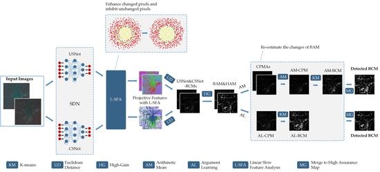
3. Materials and Methods

In preparation for the sampling strategy of the proposed change detection scheme served by sensitivity disparity networks (CD-SDN), the two-channel fully connected networks (FCN) are employed to train the bi-temporal pixels to generate the transformed features. Afterward, to get the change probability maps (CPM) and binary change map (BCM), Euclidean distance [26] and K-means [27] are applied successively. The obtained BCM serves as the reference object of sampling range for each of the tested datasets. Note that, the configuration parameters are listed in the section of the experiment; other simpler and more efficient methods such as CVA can also be used for pre-detection.

In this section, we use Figure 1 to show the flowchart of unsupervised CD-SDN and detail it as followings. (1) the SDN is initially utilized to train the model parameters with pairs of pixels selected according to the specific sampling strategies, which are detailed in the experiment section. Thereafter, two images will pass through the trained model to get the bi-temporal projective features with noise suppression; (2) linear slow feature analysis (L-SFA) [20] enhances/inhibits the changed features/unchanged features for more effective segmentation; (3) after L-SFA process, Euclidean distance is respectively employed to the projective features resulted from unchanged sensitivity network (USNet) and changed sensitivity network (CSNet), to get the USNet-CPM and CSNet-CPM, both of which are grayscale maps with a range of 0–255 to display the change degree of pixel-level; (4) K-means method serves as a threshold algorithm to the USNet-CPM and CSNet-CPM respectively, and calculates the corresponding binary change maps, USNet-BCM and CSNet-BCM, in which, the well-defined logical states 0 and 1 could uniquely determine the changes of pixel-wise; (5) High-Gain is applied on USNet-BCM and CSNet-BCM to compute the binary argument map (BAM) with non-zero gain and high assurance map (HAM) with zero gain; (6) two approaches, arithmetic mean (AM) and argument learning (AL) are utilized to re-estimate the binary changes in the BAM of interest, this inevitably generates the corresponding CPMs, on which, K-means is then utilized respectively to obtain the corresponding binary change maps, AM-BCM and AL-BCM; (7) both re-estimated BCMs are merged with HAM, and therefore generate the final detected BCMs.

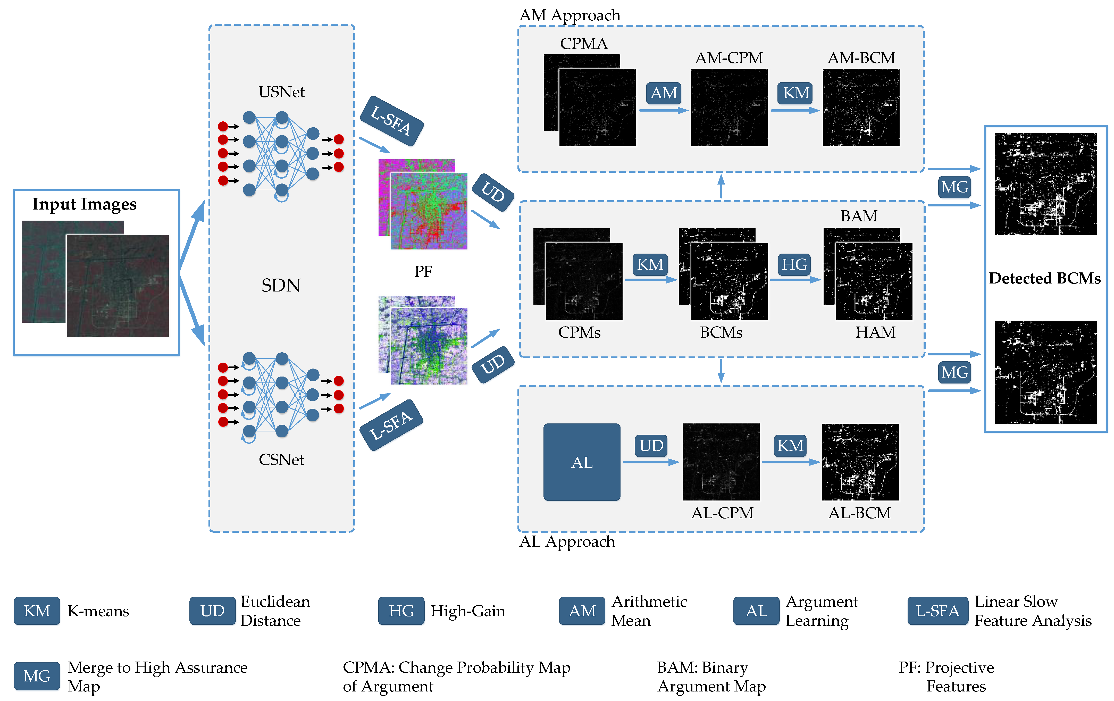
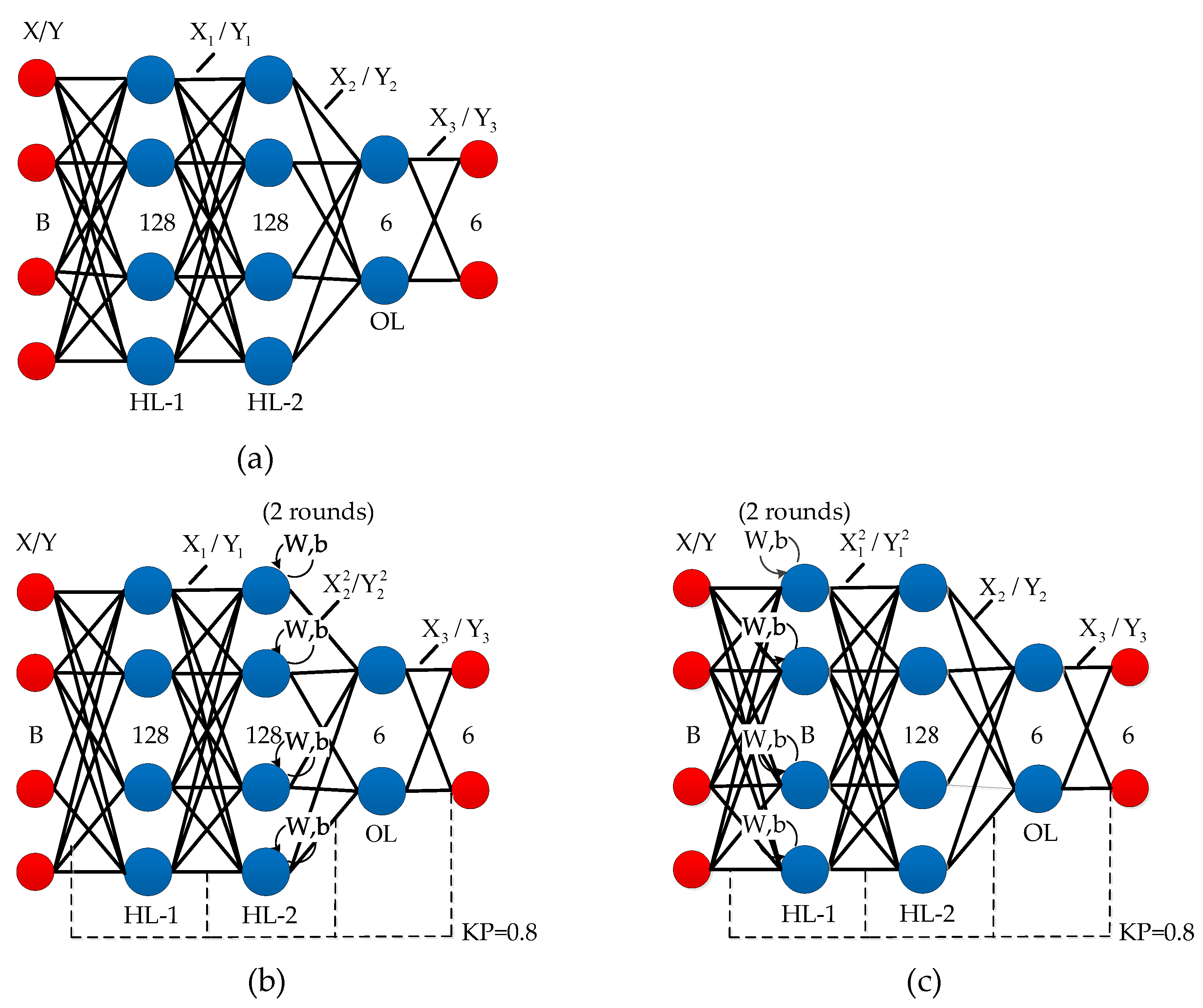
3.1. Generation of CPM & BCM

In this section, we propose SDN to learn from the bi-temporal images and generate the USNet-CPM and CSNet-CPM. Figure 2 shows the architecture of SDN composed of USNet and CSNet, as shown in Figure 2b,c respectively. Both USNet and CSNet are two-channel networks and are proposed to follow the simple two-channel FCN, as shown in Figure 2a. To facilitate the effective implementation of the networks, each image band is flattened into B one-dimensional vectors, where B represents the number of image bands. In the networks, the red-filled circles on the far left represent the input data of bi-temporal images and are denoted by X and Y; while the red-filled circles on the far right denote the projective outcome, denoted by ${\mathrm{X}}_3$ and ${\mathrm{Y}}_3$. Among the three sets of blue dots, the left two indicate the hidden layers, with the right one indicating the output layer. The acronym ‘KP’ means ‘keep probability’ and stands for the effective connection probability of nodes between two adjacent layers. The appropriate disconnection is carried out in the tests, this is helpful to improve the generalization of the training model to a certain extent.

To serve the experiment, mathematical equations of FCN are defined as (1). Based on it, the expressions of USNet and CSNet can be established as (2) and (3), respectively.

$$\begin{array}{l}{X}_1=act(W_{1,X}^{}X+b_{1,X}^{}),Y_1=act(W_{1,Y}^{}Y+b_{1,Y}^{}),\\ X_2=act(W_{2,X_1}^{}{X}_1+b_{2,X_1}^{}),Y_2=act(W_{2,Y_1}^{}{Y}_1+b_{2,Y_1}^{}),\\ X_3=act(W_{3,X_2}^{}{X}_2+b_{3,X_2}^{}),Y_3=act(W_{3,Y_2}^{}{Y}_2+b_{3,Y_2}^{}),\\ act=softsign.\end{array}$$

where $X_1/Y_1$ denotes the outcome of the first hidden layer (HL-1); while $X_2/Y_2$ indicates the computed result of the second hidden layer (HL-2); similarly, $X_3/Y_3$ represents the projective features of the output layer (OL). In the equations, ‘act’ indicates the activation function.

$$\begin{array}{l}{X}_1=ac{t}_1(W_{1,X}^{}X+b_{1,X}^{}),Y_1=ac{t}_1(W_{1,Y}^{}Y+b_{1,Y}^{}),ac{t}_1=Leaky\_Relu;\\ X_{2,1}^{}=ac{t}_2(W_{2,X_1}^{}{X}_1+b_{2,X_1}^{}),Y_{2,1}^{}=ac{t}_2(W_{2,Y_1}^{}{Y}_1+b_{2,Y_1}^{});ac{t}_2=Softsign;\\ X_{2,2}^{}=ac{t}_2(W_{2,X_1}^{}{X}_{2,1}^{}+b_{2,X_1}^{}),Y_{2,2}^{}=ac{t}_2(W_{2,Y_1}^{}{Y}_{2,1}^{}+b_{2,Y_1}^{}),ac{t}_2=Softsign;\\ X_3=ac{t}_3(W_{3,X_{2,2}^{}}^{}{X}_{2,2}^{}+b_{3,X_{2,2}^{}}^{}),Y_3=ac{t}_3(W_{3,Y_{2,2}^{}}^{}{Y}_{2,2}^{}+b_{3,Y_{2,2}^{}}^{}),ac{t}_3=tanh;\end{array}$$

The above $X_{2,1}/Y_{2,1}$ stands for the output of the first recurrence of HL-2; while $X_{2,2}/Y_{2,2}$ means the output of the second recurrence of HL-2 and the input of OL.

$$\begin{array}{l}{X}_{1,1}^{}=ac{t}_1(W_{1,X}^{}X+b_{1,X}^{}),Y_{1,1}=ac{t}_1(W_{1,Y}^{}Y+b_{1,Y}^{}),ac{t}_1=Leaky\_Relu;\\ X_{1,2}^{}=ac{t}_1(W_{1,X}^{}{X}_1+b_{1,X}^{}),Y_{1,2}^{}=ac{t}_1(W_{1,Y}^{}{Y}_1+b_{1,Y}^{}),ac{t}_1=Leaky\_Relu;\\ X_2=ac{t}_2(W_{2,X_{1,2}^{}}^{}{X}_{1,2}^{}+b_{2,X_{1,2}^{}}^{}),Y_2=ac{t}_2(W_{2,Y_{1,2}^{}}^{}{Y}_{1,2}^{}+b_{2,Y_{1,2}^{}}^{}),ac{t}_2=Softsign;\\ X_3=ac{t}_3(W_{3,X_2}^{}{X}_2+b_{3,X_2}^{}),Y_3=ac{t}_3(W_{3,Y_2}^{}{Y}_2+b_{3,Y_2}^{}),ac{t}_3=tanh;\end{array}$$

(3)

where $X_{1,1}/Y_{1,1}$ represents the output of the first recurrence of HL-1; while $X_{1,2}/Y_{1,2}$ indicates the output of the second recurrence of HL-1 and the input of HL-2.

The loss function of three networks can be mathematically expressed as (4).

$$L[(W_X,b_X),(W_Y,b_Y)]=tr[{({\widehat{B}}^{-1}\widehat{A})}^2]$$

(4)

where $W_X$, $b_X$ denote their common parameters in each layer for reference image X; while $W_Y$, $b_Y$ for query image Y. $\widehat{A}$ and $\widehat{B}$ can be expressed as (5) and (6).

$$\widehat{A}={\displaystyle \sum XY}$$

(5)

$$\widehat{B}=\frac{1}{2}({\displaystyle \sum XX+}{\displaystyle \sum YY})$$

(6)

where the ${\displaystyle \sum }XX$, ${\displaystyle \sum }YY$ and ${\displaystyle \sum }XY$ are expressed as in (22)–(24) in [20].

We feed two images across time to deep SDN for the generation of bi-temporal projective features. Then, L-SFA is employed as a difference algorithm to inhibit the unchanged pixels and enhance the changed pixels, while in the meantime, it corrects the deep features with error descriptions to a certain extent. Figure 3 shows the pixel distribution before and after L-SFA. Where the red/yellow dots indicate the changed/unchanged pixels, with a green line indicating the threshold. Before L-SFA, some red and yellow dots are on the edge of the threshold or in the opposing category, this will lead to error classification. To address this problem, the L-SFA algorithm produces a specific vector matrix, which is assigned to the bi-temporal projective features and achieves the effect as shown in Figure 3b. In addition, several noteworthy points are given as follows. First, the pixel inhibition and enhancement are not independent events, the pixels of two categories will move in opposing directions to produce a larger gap; second, L-SFA contributes to the difference of high-quality deep features, it is conducive to pixel classification, but has no supervisory behavior; third, in the case of acquiring low-quality projective features, the misdescription of pixels will be further amplified.

To solve the L-SFA problem, the following (7)–(9) are used. The core of L-SFA is the objective function and its three constraints [20]. In this case, the algebraic mapping results in a generalized eigenproblem as (7).

$$AW=BWL$$

(7)

where W denotes the generalized eigenvector matrix, while $L$ indicates the diagonal matrix of eigenvalues; A and B stand for the bi-temporal projective features of the reference image and query image, respectively, and can be calculated with the following, Equations (8) and (9).

$$A=\frac{1}{n}{\displaystyle \sum _{i=1}^n(x_i-y_i){(x_i-y_i)}^T}$$

(8)

$$B=\frac{1}{2n}({\displaystyle \sum _{i=1}^n{x}_i}{x}_i^T+{\displaystyle \sum _{i=1}^n{y}_i}{y}_i^T)$$

(9)

where $x_i$, $y_i$ denote the i-th pixel pair; while T, n represents the transpose operation of the matrix, and the number of pixels.

The calculated A and B serve (7) to obtain W. By passing the two detected images regarded as R and Q through the training model, then, we multiply the transpose of normalized W denoted by $\widehat{W}$, with bi-temporal projective features $\widehat{R}$ and $\widehat{Q}$ to produce the bi-temporal transformed features $R^{\prime }$ and $Q^{\prime }$ as (10).

$$R^{\prime }=\widehat{W}\widehat{R},Q^{\prime }=\widehat{W}\widehat{Q}.$$

(10)

When the projective features with the L-SFA algorithm are obtained, Euclidean distance [26] as (11) is used to acquire the CPM. Noted that other methods, such as Chi-square distance [28], Mahala Nobis distance [29], and Hamming/Manhattan distance [30], can also be used to calculate the CPM.

$$CPM=\sqrt{Dif{f}^{T}Diff}$$

(11)

$$Diff={\displaystyle \sum _{b=1}^B{\displaystyle \sum _{i=1}^n({\widehat{x}}_{(i,b)}-{\widehat{y}}_{(i,b)}})}$$

(12)

where “Diff” in (12) serves (11) in this work; $\widehat{x}$ and $\widehat{y}$ denote the feature units originating from the reference image and query image after L-SFA, respectively; B, b, and n respectively indicate the number of bands, the index of the band, and the number of image pixels; T denotes the transpose operation of a matrix.

We then apply K-means to the CPM, and the corresponding BCMs, USNet-BCM, and CSNet-BCM are thus generated. In the tests, the white and black marks represent the binary changed region and unchanged region, respectively.

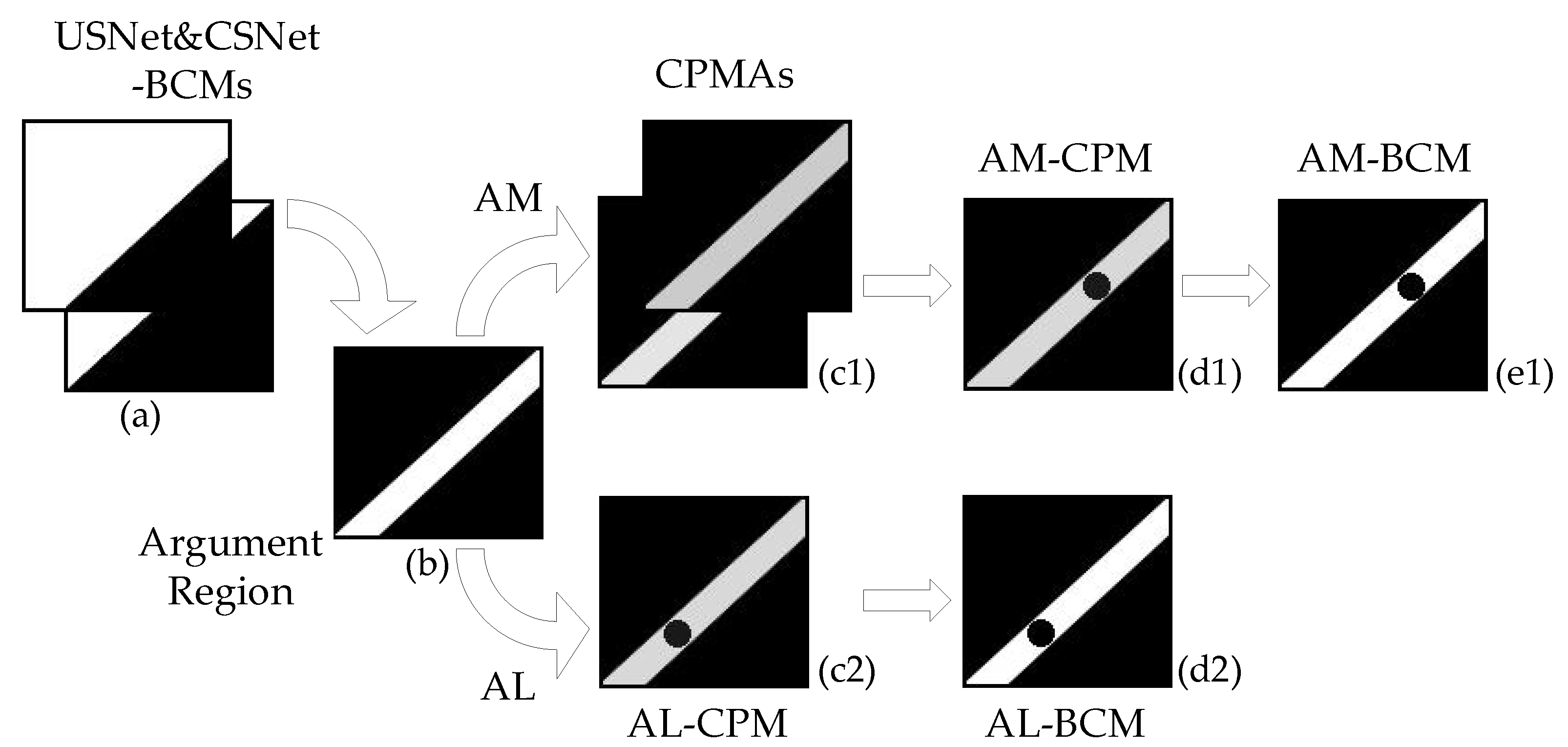
3.2. Generation of BAM & Re-Estimation of Argument Region

In this section, we first generate the BAM by using the High-Gain calculation between USNet-BCM and CSNet-BCM. In the BAM, the highlighted marks are regarded as argument regions. As we know, the HAM which lies outside the scope of BAM is easily available. After that, two approaches, AM and AL, are then employed to re-estimate the changes of BAM. Figure 4 shows the process of the two approaches. In this figure, the images of (a) signify the USNet-BCM and CSNet-BCM, in which, we mark the changed region and unchanged region with white and black, respectively; (b) shows the BAM, with white pixels representing the argument region. Thereafter, we detail the computation process of two subdivided approaches as follows.

In AM approach, we apply arithmetic mean operation to the change probability map of argument (CPMA) related to unchanged sensitivity network and changed sensitivity network, respectively, denoted as USNet-CPMA and CSNet-CPMA, as (c1) shows; to re-estimate the change probability of BAM, the obtained AM-CPM is shown as (d1). Then, K-means is used to generate the AM-BCM, displayed in (e1). In the AL approach, USNet is applied to learn from two images to be detected within the argument region. Then, Euclidean distance is utilized on bi-temporal projective features to produce the AL-CPM as (c2). Afterward, K-means is employed to segment the gray pixels of AL-CPM into binary changes reflected in AL-BCM, as shown in (d2). Finally, we merge the obtained AM-BCM and AL-BCM with HAM, and thus generate the final BCMs. The whole pseudocode of the proposed schema is summarized with Algorithm 1.

In the tests, we draw several findings of note as follows. First, it will lose significance if CD-USNet and CD-CSNet underperform in comprehensive coefficients (e.g., OA [31], Kappa, and F1 [32]); second, USNet and CSNet should have pretty remarkable sensitivity disparity to changed pixels/unchanged pixels, to produce the effective argument region; third, to generate the final detected BCM, we suggest to first transform the AM-CPM/AL-CPM into AM-BCM/AL-BCM by using K-means, as shown in Figure 5b, then merge the AM-BCM/AL-BCM with HAM shown as Figure 5c, to obtain the final detected BCM, as shown in Figure 5d; the discouraged subprocess start to obtain the combination CPM by merging the AM-CPM/AL-CPM with USNet-CPM (or CSNet-CPM), then K-means is used to generate the final detected BCM. In this circumstance, the threshold may occasionally fail to segment the AM-CPM/AL-CPM as part of the combination CPM, regarding the influence of non-argument pixels, as shown in Figure 5a.

Algorithm 1 The executive process of proposed CD-SDN to generate the final binary change map

Input: Bi-temporal images R and Q;

Output: The final binary change map BCM1 and BCM2;

1: Utilized pre-detected BCM as a reference to select training samples X and Y;

2: Initialization for parameters of SDN as ${\mathrm{A}}_{\mathrm{X}},$ ${\mathrm{A}}_{\mathrm{Y}}$;

3: while i < epochs do

4:   Compute the bi-temporal projective features of training samples:

$\hat{\mathrm{X}}$ = f (X, ${\mathrm{A}}_{\mathrm{X}},$) and $\hat{\mathrm{Y}}$ = f (Y, ${\mathrm{A}}_{\mathrm{Y}}$);

5:   Compute the gradient of Loss function $\mathrm{L}({\mathrm{A}}_{\mathrm{X}},$ ${\mathrm{A}}_{\mathrm{Y}})$ = $\mathrm{tr}[{({(\hat{\mathrm{B}})}^{-1}\hat{\mathrm{A}})}^2]$

by ∂L (${\mathrm{A}}_{\mathrm{X}},$ ${\mathrm{A}}_{\mathrm{Y}}$)/∂${\mathrm{A}}_{\mathrm{X}}$ and ∂L (${\mathrm{A}}_{\mathrm{X}},$ ${\mathrm{A}}_{\mathrm{Y}}$)/∂${\mathrm{A}}_{\mathrm{Y}}$;

6:   Update the parameters;

7:   i++;

8: end

9: Training model is used to generate the projective features $\hat{\mathrm{R}}$ and $\hat{\mathrm{Q}}$ of whole bi-temporal images R and Q;

10: Apply L-SFA to the $\hat{\mathrm{R}}$ and $\hat{\mathrm{Q}}$ for post-processing to get $\hat{\mathrm{W}}\hat{\mathrm{R}}$ and $\hat{\mathrm{W}}\hat{\mathrm{Q}}$;

11: Euclidean distance to calculate the CPM;

12: K-means to get the USNet-BCM and CSNet-BCM;

13: High-Gain to generate the BAM and HAM;

14: Case AM approach:

15:   Calculate the CPMA-USNet and CPMA-CSNet by using BAM;

16:   Arithmetic mean to get the AM-CPM;

17:   K-mean to generate the AM-BCM;

18:   Merge the AM-BCM with HAM to obtain the final BCM1;

19: Case AL approach:

20:   Argument learning to generate the projective features;

21:   Euclidean distance to calculate the AL-CPM;

22:   K-means is to generate the AL-BCM;

23:   Merge the AL-BCM with HAM to obtain the final BCM2;

24:   return BCM1, BCM2;

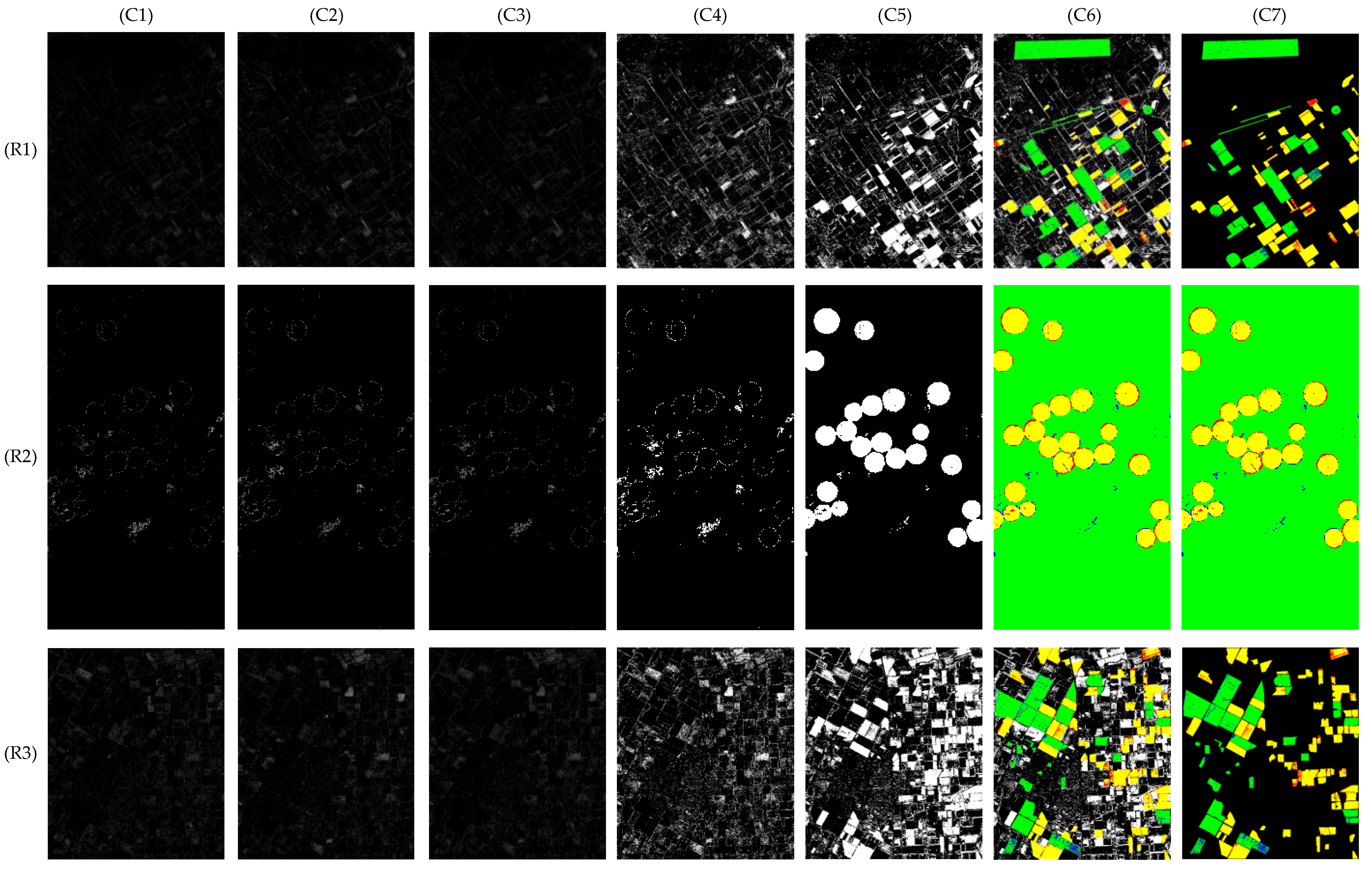
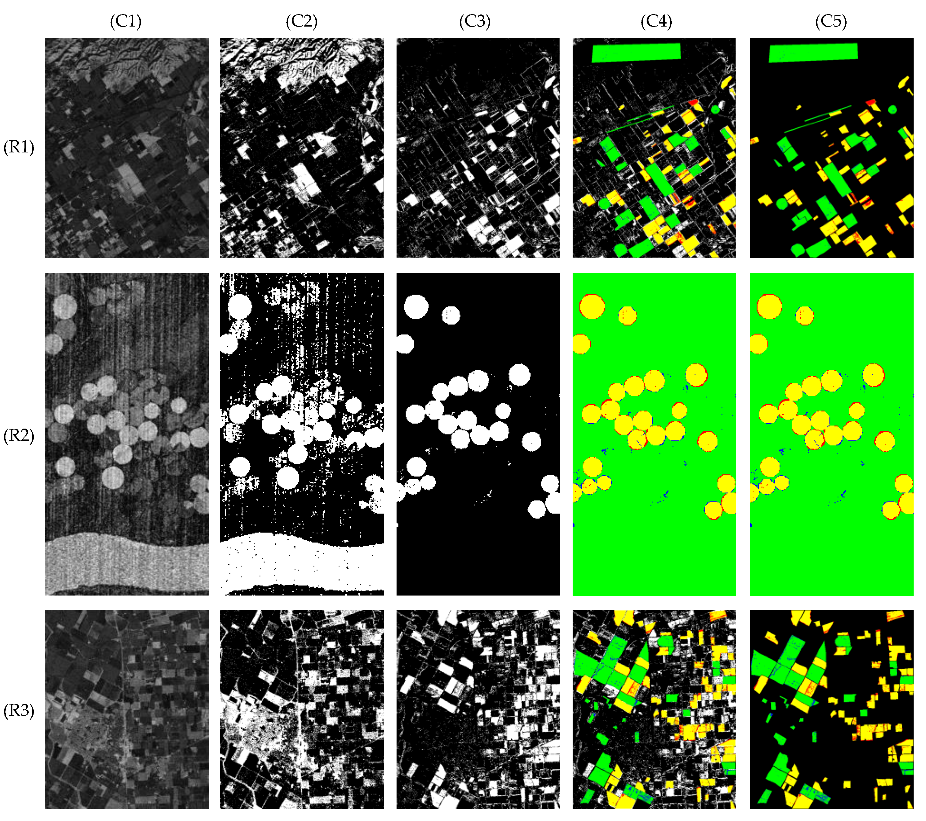
4. Results

In this section, we perform the proposed change detection scheme served by sensitivity disparity networks (CD-SDN) with three bi-temporal image datasets including ‘Santa Barbara’, ‘Hermiston’ and ‘Bay Area’, which could be acquired from the “Hyperspectral change detection dataset” [33]. The dataset ‘Santa Barbara’ contains two scene images taken over the region of Santa Barbara, California, USA, by AVIRIS sensor with 20 m ground resolution, in 2013 and 2014, with the spatial dimension of 984 × 740 × 224. In dataset ‘Hermiston’, the two images were captured by HYPERION sensor in 2004 and 2007, respectively, with 30 m ground resolution and spatial dimension of 390 × 200 × 242, over Hermiston City, Oregon. The scene images of ‘Bay Area’ were taken by AVIRIS sensor with 20m ground resolution in 2013 and 2015, respectively, over Patterson City, California, USA, with the multi-dimensional bi-temporal images expressed as 600 × 500 × 224. In three sets of spatial dimensions, the three numbers respectively indicate the height, the width, and the number of spectral bands. Figure 6(C1), (C2) and (C3) respectively list the reference images, query images, and ground truth maps of three tested datasets. In the ground truth maps of datasets ‘Santa Barbara’ and ‘Bay Area’, the white, silver, and black marks represent the changed, unchanged, and unknown regions, respectively. To ‘Santa Barbara’, each scene image contains 728,160 pixels, including 52,134 changed pixels, 80,418 unchanged pixels, and 595,608 unknown pixels; while each scene image of ‘Bay Area’ has 300,000 pixels including 39,270 changed pixels, 34,211 unchanged pixels, and 226,519 unknown pixels; Unlike the other two, the full ground truth map of ‘Hermiston’ is known, with 9986 pixels marked with white and 68,014 pixels marked with black to represent the changed region and unchanged region, respectively.

We implement the proposed CD-SDN, and evaluate the performance with five quantitative coefficients OA_CHG, OA_UN, OA [31], Kappa, and F1 [32], as defined in (13)–(17).

$$OA\_CHG=\frac{TP}{P_{kn}}$$

(13)

$$OA\_UN=\frac{TN}{N_{kn}}$$

(14)

$$OA=\frac{TP+TN}{AL{L}_{kn}}$$

(15)

$$Kappa=\frac{OA-Pe}{1-Pe},Pe=\frac{P_{kn}(TP+FP)+N_{kn}(TN+FN)}{AL{L}_{kn}^2}.$$

(16)

$$F1=\frac{2TP}{2TP+FP+FN}$$

(17)

where the two one-sided coefficients OA_CHG and OA_UN indicate the hit rate of changed pixels and unchanged pixels, respectively; while OA, Kappa, and F1 are three comprehensive coefficients. In equations, TP (true positives) and TN (true negatives) denote the number of changed pixels with a correct hit, and the number of unchanged pixels with a correct hit, respectively; $P_{kn}$ and $N_{kn}$ represent the number of changed pixels, and the number of unchanged pixels in the known region; FP (false positives) and FN (false negatives) stand for the number of changed pixels with a false hit, and the number of unchanged pixels with a false hit, respectively; $AL{L}_{kn}$ signifies the number of known pixels in the ground truth map.

4.1. Performance of Proposed CD-SDN

In Figure 6, (R1)–(R3) corresponds to the datasets ‘Santa Barbara’, ‘Hermiston’, and ‘Bay Area’, respectively. (C4)–(C7) show the change probability maps (CPM) resulting from unchanged and changed sensitivity networks, USNet-CPM and CSNet-CPM, and the binary change maps (BCM) related to USNet and CSNet, USNet-BCM, and CSNet-BCM, respectively. In (C4) and (C5), the bright regions indicate high change probability, while the dark regions indicate low change probability. To distinguish the changed pixels from the unchanged ones, the K-means clustering algorithm is then employed to generate the USNet-BCM and CSNet-BCM, as shown in (C6) and (C7), where the white marks and black marks represent the changed region and unchanged region, respectively. Accordingly, the argument region is therefore shown in (C8).

Afterward, two approaches arithmetic mean (AM) and argument learning (AL) is carried out to re-estimate the changes of (C8), and the corresponding results are shown in Figure 7 and Figure 8. In Figure 7, (C1) and (C2) respectively display the change probability map of argument (CPMA) related to unchanged sensitivity network and changed sensitivity network, USNet-CPMA, and CSNet-CPMA; (C3) shows the CPM by using AM (AM-CPM), and are generated from (C1) and (C2). Significantly, the changes of two CPMAs and AM-CPM are usually distributed near the threshold, they are not too bright or dark. There, (C4) shows the BCM by using AM (AM-BCM) obtained by using K-means on the previous image. Next, we merge AM-BCM with a high assurance map (HAM) to produce the final detected BCM, as shown in (C5). At last, (C6) corresponds to the full hitting status map (F-HSM), which represents the detected results of the known region with different colors for the full image. In F-HSM, the yellow, green, red, blue, black, and white are used to mark the correct hits to changed pixels, the correct hits to unchanged pixels, the false hits as unchanged pixels, the false hits as changed pixels, the unchanged pixels outside the known region, and the changed pixels outside the known region, respectively. However, the quantitative analysis only requires the known HSM (K-HSM), in which we cover the unknown region with black, as shown in (C7).

Figure 8 shows the results of the re-estimation process by using AL. In doing this, various excellent DNNs, such as USNet and CSNet, can be applied to this learning task. In tests, we use USNet to learn pixel pairs based on the BAM and obtain the AL projective features. Then, Euclidean distance [26] is used on the previous outcome to generate the CPM by using AL (AL-CPM) as shown in Figure 8(C1), from which we observe that, the change states of many pixels deviate from the facts, this largely results from the error projection of argument learning outside the region of interest. Yet in this stage, we can ignore it. Figure 8(C2) shows the BCM by using AL (AL-BCM). By merging the AL-BCM with HAM, the final detected BCM is obtained, as shown in (C3). It is noticeable that (C4) and (C5) demonstrate the F-HSM and K-HSM, respectively. Since the full ground truth map of dataset ‘Hermiston’ is known, the F-HSM and K-HSM are the same, as shown in Figure 7(R2,C6),(R2,C7) and Figure 8(R2,C4),(R2,C5).

4.2. Comparison with State-of-the-Art Works

To highlight the priority of the proposed CD-SDN, we compare it with the state-of-the-art works: CVA [8], CD-FCN [20], DSFA [20], CD-USNet which we proposed in our previous work and was also known in [21], and the proposed CD-CSNet. Note that in our experiment, we adopt $5\times {10}^{-5}$ as the learning rate (LR) for FCN, DSFA, USNet, and CSNet. Deep learning deserves careful considerations of LR, as follows: (1) small LR could lead to convergence difficulty of learning model; (2) large LR may result in non-convergence, faster processing speed but more memory capacity; (3) it seems almost no way but empirical rules to estimate the optimal parameters of the deep model, for a particular problem.

In network training experiments, CD-FCN pre-detection with high assurance is required. Then, based on the detected BCM resulting from CD-FCN, 3000 symmetric pixels in the changed region are selected for testing the dataset ‘Santa Barbara’, while 3000 in the unchanged region are chosen for datasets ‘Hermiston’ and ‘Bay Area’. It is emphasized especially that, the sampling strategy of dataset ‘Santa Barbara’ differs from that of the other two and, because in the tests, all DNN-based models adopt the same sampling on a specific dataset, their comparison is fair. Simultaneously, 3000/2000/2000 epochs are respectively taken to achieve the learning tasks on dataset ‘Santa Barbara’/‘Hermiston’/‘Bay Area’. But in the AL approach, 20% of argument pixels are selected as training samples; and since few pixels needed to be expressed in this phase, only 100 epochs are required.

Figure 9, Figure 10 and Figure 11 show the visualization comparison of tested results on three datasets, with (C1)–(C7) corresponding to different methods. In Figure 9 and Figure 11, (R1)–(R4) display the CPM, BCM, F-HSM, and K-HSM, respectively; while in Figure 10, (R3) shows the HSM instead of F-HSM and K-HSM because the full image of dataset ‘Hermiston’ is known. In particular, (R1,C6)-left and (R1,C7)-left are two USNet-CPMs; (R1,C6)-right indicates the AM-CPM, while (R1,C7)-right represents the AL-CPM. By replacing the matched binary pixels of (R1,C6)-left/(R1,C7)-left with binary ones in (R1,C6)-right and (R1,C7)-right, the final detected BCMs are therefore generated for CD-SDN with AM approach (CD-SDN-AM) and AL approach (CD-SDN-AL), respectively, as shown in (R2,C6) and (R2,C7).

The observations revealed that the DNN-based models CD-FCN [20], DSFA [20], CD-USNet [21], CD-CSNet, CD-SDN-AM, and CD-SDN-AL, are much good at eliminating noise interruption, they all achieve overwhelming superiority over the linear algebraic algorithm CVA in comprehensive coefficients OA, Kappa and F1, this could be reflected in HSM with a small area of false marks (FN and TN); particularly, the proposed CD-SDN-AL and CD-SDN-AM gain the smallest area of false detection.

To analyze the complexity of the proposed schema, we divide it into two cases by using AM and AL branches. With the computing power of NVIDIA GeForce RTX 3070 assigned to each network, the workflow of CD-SDN-AM and CD-SDN-AL models costs 23 s and 25 s on dataset ‘Santa Barbara’, 14 s and 16 s on dataset ‘Bay Area’, 15 s and 16 s on dataset ‘Hermiston’. In the follow-up work, we will reduce the time complexity of the proposal, which is also a challenging problem.

In addition to the visualization results, we analyze the measurements of different algorithms and provide the quantitative data in

Table 1. The comparison of quantitative results on dataset ‘Santa Barbara’.

Methods	CVA [8]	CD-FCN [20]	DSFA [20]	CD-USNet [21]	CD-CSNet	CD-SDN-AM	CD-SDN-AL
					(Proposed)	(Proposed)	(Proposed)
TP	42,247	44,435	43,426	43,442	45,497	46,532	45,481
TN	68,093	77,257	79,333	79,580	77,087	76,838	78,892
FP	12,325	3161	1085	838	3331	3580	1526
FN	9887	7699	8708	8692	6637	5602	6653
OA_CHG	0.8104	0.8523	0.8330	0.8333	0.8727	0.8925	0.8724
OA_UN	0.8467	0.9607	0.9865	0.9896	0.9586	0.9555	0.9810
OA	0.8324	0.9181	0.9261	0.9281	0.9248	0.9307	0.9383
Kappa	0.6517	0.8257	0.8411	0.8452	0.8406	0.8539	0.8684
F1	0.7918	0.8911	0.8987	0.9012	0.9013	0.9102	0.9175

,

Table 2. The comparison of quantitative results on dataset ‘Hermiston’.

Methods	CVA [8]	CD-FCN [20]	DSFA [20]	CD-USNet [21]	CD-CSNet	CD-SDN-AM	CD-SDN-AL
					(Proposed)	(Proposed)	(Proposed)
TP	9338	9284	9299	9206	9314	9195	9346
TN	66,953	67,452	67,467	67,650	67,535	67,674	67,632
FP	1061	562	547	364	479	340	382
FN	648	702	687	780	672	791	640
OA_CHG	0.9351	0.9297	0.9312	0.9219	0.9327	0.9208	0.9359
OA_UN	0.9844	0.9917	0.9920	0.9946	0.9930	0.9950	0.9944
OA	0.9781	0.9838	0.9842	0.9853	0.9852	0.9855	0.9869
Kappa	0.9036	0.9270	0.9287	0.9331	0.9334	0.9338	0.9407
F1	0.9162	0.9363	0.9378	0.9415	0.9418	0.9421	0.9482

and

Table 3. The comparison of quantitative results on dataset ‘Bay Area’.

Methods	CVA [8]	CD-FCN [20]	DSFA [20]	CD-USNet [21]	CD-CSNet	CD-SDN-AM	CD-SDN-AL
					(Proposed)	(Proposed)	(Proposed)
TP	29,521	32,837	32,972	33,227	33,738	35,717	35,632
TN	32,259	33,016	32,961	32,761	32,603	31,815	32,422
FP	1952	1195	1250	1450	1608	2396	1789
FN	9749	6433	6298	6043	5532	3553	3638
OA_CHG	0.7517	0.8362	0.8396	0.8461	0.8591	0.9095	0.9074
OA_UN	0.9429	0.9651	0.9635	0.9576	0.9530	0.9300	0.9477
OA	0.8408	0.8962	0.8973	0.8980	0.9028	0.9190	0.9261
Kappa	0.6846	0.7934	0.7955	0.7968	0.8062	0.8377	0.8521
F1	0.8346	0.8959	0.8973	0.8987	0.9043	0.9231	0.9292

, in which the best performance is highlighted in bold. Statistical analysis has confirmed the followings. (1) CD-USNet [21] always outperforms CD-CSNet in UN_CHG coefficient, but underperforms in OA_CHG, this is the basis to establish our SDN; (2) deep learning-based frameworks (e.g., DSFA, CD-USNet, CD-CSNet) with linear slow feature analysis (L-SFA) do not always outperform the model (CD-FCN) without L-SFA in any coefficients. Nevertheless, L-SFA is definitely a positive for the improvement of comprehensive coefficients; (3) although two branches of the proposed schema, CD-SDN-AM and CD-SDN-AL, do not always perform the best in one-sided coefficients OA_CHG and OA_UN, they occupy the top two in comprehensive coefficients OA, Kappa, and F1. It is concluded that the performance of our proposal is the best, with comparison tests; (4) since USNet is proposed to serve CD-SDN, its overall performance is close to that of CSNet but has some distance from the proposed CD-SDN-AM and CD-SDN-AL. (5) the experiment verifies that, for both branch algorithms of CD-SDN, we mainly pushed feature better robustness to the overall detection performance, compared with the state-of-the-art works. The supporting points are as follows. First, the three datasets are acquired at different times and scenes, their intensity, and categories of external noises are inevitable. Second, as shown in Table 1, Table 2 and Table 3, the CD-SDN always tops the list in three comprehensive coefficients OA, Kappa, and F1, this indicates that the proposed scheme has the strongest anti-interference capability, in comparison to the traditional method of CVA and other deep learning-based models.

5. Discussion

As we have known, the argument region for re-estimation results from the difference expression of SDN, therefore, the proposal will be limited by the effective construction of two deep networks, and it’s our challenge in future work. On the other hand, the original intention of the L-SFA algorithm is to enlarge the gaps between changed pixels and unchanged pixels and thus achieve a better effect of segmentation. To prove its effectiveness and limitations, model CD-FCN without L-SFA process and model DSFA with L-SFA are employed to produce eight pairs of representative results by training dataset ‘Bay Area’. As shown in

Table 4. Eight groups of representative results of CD-FCN and DSFA by training dataset ‘Bay Area’.

F1	1	2	3	4	5	6	7	8
CD-FCN [20]	0.8562	0.8651	0.8687	0.8741	0.8766	0.8851	0.8940	0.8956
DSFA [20]	0.8527	0.8658	0.8712	0.8764	0.8797	0.8875	0.8956	0.8971

, the figures signify the robustness of L-SFA in higher stages of performance, and the weakness or even destructiveness as performance degrades. This means that L-SFA could not work well when a neural network fails to project the deep features effectively, in such a situation, the changed pixels that should have been enhanced are inhibited, while the unchanged pixels that should have been inhibited are enhanced.

All mentioned above conclude that the adoption of L-SFA can be summarized with these points. (1) L-SFA is a difference executor of non-supervision; (2) it plays a certain but not chief determinant in effective segmentation based on excellent networks; (3) its efficacy in discriminating the pixels of two states could increase the number of pixels in high assurance map (HAM), this is very beneficial to improve the performance of the proposed schema.

6. Conclusions

In this paper, we proposed the change detection scheme served by sensitivity disparity networks (CD-SDN) for hyperspectral image change detection. The SDN with sensitivity disparity to changed pixels and unchanged pixels is utilized to generate the binary argument map (BAM) and high assurance map (HAM). Then, two approaches arithmetic mean (AM) and argument learning (AL) are established to re-estimate their respective binary change maps, AM-BCM and AL-BCM, by merging them with HAM, the final detected BCMs are thus generated. In general, based on a deep network that is sensitive to the pixels of one category, another model with close comprehensive performance, and sensitivity disparity to the pixels of the opposing category, can be adapted to meet our needs of SDN. Performed tests on three bi-temporal hyper-spectral image datasets have confirmed that the proposed scheme is indicative of distinct superiority compared with the state-of-the-art algorithms; also, it outperforms either of the deep networks used in changed detection tasks.

However, the proposed CD-SDN still has several disadvantages. On one aspect, due to the lack of model compactness and independent computational graphs, the members of SDN do not restrict each other in the learning process, so the BAM is obtained according to their respective pre-detected BCMs. On the other aspect, as raised in the discussion, the performance of the linear slow feature analysis (L-SFA) algorithm mainly depends on the deep expressiveness of networks, it could be more destructive to feed the L-SFA with erroneous and confused projective features. Accordingly, in the future, we will construct the SDN with model integration and try to generate the argument pixels directly. Moreover, establishing a supervised algorithm to surpass the L-SFA is also a challenge.

References

1. Puhm, M.; Deutscher, J.; Hirschmugl, M.; Wimmer, A.; Schmitt, U.; Schardt, M. A Near Real-Time Method for Forest Change Detection Based on a Structural Time Series Model and the Kalman Filter. Remote Sens. 2020, 12, 3135. [Google Scholar] [CrossRef]
2. Karakani, E.G.; Malekian, A.; Gholami, S.; Liu, J. Spatiotemporal monitoring and change detection of vegetation cover for drought management in the Middle East. Theor. Appl. Climatol. 2021, 144, 299–315. [Google Scholar] [CrossRef]
3. Henchiri, M.; Ali, S.; Essifi, B.; Kalisa, W.; Zhang, S.; Bai, Y. Monitoring land cover change detection with NOAA-AVHRR and MODIS remotely sensed data in the North and West of Africa from 1982 to 2015. Environ. Sci. Pollut. Res. 2020, 27, 5873–5889. [Google Scholar] [CrossRef] [PubMed]
4. Chang, Y.-L.; Tan, T.-H.; Lee, W.-H.; Chang, L.; Chen, Y.-N.; Fan, K.-C.; Alkhaleefah, M. Consolidated Convolutional Neural Network for Hyperspectral Image Classification. Remote Sens. 2022, 14, 1571. [Google Scholar] [CrossRef]
5. AL-Alimi, D.; Al-qaness, M.A.; Cai, Z.; Dahou, A.; Shao, Y.; Issaka, S. Meta-Learner Hybrid Models to Classify Hyperspectral Images. Remote Sens. 2022, 14, 1038. [Google Scholar] [CrossRef]
6. Chen, D.; Tu, W.; Cao, R.; Zhang, Y.; He, B.; Wang, C.; Shi, T.; Li, Q. A hierarchical approach for fine-grained urban villages recognition fusing remote and social sensing data. Int. J. Appl. Earth Obs. Geoinf. 2022, 106, 102661. [Google Scholar] [CrossRef]
7. Chen, X.L.; Zhao, H.M.; Li, P.X.; Yin, Z.Y. Remote sensing image-based analysis of the relationship between urban heat island and land use/cover changes. Remote Sens. Environ. 2006, 104, 133–146. [Google Scholar] [CrossRef]
8. Lambin, E.F.; Strahlers, A.H. Change-vector analysis in multitemporal space: A tool to detect and categorize land-cover change processes using high temporal-resolution satellite data. Remote Sens. Environ. 1994, 48, 231–244. [Google Scholar] [CrossRef]
9. Wold, S.; Esbensen, K.; Geladi, P. Principal component analysis. Chemom. Intell. Lab. Syst. 1987, 2, 37–52. [Google Scholar] [CrossRef]
10. Wu, F.; Guan, H.; Yan, D.; Wang, Z.; Wang, D.; Meng, Q. Precise Geometric Correction and Robust Mosaicking for Airborne Lightweight Optical Butting Infrared Imaging System. IEEE Access 2019, 7, 93569–93579. [Google Scholar] [CrossRef]
11. Schroeder, T.A.; Cohen, W.B.; Song, C.H.; Canty, M.J.; Yang, Z.Q. Radiometric correction of multi-temporal Landsat data for characterization of early successional forest patterns in western Oregon. Remote Sens. Environ. 2006, 103, 16–26. [Google Scholar] [CrossRef]
12. Vicente-Serrano, S.M.; Pérez-Cabello, F.; Lasanta, T. Assessment of radiometric correction techniques in analyzing vegetation variability and change using time series of Landsat images. Remote Sens. Environ. 2008, 112, 3916–3934. [Google Scholar] [CrossRef]
13. Wang, S.; Wang, Y.; Liu, Y.; Li, L. SAR image change detection based on sparse representation and a capsule network. Remote Sens. Lett. 2021, 12, 890–899. [Google Scholar] [CrossRef]
14. Alcantarilla, P.F.; Simon, S.; Germán, R.; Roberto, A.; Riccardo, G. Street-view change detection with deconvolutional networks. Auton. Robots 2018, 42, 1301–1322. [Google Scholar] [CrossRef]
15. Lei, Y.; Peng, D.; Zhang, P.; Ke, Q.; Li, H. Hierarchical Paired Channel Fusion Network for Street Scene Change Detection. IEEE Trans. Image Process. 2021, 30, 55–67. [Google Scholar] [CrossRef] [PubMed]
16. Zhang, B.; Wang, Z.; Gao, J.; Rutjes, C.; Nufer, K.; Tao, D.; Feng, D.D.; Menzies, S.W. Short-Term Lesion Change Detection for Melanoma Screening with Novel Siamese Neural Network. IEEE Trans. Med. Imaging 2020, 40, 840–851. [Google Scholar] [CrossRef] [PubMed]
17. Cao, X.; Ji, Y.; Wang, L.; Ji, B.; Jiao, L.; Han, J. SAR Image Change Detection based on deep denoising and CNN. IET Image Process. 2019, 13, 1509–1515. [Google Scholar] [CrossRef]
18. Qin, D.; Zhou, X.; Zhou, W.; Huang, G.; Ren, Y.; Horan, B.; He, J.; Kito, N. MSIM: A Change Detection Framework for Damage Assessment in Natural Disasters. Expert Syst. Appl. 2018, 97, 372–383. [Google Scholar] [CrossRef]
19. Song, L.; Xia, M.; Jin, J.; Qian, M.; Zhang, Y. SUACDNet: Attentional change detection network based on siamese U-shaped structure. Int. J. Appl. Earth Obs. Geoinf. 2021, 105, 102597. [Google Scholar] [CrossRef]
20. Du, B.; Ru, L.; Wu, C.; Zhang, L. Unsupervised deep slow feature analysis for change detection in multi-temporal remote sensing images. IEEE Trans. Geosci. Remote Sens. 2019, 57, 9976–9992. [Google Scholar] [CrossRef] [Green Version]
21. Li, J.; Yuan, X.; Feng, L. Alteration Detection of Multispectral/Hyperspectral Images Using Dual-Path Partial Recurrent Networks. Remote Sens. 2021, 13, 4802. [Google Scholar] [CrossRef]
22. Pu, R.; Gong, P.; Tian, Y.; Miao, X.; Carruthers, R.I.; Anderson, G.L. Invasive species change detection using artificial neural networks and CASI hyperspectral imagery. Environ. Monit. Assess. 2008, 140, 15–32. [Google Scholar] [CrossRef] [PubMed]
23. Ghosh, S.; Patra, S.; Ghosh, A. An unsupervised context-sensitive change detection technique based on modified self-organizing feature map neural network. Int. J. Approx. Reason. 2009, 50, 37–50. [Google Scholar] [CrossRef]
24. Huang, F.; Yu, Y.; Feng, T. Hyperspectral remote sensing image change detection based on tensor and deep learning. J. Vis. Commun. Image Represent. 2019, 58, 233–244. [Google Scholar] [CrossRef]
25. Moustafa, M.S.; Mohamed, S.A.; Ahmed, S.; Nasr, A.H. Hyperspectral change detection based on modification of UNet neural networks. J. Appl. Remote Sens. 2021, 15, 028505. [Google Scholar] [CrossRef]
26. Danielsson, P.-E. Euclidean distance mapping. Comput. Graph. Image Process. 1980, 14, 227–248. [Google Scholar] [CrossRef]
27. Kanungo, T.; Mount, D.M.; Netanyahu, N.S.; Piatko, C.D.; Silverman, R.; Wu, A.Y. An efficient k-means clustering algorithm: Analysis and implementation. IEEE Trans. Pattern Anal. Mach. Intell. 2002, 24, 881–892. [Google Scholar] [CrossRef]
28. Emran, S.M.; Ye, N. Robustness of Chi-square and Canberra distance metrics for computer intrusion detection. Qual. Reliab. Eng. Int. 2002, 18, 19–28. [Google Scholar] [CrossRef]
29. Maesschalck, R.D.; Jouan-Rimbaud, D.; Massart, D.L. The Mahalanobis distance. Chemom. Intell. Lab. Syst. 2000, 50, 1–18. [Google Scholar] [CrossRef]
30. Oike, Y.; Ikeda, M.; Asada, K. A high-speed and low-voltage associative co-processor with exact Hamming/Manhattan-distance estimation using word-parallel and hierarchical search architecture. IEEE J. Solid-State Circuits 2004, 39, 1383–1387. [Google Scholar] [CrossRef]
31. Wang, D.; Gao, T.; Zhang, Y. Image Sharpening Detection Based on Difference Sets. IEEE Access 2020, 8, 51431–51445. [Google Scholar] [CrossRef]
32. De Bem, P.P.; de Carvalho Junior, O.A.; Fontes Guimarães, R.; Trancoso Gomes, R.A. Change detection of deforestation in the Brazilian Amazon using landsat data and convolutional neural networks. Remote Sens. 2020, 12, 901. [Google Scholar] [CrossRef] [Green Version]
33. Hyperspectral Change Detection Dataset. Available online: https://citius.usc.es/investigacion/datasets/hyperspectral-change-detection-dataset (accessed on 1 September 2021).
Figure 1. Flowchart of proposed CD-SDN.
Remotesensing 14 04806 g001
Figure 2. Architecture of the proposed SDN. (a) FCN; (b) USNet; and (c) CSNet.
Remotesensing 14 04806 g002
Figure 3. Demonstration of pixel distribution (a) before L-SFA, and (b) after L-SFA.
Remotesensing 14 04806 g003
Figure 4. Process of re-estimating the argument region. (a): USNet&CSNet-BCMs; (b): Argument Region; (c1): CPMAs; (c2): AL-CPM; (d1): AM-CPM; (d2): AL-BCM; (e1): AM-BCM.
Remotesensing 14 04806 g004
Figure 5. Visualization comparison of segmentation results by using discouraged subprocess and encouraged subprocess: (a) discouraged subprocess by merging AM-CPM and AL-CPM with USNet-CPM, before applying the K-means; (b) applying K-means to AM-CPM and AL-CPM; (c) HAM; (d) encouraged subprocess by applying K-means to AM-CPM and AL-CPM, before merging the results with HAM. Chg: changed pixels; Un: unchanged pixels; Chg-A: changed pixels of argument region; Un-A: unchanged pixels of argument region.
Remotesensing 14 04806 g005
Figure 6. Tested scene images and the corresponding results in the process. (R1) ‘Santa Barbara’, (R2) ‘Hermiston’, and (R3) ‘Bay Area’. (C1) Reference image, (C2) Query image, (C3) Ground truth map, (C4) USNet-CPM, (C5) CSNet-CPM, (C6) USNet-BCM, (C7) CSNet-BCM, and (C8) Argument region.
Remotesensing 14 04806 g006
Figure 7. Re-estimation of argument regions using AM. (R1) ‘Santa Barbara’, (R2) ‘Hermiston’, and (R3) ‘Bay Area’; (C1) USNet-CPMA, (C2) CSNet-CPMA, (C3) AM-CPM, (C4) AM-BCM, (C5) BCM, (C6) F-HSM, and (C7) K-HSM.
Remotesensing 14 04806 g007
Figure 8. Re-estimation of argument regions using AL. (R1) ‘Santa Barbara’, (R2) ‘Hermiston’, and (R3) ‘Bay Area’; (C1) AL-CPM, (C2) AL-BCM, (C3) detected BCM, (C4) F-HSM, and (C5) K-HSM.
Remotesensing 14 04806 g008
Figure 9. Visualization of comparison on dataset ‘Santa Barbara’. (C1) CVA, (C2) CD-FCN, (C3) DSFA, (C4) CD-USNet, (C5) CD-CSNet, (C6) CD-SDN-AM, (C7) CD-SDN-AL; (R1) CPM, (R2) BCM, (R3) F-HSM, (R4) K-HSM.
Remotesensing 14 04806 g009
Figure 10. Visualization of comparison on dataset ‘Hermiston’. (C1) CVA, (C2) CD-FCN, (C3) DSFA, (C4) CD-USNet, (C5) CD-CSNet, (C6) CD-SDN-AM, (C7) CD-SDN-AL. (R1) CPM, (R2) BCM, (R3) HSM.
Remotesensing 14 04806 g010
Figure 11. Visualization of comparison on dataset ‘Bay Area’. (C1) CVA, (C2) CD-FCN, (C3) DSFA, (C4) CD-USNet, (C5) CD-CSNet, (C6) CD-SDN-AM, (C7) CD-SDN-AL. (R1) CPM, (R2) BCM, (R3) F-HSM, (R4) K-HSM.
Remotesensing 14 04806 g011