1. Introduction
Ground penetrating radar (GPR) has become one of the most common approaches in engineering geophysical prospecting. The GPR system emits high−frequency electromagnetic wave, and the earth filtering make the GPR signal appear non-linear and non−stationary during propagation. To analyze the non-stationarity (i.e., localize the variations of energy and frequency components over time), a series of spectrum decomposition methods were developed, such as the S-transform [
1,
2] and the wavelet transform [
3,
4]. However, the fixed orthogonal basis forces the interpreter to make a trade-off between time and frequency resolution. To handle this problem, empirical mode decomposition (EMD) [
5,
6] and its modifications (e.g., EEMD [
7] and CEEMD [
8,
9]) have been proposed. These empirically extract the narrow-band oscillation modes imbedded in the data basis functions (i.e., the intrinsic mode functions, IMFs) adaptively and obtain the sparse representation. However, there are disadvantages, such as mode mixing, the endpoint effect, and a lack of mathematical theory.
To resolve the above drawbacks, Dragomiretskiy et al. proposed the variational mode decomposition (VMD), which establishes a variational mode model and derives the decomposition by finding the optimal solution adaptively [
10,
11]. Each IMF derived is compact and around a central frequency range. However, for two-dimension GPR data, the VMD scheme has to be performed on each A-scan trace-by-trace, which leads to the derived IMFs in adjacent traces lacking stratigraphic continuity. In 2019, Rehman et al. proposed the modification termed the multivariate variational mode decomposition (MVMD), which inherits the advantages of the VMD scheme and considers the stratigraphic constraints [
12,
13]. We introduce the MVMD to simultaneously decompose the multiple channels of the GPR B−scan to form the IMF-slices [
14], which can enhance the lateral continuity of the IMFs and feature the geological events of the subsurface medium in multiple directions.
Based on the derived IMF-slices, there are several common methods to characterize the energy properties, such as energy average, root mean square amplitude, absolute amplitude average, and instantaneous energy (or instantaneous amplitude) [
6]. Teager energy is a nonlinear energy operator to characterize the energy density and the energy distribution of a wavefield, which can track the instantaneous energy of the signal sensitively [
15], and Kaiser then derived its discrete form [
16], i.e., the Teager–Kaiser energy operator (TKEO). Compared with classic instantaneous energy, the energy profile produced by using the TKEO is more focused and less interfered with by noise, and it has been applied in speech signal recognition and seismic or reservoir interpretation [
17,
18]. However, it should be noted that the TKEO only performs well for quasi−harmonic signal or mono-component frequency modes. As to GPR data which are typically non-stationary and consists of several different frequency components, it is necessary to decompose the GPR signal into IMFs to fit the frame of the TKEO. Inspired by this idea, the critical point in this work is how to extract spatial features of geological layers more effectively based on the derived IMFs after introducing the MVMD scheme into the GPR B-scan decomposition.
In this work, the MVMD algorithm is introduced for decomposing the 2D GPR data (GPR B-scans) in a multi−channel way into several sub−sections of different frequency ranges, i.e., the IMF-slices, each of which consists of the IMFs with similar center frequencies. Then, by performing the TKEO on each IMF-slice, a novel attribute is formed, i.e., the “TKEO-slices”. The proposed TKEO-slices can localize the energy attributes and identify subsurface target bodies or geological structures in high resolution. The proposed scheme is evaluated by forward simulation and field data. The derived TKEO-slices show better resolution and lateral continuity compared with the results based on the VMD decomposition and the classic instantaneous energy.
2. Methods
2.1. Multivariate Variational Mode Decomposition
The MVMD decomposition, as an extension of the VMD from one−dimensional to multidimensional, is a non−recursive scheme where a variational optimization model is divided into several intrinsic oscillation modes embedded in each trace of the multichannel data. In our previous research [
14], the subsections based on EMD-like decompositions are referred to as the “IMF-slices”, each column of which gathers the IMFs of the same order or corresponding to a similar frequency mode. As the MVMD introduced for GPR data processing, all the A-scans can be decomposed simultaneously into the same number of IMFs in a multichannel way, and they form
K IMF-slices. The key point of the MVMD decomposition is to extract them from the input B-scan
containing
channels (
), which can be written as follows [
12]:
where
denotes the
kth IMF-slice. If
and
denote the amplitude and phase function of the
cth channel of
, the IMF
can be represented a follows:
In MVMD, the constrained optimization is defined as follows [
10]:
where
denotes the analytic signal corresponding to
,
represents partial derivative operation with respect to time, and
and
denote all the IMFs of
modes and the corresponding center frequencies, respectively. In order to solve the above variational model, a quadratic penalty and Lagrangian multipliers
are introduced. The expression of structural augmentation is expressed as follows:
where
denotes the balancing parameter of the reconstruction error. To solve the above unconstrained optimization, the alternating direction method of multipliers (ADMM) [
19] is used to convert the complete optimization problem, as in Equation (4), into a sub−optimization problem, and the optimal mode and optimal center frequency of the multivariate signal are obtained by iteratively updating the solution of each subproblem. As with the mode update of the VMD, the bandwidth and center frequency of frequency modes are updated iteratively to reach the optimal estimation under the variational model constraints. The mode update is written as follows:
and the center frequency is updated by [
10]. Equation (6) is as follows:
The frequency bands of signals are adaptively decomposed through the updated relation, and K IMF-slices are obtained. In the MVMD algorithm, the IMFs for each A-can can be obtained simultaneously in a multi-channel way. It should be noted that, here, all the A-scan values in the th IMF-slice share the same under the stratigraphic constraint.
2.2. TKEO-Slicing of GPR Data
In this section, we mainly discuss how to apply the TKEO on IMF-slices after the MVMD decomposition. For continuous-time signal
, the Teager–Kaiser energy operator, proposed by Kaiser, is essentially a frequency−weighted energy evaluation method, and is defined as a second-order differential equation, as follows: [
15]:
where
,
. For a nonlinear discrete signal, the TKEO is defined as follows [
16]:
where
,
, and
denote three adjacent samples in a non−discrete signal. According to Equation (8), it can be seen that only three samples on the time axis are required to calculate the TKEO, indicating that TKEO has obvious advantages for tracking or focusing the instantaneous energy of nonlinear signals with computationally efficiency. After decomposing the GPR B-scan to the IMF-slices, the operator of TKEO is executed on each A-scan of them, as follows:
We refer to the above expression as the Teager–Kaiser energy operator slicing (TKEO-slicing) in this work. It can localize the energy attributes of the derived IMF-slice by the MVMD decomposition, which will be detailed in the following parts.
3. Results
3.1. The Synthetic Benchmark
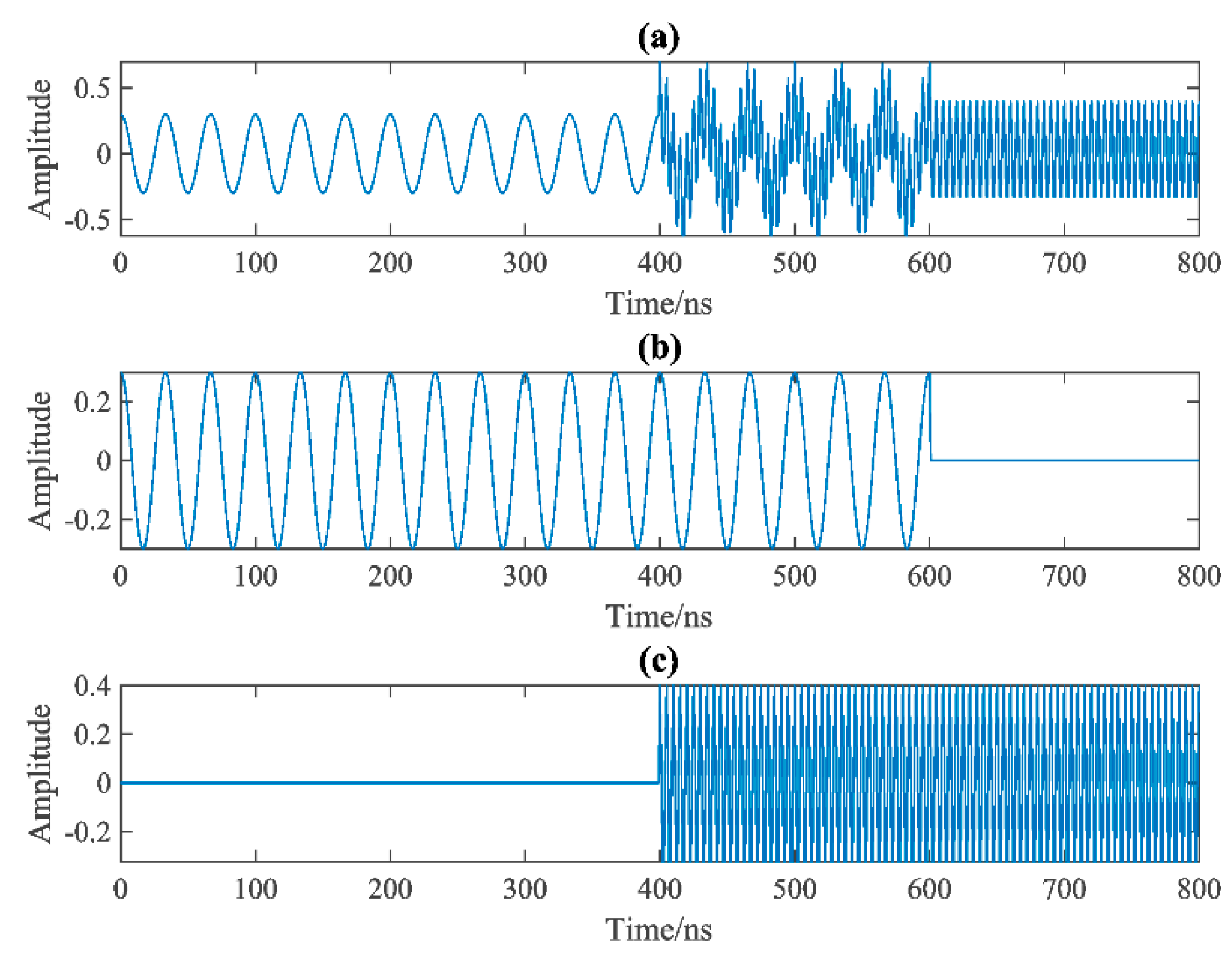
In this section, we show an example of a two−channel benchmark, where there exist three frequency modes. In the first channel (i.e., channel-1, see
Figure 1a), there are 3 MHz and 20 MHz sinusoids (see
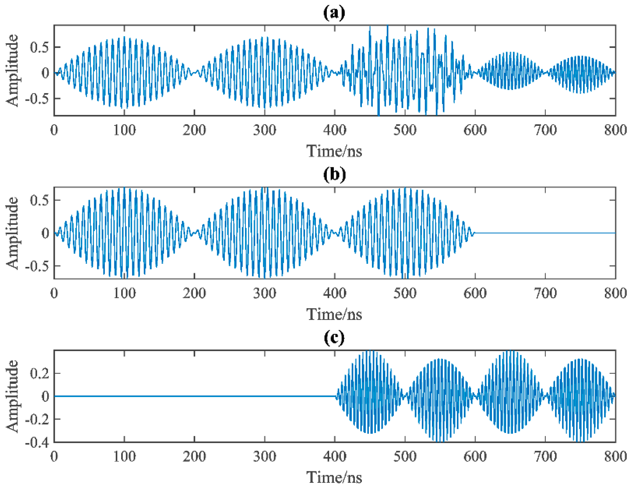
Figure 1b,c) located on both ends of the signal, while the second channel (i.e., channel-2, see
Figure 2a) consists of the 12 MHz and 20 MHz sinusoids with amplitude modulation (AM) as shown in
Figure 2b,c.
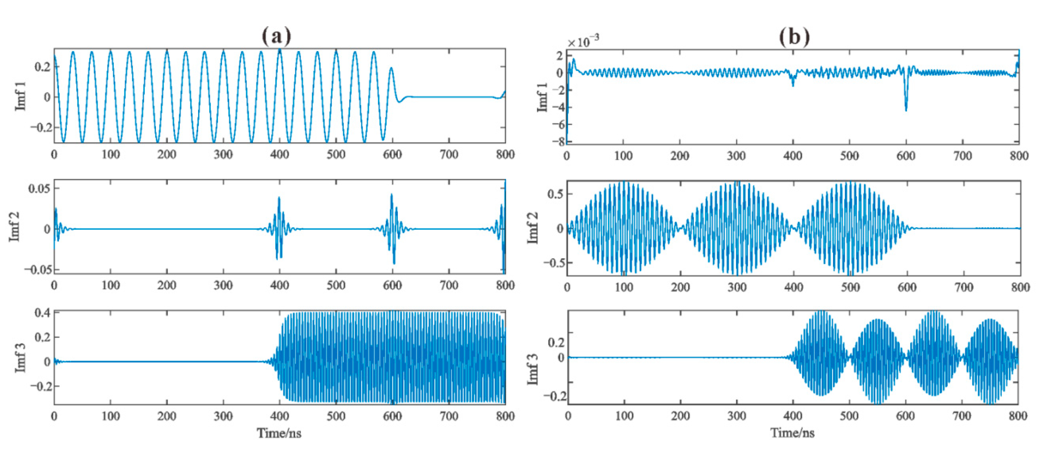
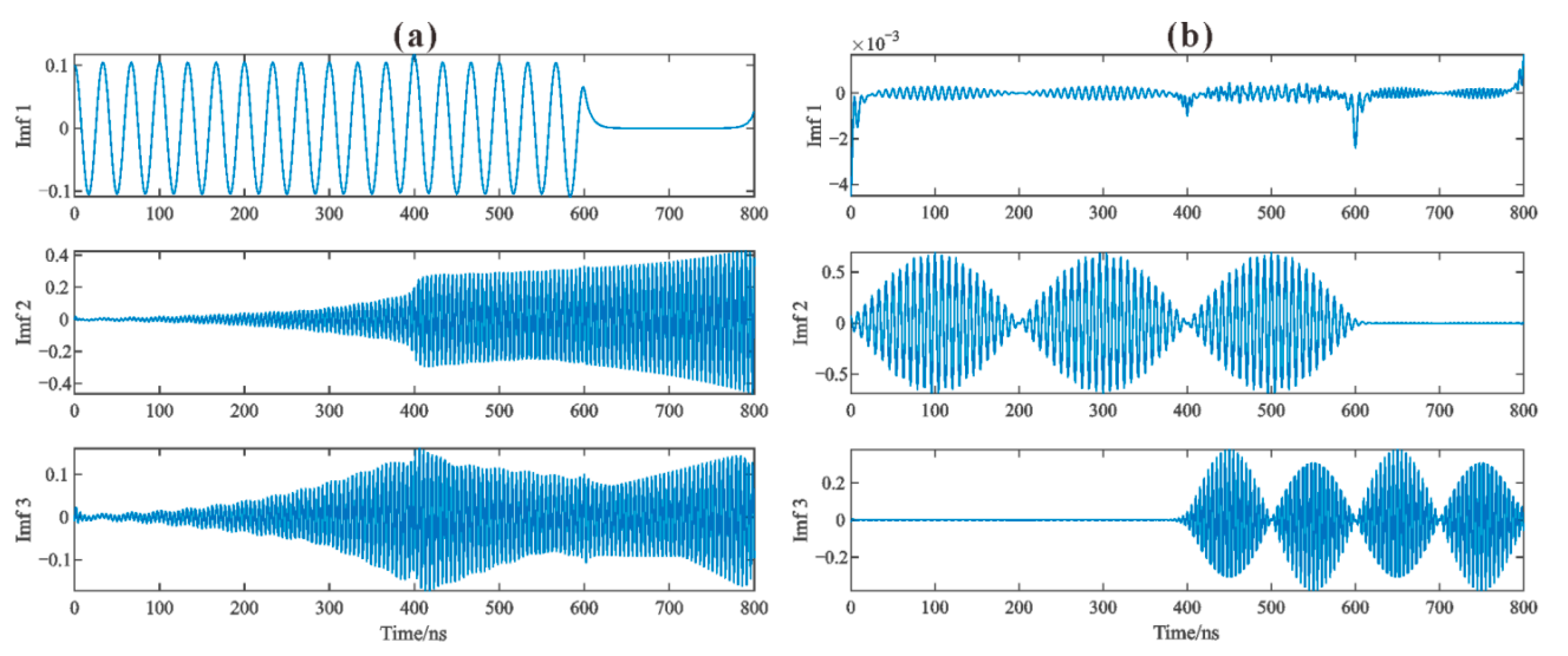
We compare the decomposition by MVMD and VMD, respectively, to demonstrate the superiority of the multi-channel decomposition scheme, as seen in
Figure 3 and
Figure 4. The values of
K in the above schemes are both set to 3. In the MVMD scheme, the two channels are taken into consideration for decomposition simultaneously, and the embedded three frequency modes are identified effectively. In channel-1 (
Figure 3a), the primary components (i.e., 3 MHz and 20 MHz) are separated into IMF1 and IMF3, while the amplitude of 12 MHz (i.e., IMF2) is small. As
Figure 3b shows, the primary frequency modes of channel-2 are mostly separated into IMF2 and IMF3, and the amplitude of 3 MHz (i.e., IMF1) is close to zero. It can be observed that there exists pattern alignment of mode frequencies in the derived IMFs between channels, which is beneficial to B-scan decomposition as well as the following construction of IMF-slices. On the contrary, in
Figure 4a, there is a severe mode−mixing phenomenon and frequency modes mismatch in the VMD decomposition due to a lack of the constraints of neighboring channels, as seen in the case of IMF2 and IMF3 for channel-1.
We further highlight the merits of MVMD from the instantaneous spectrum. Here, we use channel-1 as an example. By using the Hilbert transform technique, the instantaneous amplitude and frequency can be estimated based on the IMFs decomposed by MVMD and VMD (see
Figure 3a and
Figure 4a), and then the corresponding time-frequency representations are shown in
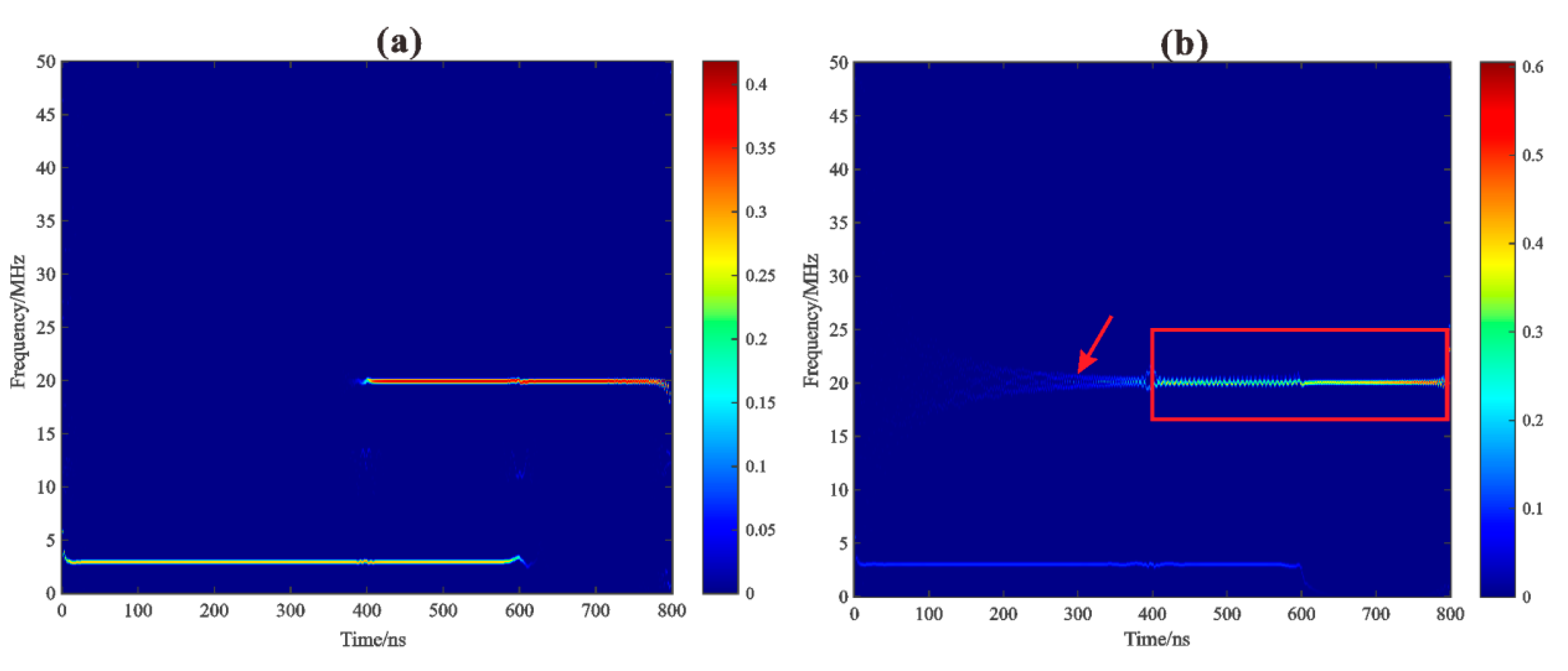
Figure 5a,b, respectively. The former tracks the 3 MHz and 20 MHz spectrum components with better resolution and convergences because the modes are well separated by the multi−channel decomposition scheme, as can be seen with the IMF1 and IMF3 in
Figure 3a. In contrast, the 20 MHz spectrum component in
Figure 5b exhibits an obvious endpoint effect (see the red arrow) and inaccurate amplitude representation (the red box).
3.2. The Forward Model Test
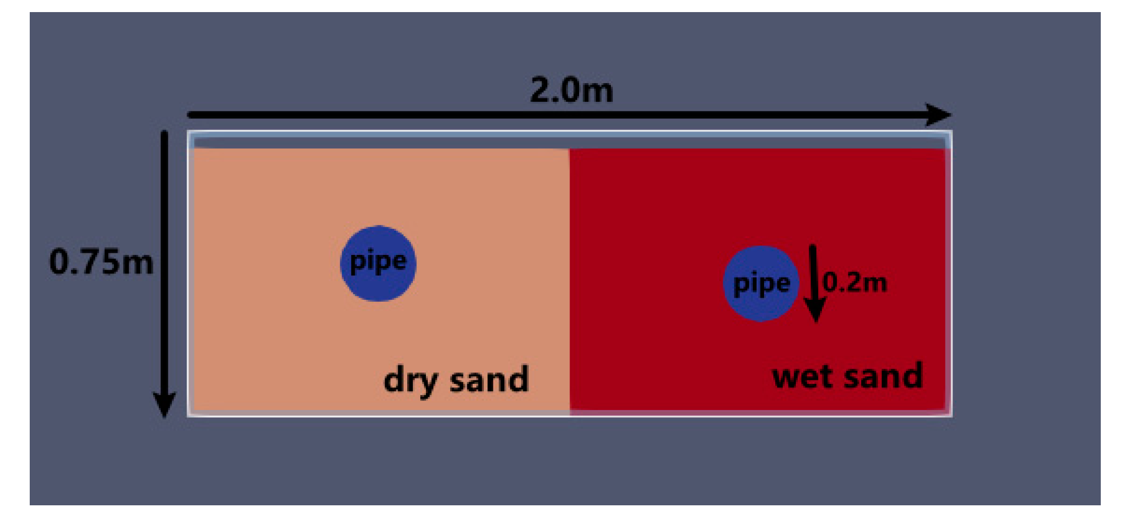
We apply the proposed method to model data by GPR forward simulation in this section. The model size is 2.0 m × 0.75 m, as in the schematic diagram shown in
Figure 6. The subsurface half−space (0.75 m−thick) consists of two parts, i.e., dry sand (
= 6,
= 0.001 S/m) and wet sand (
= 25,
= 0.005 S/m), in which two metal cylinders or pipes (
= 0.1 m) are buried, respectively. The impulse source (i.e., the transmitting antenna) with the center frequency of 900 MHz moves along the interface between the subsurface halfspace and air, and the transceiver distance is fixed as 0.4 m. The propagation of the electromagnetic wave is forward simulated using the open-sourced software GprMax3.0 [
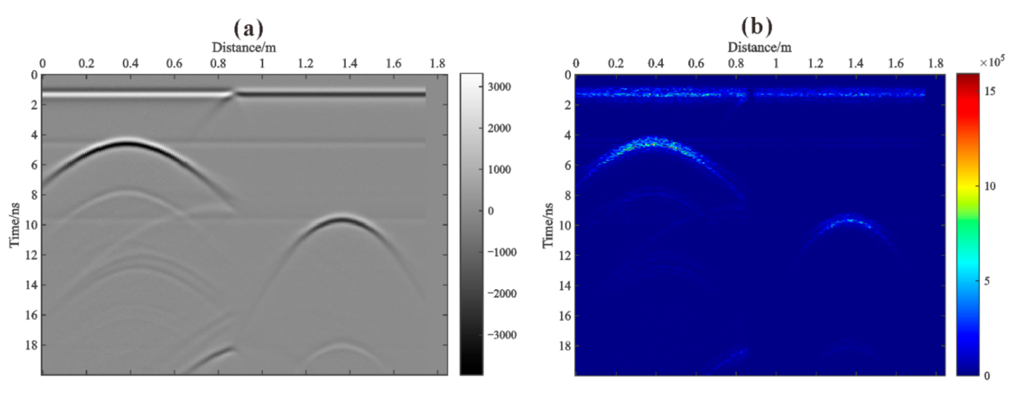
20], which is based on the finite difference in time domain (FDTD) method. The obtained GPR B−scan is shown in
Figure 7a, which contains 180 A-scans and 1024 samples. We added Gaussian random noise (SNR = 20). It can be observed that the first-arrivals and the reflections by the two metal pipes are more obvious than the multiples in the deep part.
The operator of TKEO is only valid for describing the energy attributes of mono-component or narrow-bandwidth signals [
16]. The waveform of each A−scan and the frequency components fluctuate due to the earth filtering and the noise interference. This phenomenon is referred to as the “non−stationarity” of geophysical data, which may affect the tracking of the reflection energy of the TKEO. When we perform the TKEO on each A−scan in
Figure 7a directly, the resolution of the derived TKEO profile (see
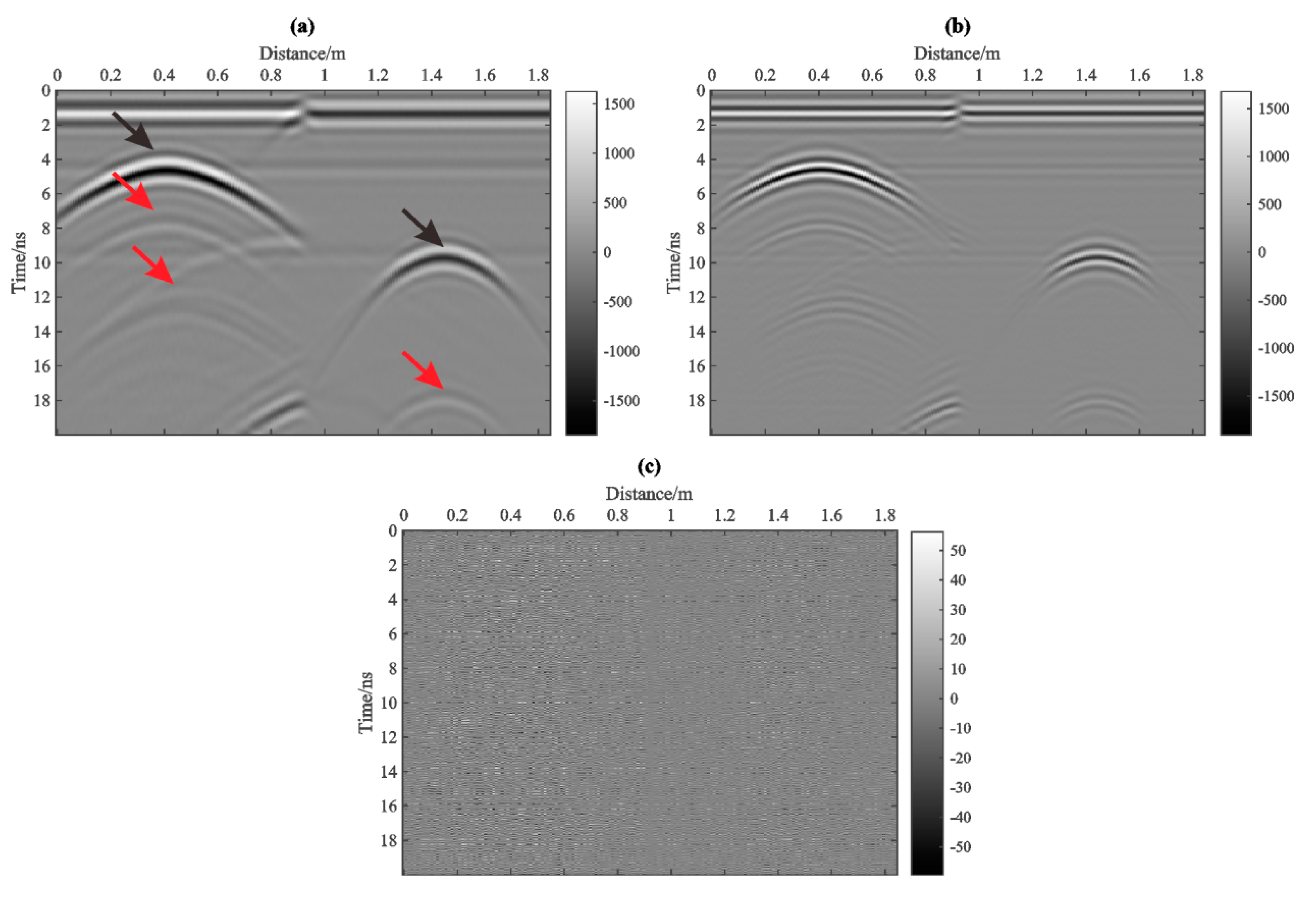
Figure 7b) is poor. In order to meet the applicable condition of the TKEO, we obtain the IMF-slices corresponding to three different frequency ranges (
K = 3, see
Figure 8) by using the MVMD.
Figure 8a,b are the IMF-slices corresponding to the low- and medium-frequency vibration modes, where the direct wave and the first-arrivals by metal pipes can be seen, as indicated by the black arrows. There are several multiples at the bottom (see the red arrows), which affects target identification.
Figure 8c show the high−frequency IMF-slice, which contain little meaningful information aside from the noise.
In
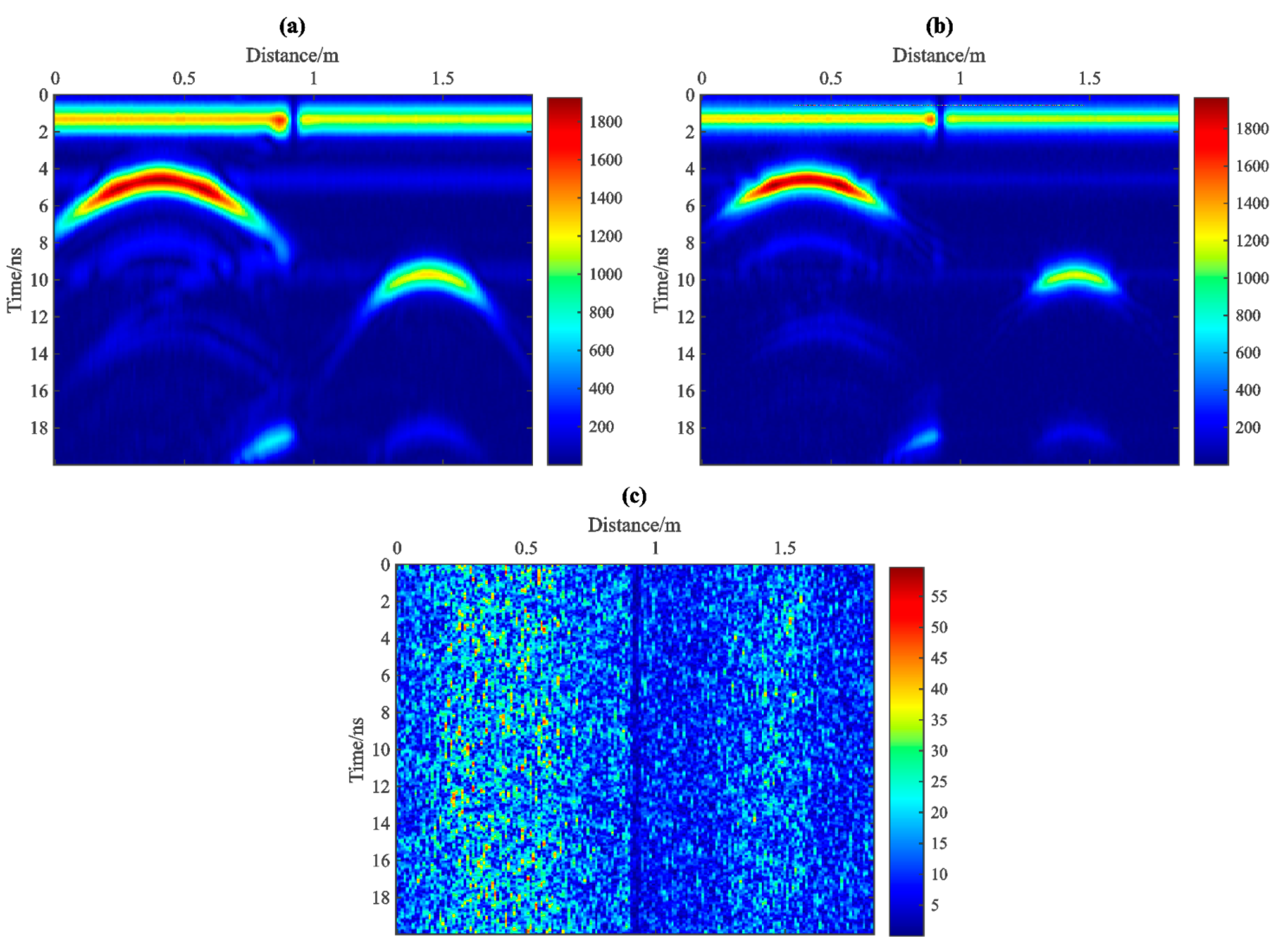
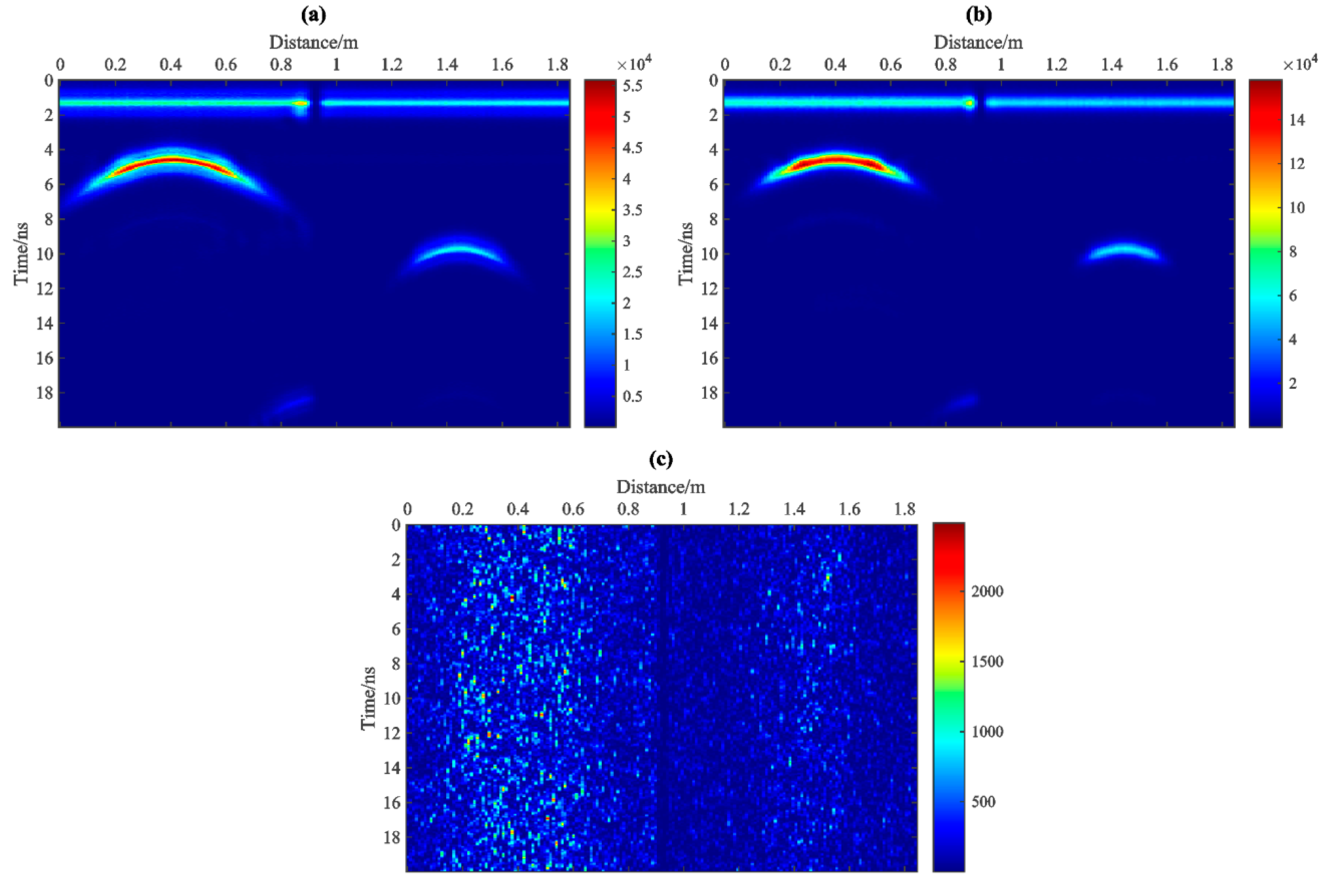
Figure 9, we extract the instantaneous energy attributes of the above IMF-slices derived by the MVMD. Although the energy components of all the target bodies can be observed, the time−frequency resolution is low. We then perform the TKEO on A−scans within each IMF-slice, and the derived TKEO-slices are shown in
Figure 10. The first two TKEO-slices are shown in
Figure 10a,b, and the reflections for the metal pipes are displayed more distinctly, while the multiples at the deep part disappear. The above results prove the superior effectiveness of the TKEO in gathering energy and suppressing multiple reflections.
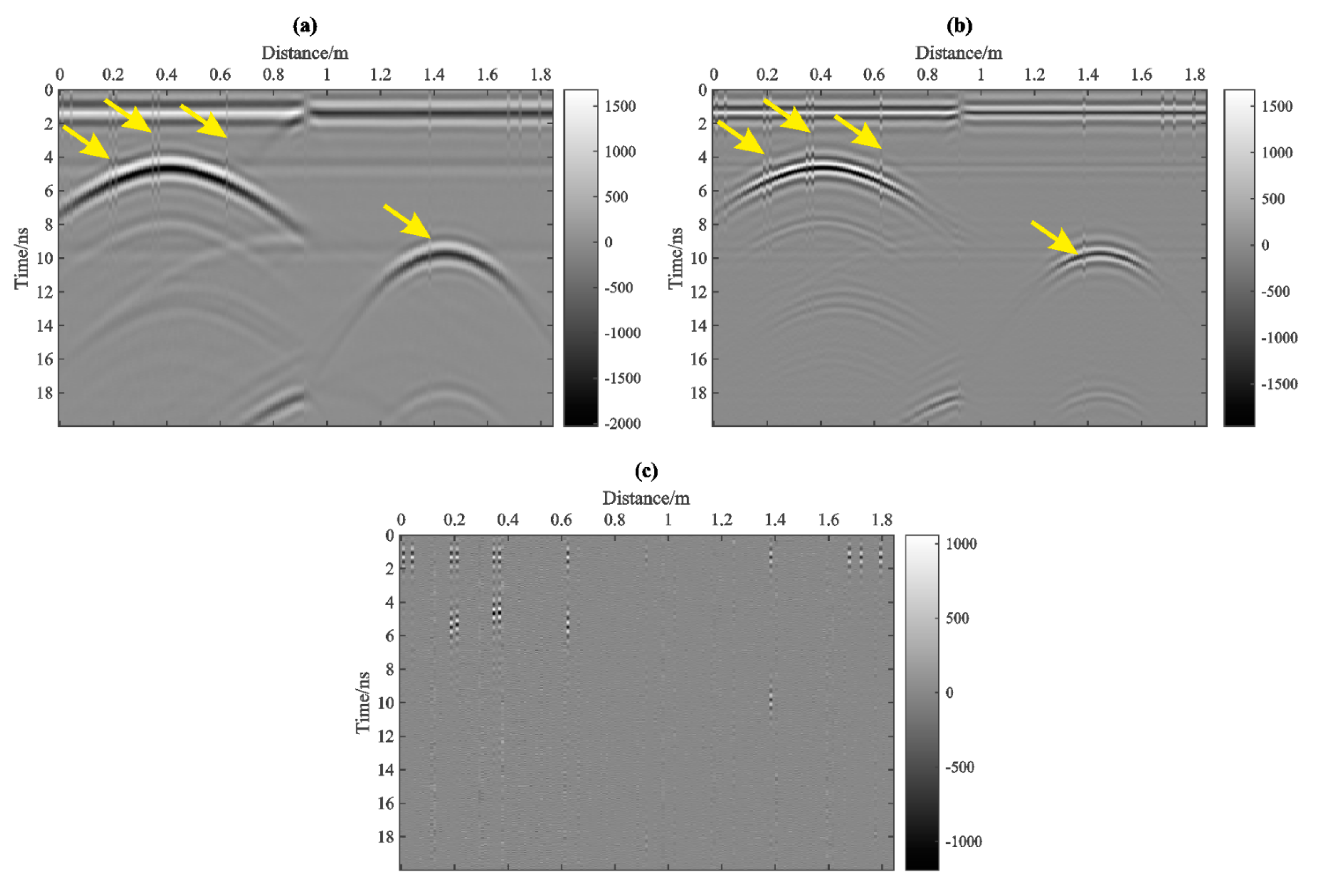
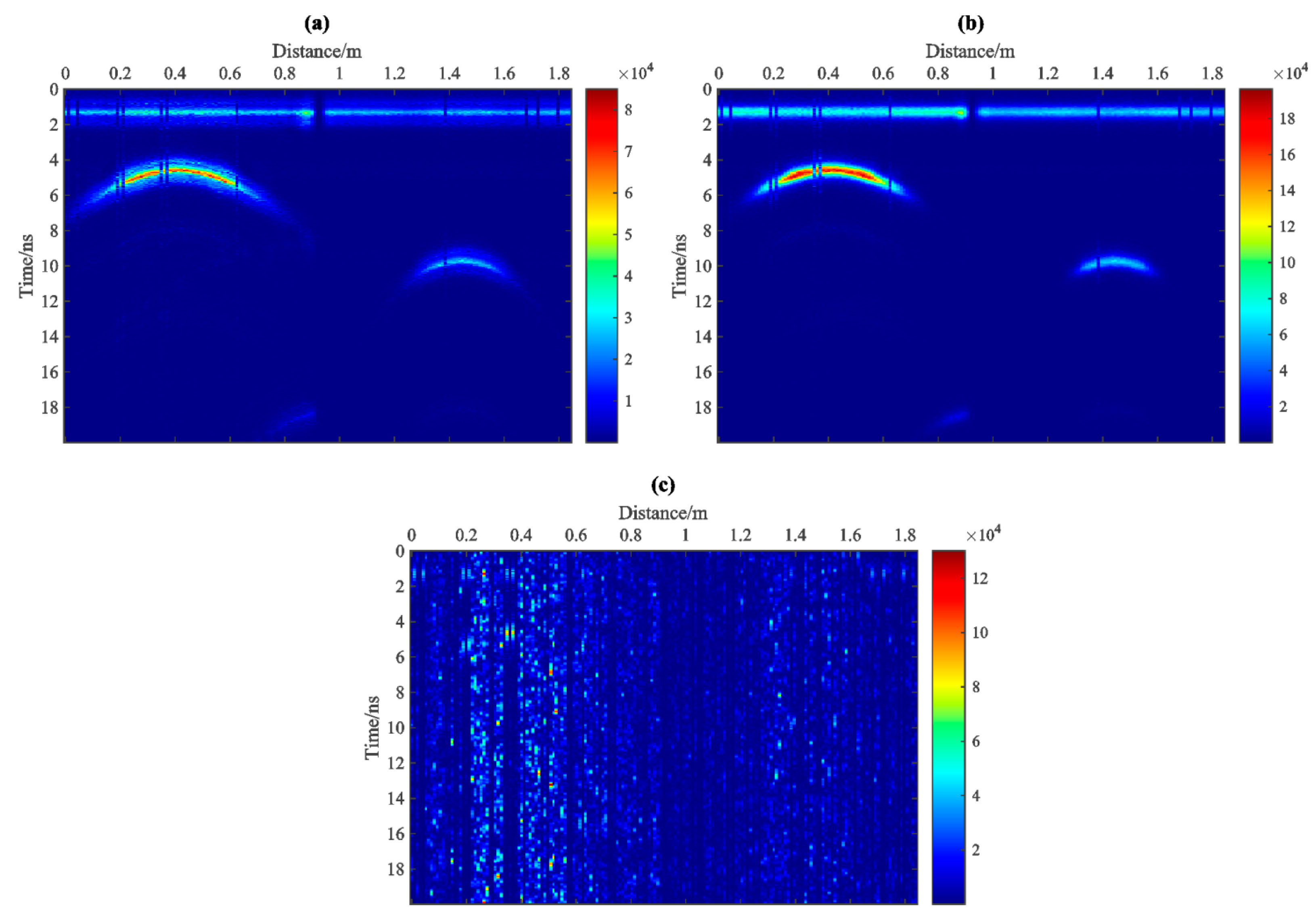
As a comparison, we decompose the model data using VMD trace-by-trace, and the following processing is the same as the MVMD−based method. From
Figure 11, we observe that the IMF-slices obtained by using VMD are less effective than MVMD, e.g., the discontinuity at adjacent traces appears in the positions indicated by the yellow arrows. The lateral discontinuity is more visible from the corresponding TKEO-slices, as seen in
Figure 12, because the trace-by-trace decomposition of VMD may cause the similar frequency modes in the IMF-slices to be misaligned.
The above discussion verifies that the MVMD−based TKEO slicing has better resolution for identifying subsurface target bodies than the VMD−based method, because it avoids the frequency modes being misaligned and the discontinuity of adjacent channels.
3.3. Field Data
In this section, a GPR field data is applied here to further evaluate the proposed method. The field data is acquired using the Mala GPR system and 800 MHz antenna on a transversal section of the silt region in France. The measurement length is 5.09 m, and the acquisition details can be referred to in Chapter 3.3.1 of the project instructions of the TU1208 Open Database [
21].
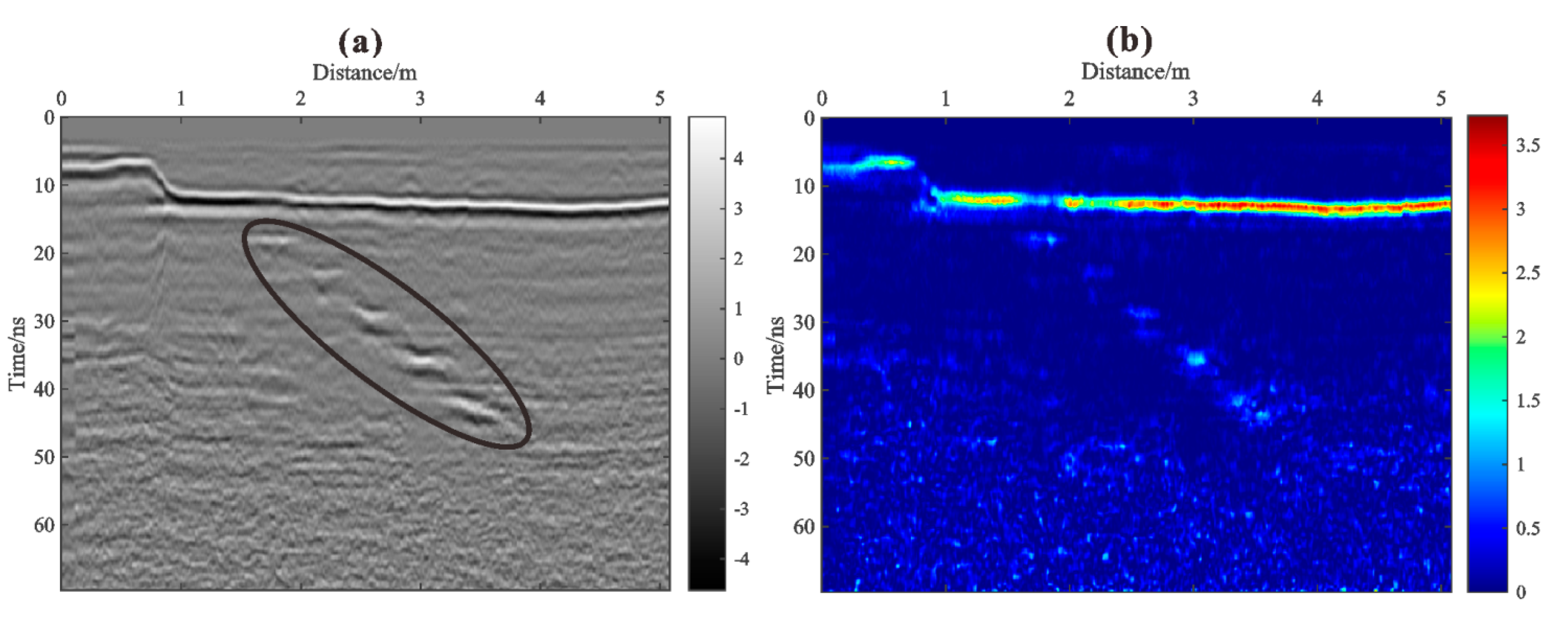
Figure 13a shows the B−scan of the field data, where five voids are indicated by the black circle.
As mentioned in the previous sections, the direct TKEO calculation on raw GPR data does not meet the application condition, and the corresponding TKEO profile cannot illustrate the subsurface voids due to the low resolution, as seen in
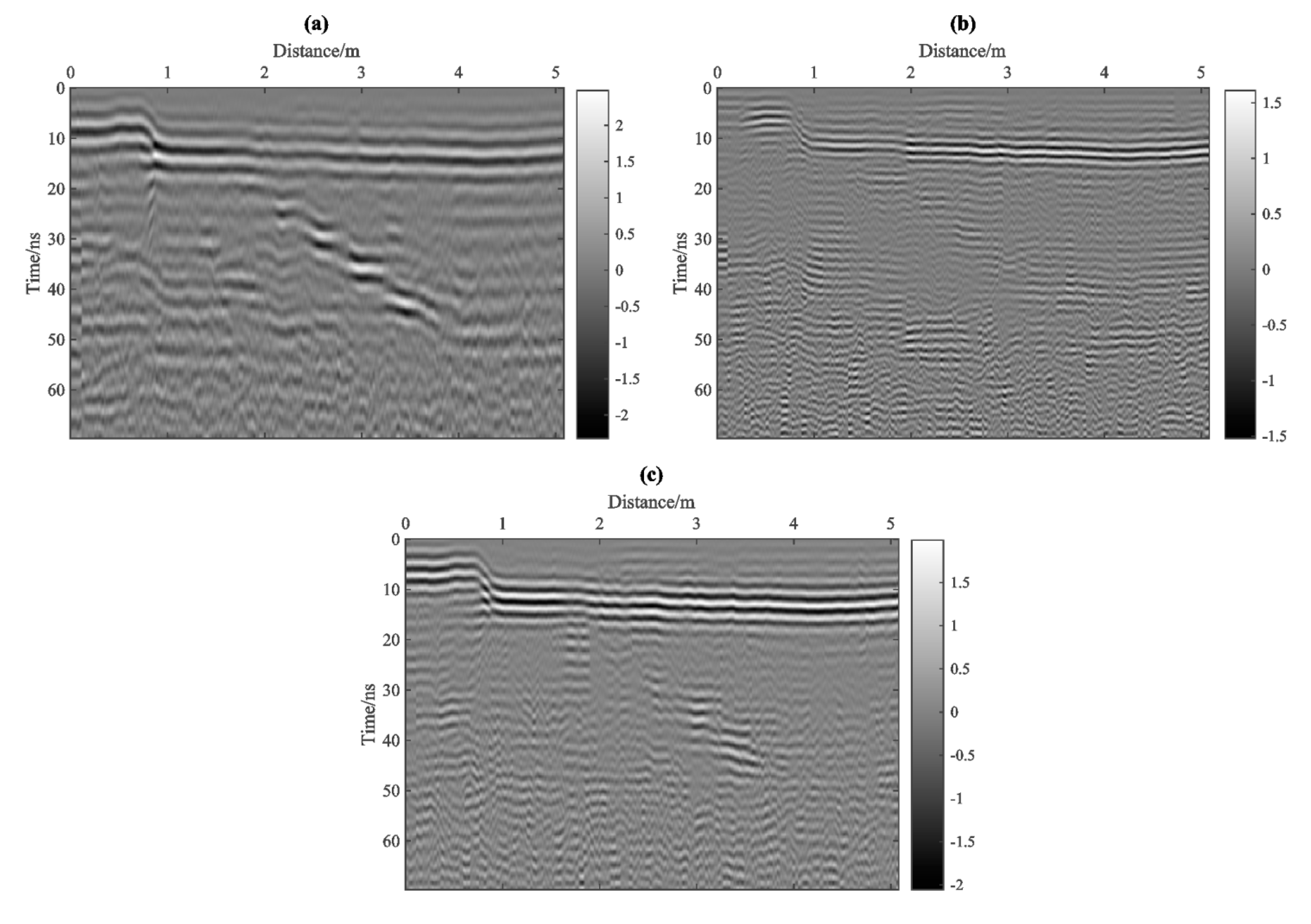
Figure 13b. By using the MVMD, the A-scans of the field data are decomposed simultaneously to obtain three IMF-slices, which show different scales of geophysical information with good stratigraphic continuity, as seen in
Figure 14.
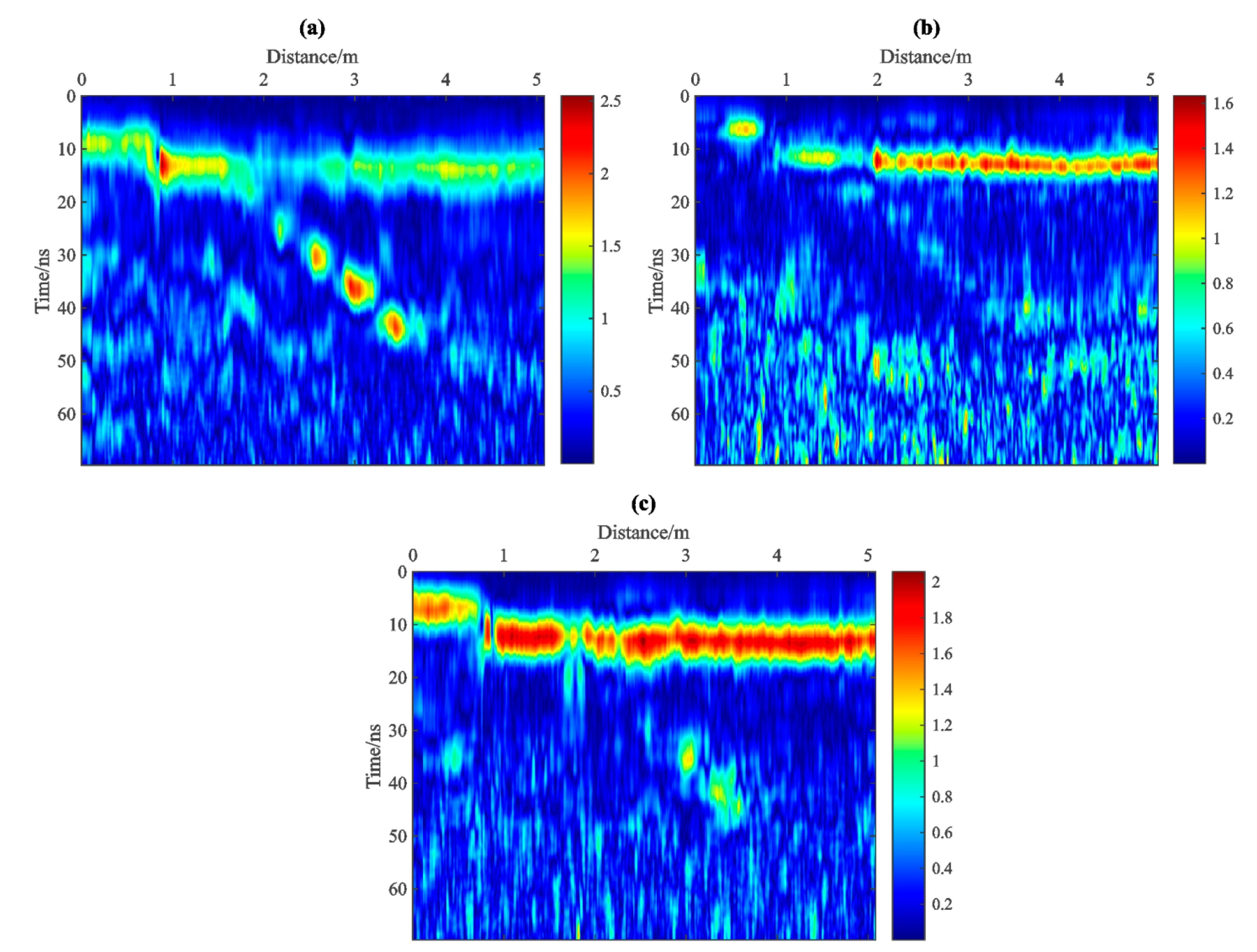
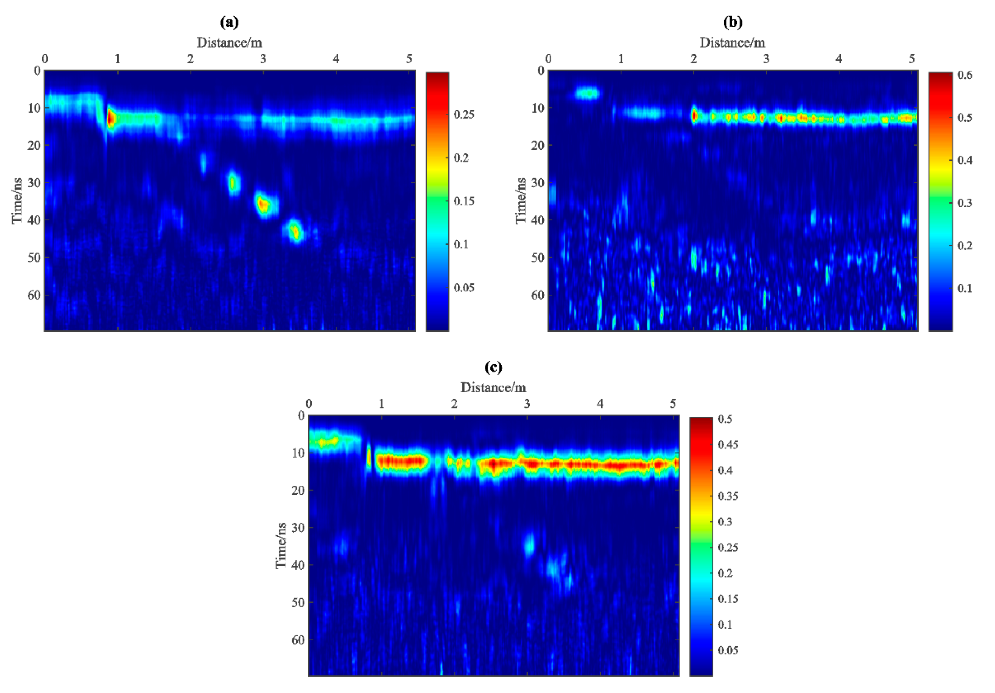
Based on the above IMF-slices, we derive the corresponding instantaneous amplitude profiles and TKEO-slices, as seen in
Figure 15 and
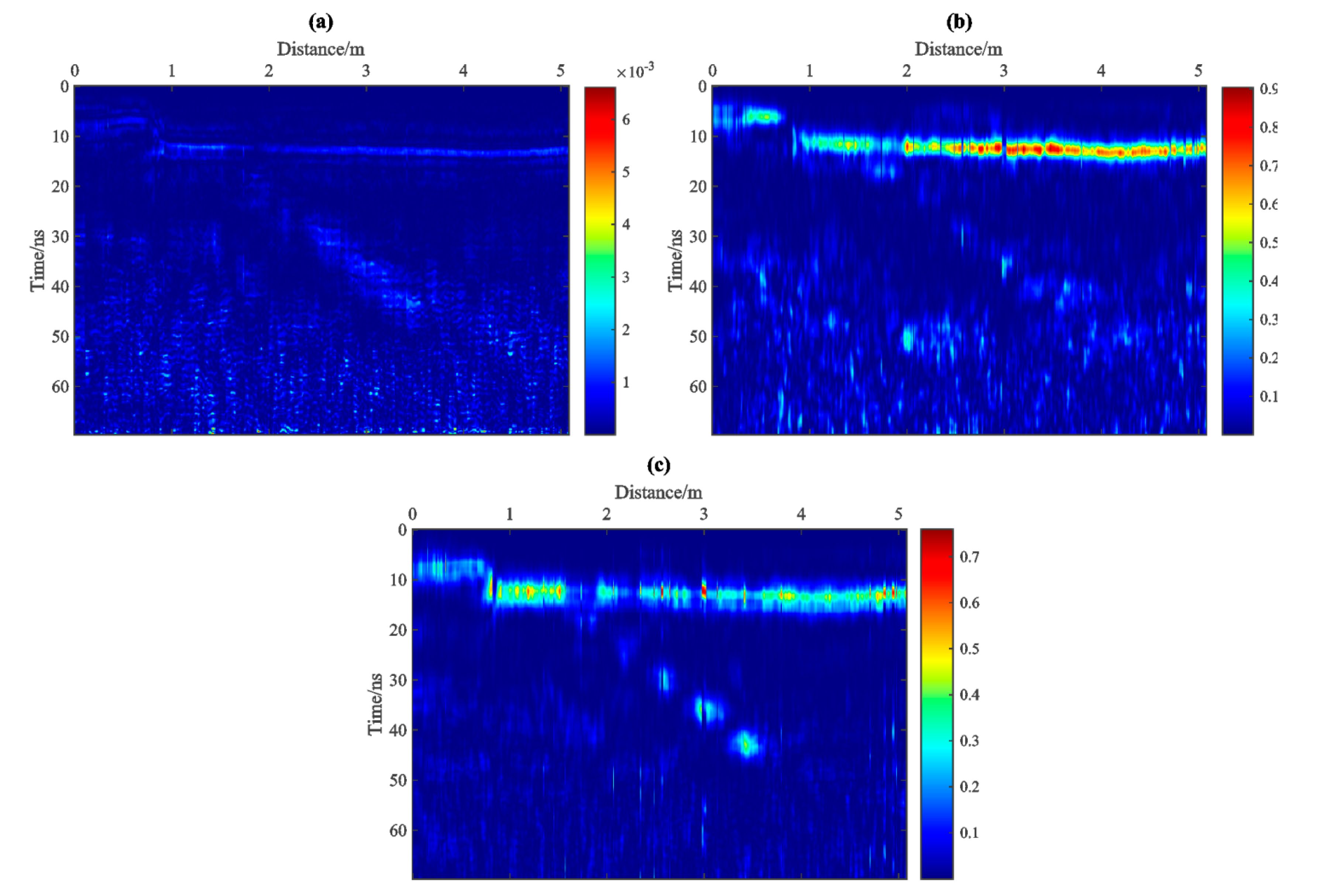
Figure 16, where the phenomenon of the “low-frequency anomalies” can be observed. Specifically, the low-frequency TKEO-slice (i.e.,
Figure 16a) highlights the horizontal layers and voids and, in the medium- and high-frequency TKEO-slices, the energy for the voids gradually decays until it becomes very weak, as seen in
Figure 16b,c.
Figure 15a–c are the classical instantaneous amplitude attributes for the IMF-slices showing the similar features in lower resolution. It is obvious that the TKEO-slices are less disturbed by the noise and multiple reflections at the deep part of the profiles, which show better performance in gathering the energy at the location of voids.
For comparative analysis, we apply the VMD to each A−scan of the field data, and then collect the IMFs of same order into three IMF-slices (
K = 3), as seen in
Figure 17. The drawback of the trace−by−trace decomposition scheme is obvious, e.g., the discontinuity between adjacent traces due to misaligned frequency modes, marked by the red arrows between 3~4 m. The results of the TKEO computation based on the VMD−based IMF-slices are shown in
Figure 18, where the resolution and lateral continuity is affected by the incomplete decomposition of VMD. The above application on the field data shows that the proposed method has an obvious response to the anomaly targets in the subsurface medium, and proves the effectiveness of the TKEO in gathering energy and suppressing multiple reflections.
4. Discussion
The GPR profiles can be decomposed by the EMD−like decompositions into several IMFs, and the derived IMFs have found many applications in geophysical data processing. The VMD decomposition eliminates the drawback of EMD (e.g., mode mixing and endpoint effects) to some extent, but the decomposition is still executed in one dimension. In this work, we introduce the MVMD scheme to decompose the GPR B-scan data in two dimensions, which inherits the advantages of the VMD scheme and considers the stratigraphic constraints. We have shown three application examples of the proposed energy attribute slices for GPR data based on the MVMD and TKEO. From the synthetic benchmark, it can be observed that the IMFs derived in the MVMD decomposition are less subject to the “mode-mixing” phenomenon by using the merit of the constraints of neighboring A-scans. From the GPR IMF-slices shown in Part 3, we find that the extracted IMF-slices using the multi−channel decomposition scheme show better stratigraphic continuity. Based on the above merits, the TKEO can be effectively performed on each IMF-slice to localize the energy attributes (i.e., the TKEO-slices), and the subsurface target bodies and geological structures can be interpreted in high resolution. The application examples prove the superiority of the proposed method in GPR data processing, compared with the VMD-based scheme and the classic instantaneous amplitude.
Furthermore, we noticed that the proposed TKEO-slices are somewhat similar to the “common-frequency slices” in seismic processing. The common-frequency slices only reveal the energy attributes at certain frequencies, while the proposed TKEO-slices provide the corresponding results at different frequency ranges more flexibly. Because the operator of TKEO only performs well on the quasi−harmonic or mono-component frequency modes, the performance of the proposed TKEO-slices depends on the results of mode decomposition. However, as with VMD, the parameters in the MVMD decomposition (e.g., the number of decomposition K and penalty factor α) still need to be selected artificially, which may affect the decomposition effect of the MVMD, as well as the resolution of the proposed TKEO-slices. In future work, we will work on estimating the parameters in the optimization to improve the decomposition results and provide scientific methods to evaluate the validity, so that the proposed TKEO-slices can be better applied to GPR data. In addition, the ADMM is applied to solve the constrained optimization in MVMD, which takes a lot of computational time, so we will try to apply other more effective optimization algorithms to solve this issue.
5. Conclusions
In this paper, we propose a novel workflow for GPR data processing, which can localize the energy attributes and identify subsurface target bodies or geological structures effectively. The MVMD is introduced to decompose the GPR B-scan into a series of band−limited IMF-slices, which can enhance the lateral continuity of the IMFs and feature the geological events of the subsurface medium in multiple directions. Based on the above merits, the TKEO is then performed on each IMF-slice to localize the energy attributes (i.e., the TKEO-slices), and the subsurface target bodies and geological structures can be interpreted in higher resolution. We have shown three application examples of the proposed energy attribute slices for GPR data based on the MVMD and TKEO, which show the superiority of the proposed method in GPR data processing, compared with the VMD−based scheme and the classic instantaneous amplitude.
Author Contributions
X.Z. and X.F. managed the project; X.Z., Y.Q. and Y.C. conceived and designed the experiments; Z.H.; performed the experiments; X.Z., Y.Q. and X.H. analyzed the data, wrote the code and made the visualization; X.Z. and Y.Q. wrote the paper and made the revision. All authors have read and agreed to the published version of the manuscript.
Funding
This work is supported in part by the National Natural Science Foundation of China under Grant 42004129, the National Key Research and Development Program of China under Grant 2021YFC1523401 and the Education Department of Jilin Province (JJKH20210251KJ, JJKH20190879KJ).
Data Availability Statement
Acknowledgments
The authors thank the three anonymous reviewers for the meaningful and inspiring discussions.
Conflicts of Interest
The authors declare no conflict of interest.
References
- Stockwell, R.G.; Mansinha, L.; Lowe, R.P. Localization of the complex spectrum: The S transform. IEEE Trans. Signal Process. 1996, 44, 998–1001. [Google Scholar] [CrossRef]
- Cheng, Z.; Chen, W.; Chen, Y.; Liu, Y.; Liu, W.; Li, H.; Yang, R. Application of bi-Gaussian S-transform in high-resolution seismic time-frequency analysis. Interpretation 2017, 5, SC1–SC7. [Google Scholar] [CrossRef]
- Rioul, O.; Vetterli, M. Wavelets and signal processing. IEEE Signal Process. Mag. 1991, 8, 14–38. [Google Scholar] [CrossRef]
- Sinha, S.; Routh, P.S.; Anno, P.D.; Castagna, J.P. Spectral decomposition of seismic data with continuous-wavelet transform. Geophysics 2005, 70, P19–P25. [Google Scholar] [CrossRef]
- Huang, N.E.; Wu, Z.; Long, S.R.; Arnold, K.C.; Chen, X.; Blank, K. On instantaneous frequency. Appl. Comput. Harmon. Anal. 2009, 1, 177–229. [Google Scholar] [CrossRef]
- Huang, N.E.; Shen, Z.; Long, S.R.; Wu, M.C.; Shih, H.H.; Zheng, Q.; Yen, N.C.; Tung, C.C.; Liu, H.H. The empirical mode decomposition and the Hilbert spectrum for nonlinear and non-stationary time series analysis. Proc. R. Soc. A 1998, 454, 903–995. [Google Scholar] [CrossRef]
- Wu, Z.; Huang, N.E. Ensemble empirical mode decomposition: A noise-assisted data analysis method. Adv. Adapt. Data Anal. 2011, 1, 1–41. [Google Scholar] [CrossRef]
- Torres, M.E.; Colominas, M.A.; Schlotthauer, G.; Flandrin, P. A complete ensemble empirical mode decomposition with adaptive noise. In Proceedings of the 2011 IEEE International Conference on Acoustics, Speech and Signal Processing (ICASSP), Prague, Czech Republic, 22–27 May 2011; pp. 4144–4147. [Google Scholar]
- Li, J.; Liu, C.; Zeng, Z.; Chen, L. GPR Signal Denoising and Target Extraction with the CEEMD Method. IEEE Geosci. Remote Sens. Lett. 2015, 12, 1615–1619. [Google Scholar]
- Dragomiretskiy, K.; Zosso, D. Variational Mode Decomposition. IEEE Trans. Signal Process. 2014, 62, 531–544. [Google Scholar] [CrossRef]
- Liu, W.; Cao, S.; Chen, Y. Applications of variational mode decomposition in seismic time-frequency analysis. Geophysics 2016, 81, V365–V378. [Google Scholar] [CrossRef]
- Ur Rehman, N.; Aftab, H. Multivariate Variational Mode Decomposition. IEEE Trans. Signal Process. 2019, 67, 6039–6052. [Google Scholar] [CrossRef]
- Liu, N.; Li, F.; Wang, D.; Gao, J.; Xu, Z. Ground-Roll Separation and Attenuation Using Curvelet-Based Multichannel Variational Mode Decomposition. IEEE Trans. Geosci. Remote Sens. 2022, 60, 5901214. [Google Scholar] [CrossRef]
- Zhang, X.; Nilot, E.; Feng, X.; Ren, Q.; Zhang, Z. IMF-Slices for GPR Data Processing Using Variational Mode Decomposition Method. Remote Sens. 2018, 10, 476. [Google Scholar] [CrossRef]
- Teager, H.M.; Teager, S.M. Evidence for nonlinear sound production mechanisms in the vocal tract. Speech Prod. Speech Model. 1990, 55, 241–261. [Google Scholar]
- Kaiser, J.F. On a simple algorithm to calculate the ‘energy’ of a signal. In Proceedings of the International Conference on Acoustics, Speech, and Signal Processing, Albuquerque, NM, USA, 3–6 April 1990; pp. 381–384. [Google Scholar]
- Liu, W.; Cao, S.; Wang, Z.; Kong, X.; Chen, Y. Spectral Decomposition for Hydrocarbon Detection Based on VMD and Teager–Kaiser Energy. IEEE Geosci. Remote Sens. Lett. 2017, 14, 539–543. [Google Scholar] [CrossRef]
- Xue, Y.J.; Cao, J.X.; Tian, R.F. EMD and Teager–Kaiser energy applied to hydrocarbon detection in a carbonate reservoir. Geophys. J. Int. 2014, 197, 277–291. [Google Scholar] [CrossRef]
- Boyd, S.; Parikh, N.; Chu, E.; Peleato, B.; Eckstein, J. Distributed Optimization and Statistical Learning via the Alternating Direction Method of Multipliers. Found. Trends Mach. Learn. 2011, 3, 1–122. [Google Scholar] [CrossRef]
- Giannopoulos, A. Modelling ground penetrating radar by GprMax. Constr. Build. Mater. 2005, 19, 755–762. [Google Scholar] [CrossRef]
- Dérobert, X.; Pajewski, L. TU1208 Open Database of Radargrams: The Dataset of the IFSTTAR Geophysical Test Site. Remote Sens. 2018, 10, 530. [Google Scholar] [CrossRef]
Figure 1.
The first channel of the synthetic benchmark (channel-1) (a) composed of two sub-components (b,c).
Figure 1.
The first channel of the synthetic benchmark (channel-1) (a) composed of two sub-components (b,c).
Figure 2.
The second channel of the synthetic benchmark (channel-2) (a) composed of two sub-components (b,c).
Figure 2.
The second channel of the synthetic benchmark (channel-2) (a) composed of two sub-components (b,c).
Figure 3.
The MVMD decomposition results for (a) the simulated channel-1 and (b) channel-2.
Figure 3.
The MVMD decomposition results for (a) the simulated channel-1 and (b) channel-2.
Figure 4.
The VMD decomposition results for (a) the simulated channel-1 and (b) channel-2.
Figure 4.
The VMD decomposition results for (a) the simulated channel-1 and (b) channel-2.
Figure 5.
Time−frequency representation of channel−1 based on (a) the MVMD and (b) the VMD, respectively.
Figure 5.
Time−frequency representation of channel−1 based on (a) the MVMD and (b) the VMD, respectively.
Figure 6.
Schematic diagram of the forward model for GPR FDTD simulation.
Figure 6.
Schematic diagram of the forward model for GPR FDTD simulation.
Figure 7.
(a) GPR B-scan based on the forward model and (b) the derived profile by directly performing the TKEO.
Figure 7.
(a) GPR B-scan based on the forward model and (b) the derived profile by directly performing the TKEO.
Figure 8.
IMF-slices of the GPR simulation model using MVMD. (a−c) show the IMF-slices 1−3, respectively.
Figure 8.
IMF-slices of the GPR simulation model using MVMD. (a−c) show the IMF-slices 1−3, respectively.
Figure 9.
(a−c) show the instantaneous amplitude profiles of IMF-slices 1−3 for the GPR forward model using MVMD, respectively.
Figure 9.
(a−c) show the instantaneous amplitude profiles of IMF-slices 1−3 for the GPR forward model using MVMD, respectively.
Figure 10.
TKEO-slices of the model data using MVMD. (a−c) show the TKEO-slices 1−3, respectively.
Figure 10.
TKEO-slices of the model data using MVMD. (a−c) show the TKEO-slices 1−3, respectively.
Figure 11.
IMF-slices of the model data using VMD. (a−c) show the IMF-slices 1−3, respectively.
Figure 11.
IMF-slices of the model data using VMD. (a−c) show the IMF-slices 1−3, respectively.
Figure 12.
TKEO-slices of the model data using VMD. (a−c) show the TKEO-slices 1−3, respectively.
Figure 12.
TKEO-slices of the model data using VMD. (a−c) show the TKEO-slices 1−3, respectively.
Figure 13.
(a) B-scan of the field data, where the black circle indicates the voids; (b) the profile produced by performing the TKEO directly.
Figure 13.
(a) B-scan of the field data, where the black circle indicates the voids; (b) the profile produced by performing the TKEO directly.
Figure 14.
IMF-slices of the field data using MVMD. (a−c) show the IMF-slices 1−3, respectively.
Figure 14.
IMF-slices of the field data using MVMD. (a−c) show the IMF-slices 1−3, respectively.
Figure 15.
The instantaneous amplitude profiles of IMF-slices 1−3 (a−c) for the field data by using MVMD, respectively.
Figure 15.
The instantaneous amplitude profiles of IMF-slices 1−3 (a−c) for the field data by using MVMD, respectively.
Figure 16.
The MVMD-based TKEO-slices of the field data. (a−c) show the TKEO-slices 1−3, respectively.
Figure 16.
The MVMD-based TKEO-slices of the field data. (a−c) show the TKEO-slices 1−3, respectively.
Figure 17.
IMF-slices of the field data using VMD. (a−c) show the IMF-slices 1−3, respectively.
Figure 17.
IMF-slices of the field data using VMD. (a−c) show the IMF-slices 1−3, respectively.
Figure 18.
TKEO-slices of the field by using VMD. (a−c) show the TKEO-slices 1−3, respectively.
Figure 18.
TKEO-slices of the field by using VMD. (a−c) show the TKEO-slices 1−3, respectively.
| Publisher’s Note: MDPI stays neutral with regard to jurisdictional claims in published maps and institutional affiliations. |
© 2022 by the authors. Licensee MDPI, Basel, Switzerland. This article is an open access article distributed under the terms and conditions of the Creative Commons Attribution (CC BY) license (https://creativecommons.org/licenses/by/4.0/).
