Anti-Jamming Method and Implementation for GNSS Receiver Based on Array Antenna Rotation

Abstract

Global navigation satellite system (GNSS) array antenna receivers are effective for suppressing wideband jamming. However, its anti-jamming performance decreases sharply when the number of wideband interference surpasses the number of array elements. Since a large number of jammers are often used in navigation countermeasures, it is crucial to keep array antenna receivers available in such conditions. Aiming at this issue, two main tasks were performed in this research and are presented in this paper: Firstly, the direction sensitivity of the sup-freedom anti-jamming performance is revealed and an anti-jamming method for array antenna receivers based on antenna rotation is proposed. Secondly, in order to determine the optimal rotation angle rapidly, a variable-step iteration algorithm based on gradient descent is proposed. Theoretical analysis and simulation show the effectiveness of the proposed anti-jamming method and the efficiency of the implementation algorithm. In a typical airborne scenario with a maximum azimuth difference of 90°, the anti-jamming ability of the proposed method improved by 21~26 dB and 5~10 dB for arrays adopting the PI (power inversion) and MVDR (minimum variance distortionless response) algorithms, respectively. The iterative efficiency improved by 78.35–99.63% in comparison with a traversal of 0.1° search resolution. The proposed method and algorithm are not limited to airborne scenarios and they might be influential to anti-jamming algorithms in the data domain.

1. Introduction

A global navigation satellite system (GNSS) provides convenient position navigation and timing services for its application terminals [1]. It has played a fundamental role in transportation, marine fisheries, geo-hazards monitoring, emergency rescue, etc. However, the power of received GNSS signals on the ground is weak [2], which is 30 dB lower than the thermal noise of receivers [3]. The intentional interference (indicating jamming in this paper) usually leads to the decrease of the carrier-to-noise ratio (CNR), which further causes the failure of GNSS signal acquisition and tracking [4] and disables the receiver.

In navigation countermeasures, distributed wideband interference is often used [5], especially when the number of jammers is equal to or larger than the number of array elements. This is denoted as “sup-freedom interference” on the premise that the interference steering vectors are not linearly correlated to each other [6].

Sup-freedom interference is fatal to GNSS array antenna receivers. On the one hand, it is hard to suppress it completely by utilizing the orthogonality between spatial filter coefficients and interference steering vectors [7,8]. On the other hand, most GNSS array antennas only have 4~7 elements [9,10]. It is easier to increase the amount of interference than to increase the number of array elements due to limited space for navigation facilities, the half-wavelength of the L-band GNSS signal, and the lower cost of jamming equipment [11].

There is some literature on the wideband sup-freedom interference suppression technology of array antennas. In some fields, some research on antenna freedom is increasing, including studies of sparse array [12], virtual antenna array [13], polarizing array antenna [14], and synthetic aperture antennas [15]. They might be helpful against sup-freedom jamming, but they also have limitations, such as receiver dynamic, real-time computing burden, and hardware complicity [16,17]. Instead of increasing antenna freedom, the current researchers tried to improve the anti-jamming performance from a different aspect: by utilizing the direction sensitivity of spatial anti-jamming performance.

The contents of the paper are as follows: Section 2 establishes the array signal reception and anti-jamming model. Section 3 analyzes the direction-sensitivity of sup-freedom anti-jamming performance and proposes an antenna rotation method against sup-freedom interference. Section 4 proposes a variable-step iteration algorithm based on gradient descent in order to efficiently obtain the optimal rotation angle. Section 5 presents simulations and analysis. Section 6 discusses the future work. The major contributions are included in Section 3 and Section 4. A block diagram of the article structure is shown in Figure 1.

In order to make it easier for reading, frequently used symbols are listed in

Table 1. Frequently used symbols.

Symbol	Explanation
${[\cdot ]}^{\mathrm{H}}$	“H” means Hermitian Transpose
${[\cdot ]}^{\mathrm{T}}$	“T” means transpose
$\min [\cdot ]$	“min” means minimum value
$\left|\right|\cdot \left|\right|$	means norm of vector
${\lambda }_{\min }[\cdot ]$	means the minimum eigen value of matrix

.

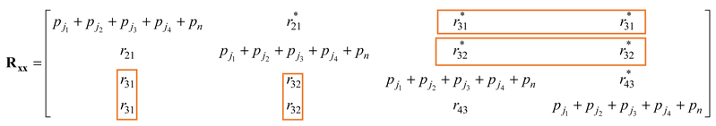
2. Array Signal Reception and Anti-Jamming Model

Signals received by each array element have different propagation delays and the delays appear in the form of phase differences. The steering vector of the signal is composed of the phase differences in a column containing signal DOA (direction of arrival) information in the spatial domain. Changes in the signal DOA might lead to changes in the steering vector. Matters such as element coupling and the inconsistency of radio frequency (RF) channels affect the measurement of phase difference, which worsens the anti-jamming performance. To simplify the analyses, this study ignores the non-ideal factors above and adopts the narrowband array signal model.

Assume that the navigation signal and interference signal are received by the N-element antenna array. The navigation signal, signal power, and steering vector are denoted as $s_i(t)$, $p_{s_i}$, $a_{s_i}$, respectively. The interference signal, interference power, and steering vector are denoted as $j_k(t)$, $p_{j_k}$, $a_{j_k}$, respectively. The thermal noise and noise power are denoted as $n_N(t)$ and $p_n$, respectively. “t” is the sampling time and the steering vector is a N × 1-dimensional column vector. The received signal of N-element array is

$$x(t)={\displaystyle \sum _{i=1}^I\sqrt{2p_{s_i}}{s}_i(t)a_{s_i}}+{\displaystyle \sum _{k=1}^K\sqrt{2p_{j_k}}{j}_k(t)a_{j_k}}+\sqrt{p_n}{n}_N(t)$$

(1)

where i represents the ith navigation signal, k represents the kth interference signal, and I and K denote the number of satellite signals and the number of jammers, respectively. $n_N(t)$ represents the noise signal column vector of the N-element array. This work concentrates on the condition that K ≥ N. The steering vector is the function of array geometry, antenna attitude $a_{antenna}$, and the signal’s incident DOA ($\theta$ in elevation, $\phi$ in azimuth). Assuming each element is isotropic and the array geometry is settled, the steering vector has the form

$$a={\left[\begin{array}{cccc}1& a_1(\theta ,\phi ,a_{antenna})& \cdots & a_{N-1}(\theta ,\phi ,a_{antenna})\end{array}\right]}^T$$

(2)

where a represents steering vector.

Denote the normalized coefficient of the spatial anti-jamming filter as $\overline{w}$. It is an N × 1-dimensional column vector. The output signal of spatial anti-jamming processing is

$$y(t)={\overline{w}}^{\mathrm{H}}x(t)$$

(3)

Since the intensity of interference and noise is much greater than that of navigation signals, the output residual interference-plus-noise power is approximately

$$p_{inres}={\overline{w}}^H{R}_{xx}\overline{w}$$

(4)

where $R_{xx}$ is the covariance matrix of the array signal. The computing of $R_{xx}$ is given later.

Correspondingly, the ICR (interference cancellation ratio) is defined to help evaluate the interference cancellation performance. The ICR is the ratio of input interference-plus-noise power and residual interference-plus-noise power.

$$ICR=\frac{{\displaystyle \sum _{k=1}^K{p}_{j_k}}+p_n}{p_{inres}}$$

(5)

The residual interference-plus-noise power is composed of two parts: residual interference power and noise power. Both of them have an impact on the signal CNR after the anti-jamming process. Equivalizing interference by noise, the equivalent CNR was developed to help analyze the impact of residual interference. It can be calculated as

$$CN{R}_{eq,dB}=-10\lg (\frac{p_n{B}_w}{p_{sout}}+\frac{p_{ires}/p_{sout}}{Q{R}_c})$$

(6)

where $B_w$ is the receiver bandwidth, $p_{sout}$ is the signal power after the anti-jamming process, $p_{ires}$ is the residual interference power, $R_c$ is the chip rate of the navigation signal, and $Q$ is the quality factor of interference. The increase of $p_{ires}$ leads to the decrease of $CN{R}_{eq,dB}$. If $CN{R}_{eq,dB}$ is smaller than the acquisition threshold, the acquisition fails and the receiver is unavailable.

The covariance matrix of the array signal is

$$R_{xx}=E\left\{x(t)x^{\mathrm{H}}(t)\right\}$$

(7)

where $E\{\cdot \}$ denotes expectation. Suppose the navigation signals, interferences, and noise are independent from each other, the interferences are stationary, and the interference intensities are much greater than the navigation signal. The covariance matrix of the received signal can be written as follows, where $R_{jj}$ and $R_{nn}$ are the interference covariance matrix and noise covariance matrix, respectively, and $I_N$ is N-dimensional unit matrix.

$$R_{xx}\approx {\displaystyle \sum _{k=1}^K{p}_{j_k}{a}_{j_k}{a}_{j_k}^{\mathrm{H}}}+p_n{I}_N=R_{jj}+R_{nn}$$

(8)

The covariance matrix can be constructed if the interference DOA, power, and noise power are known.

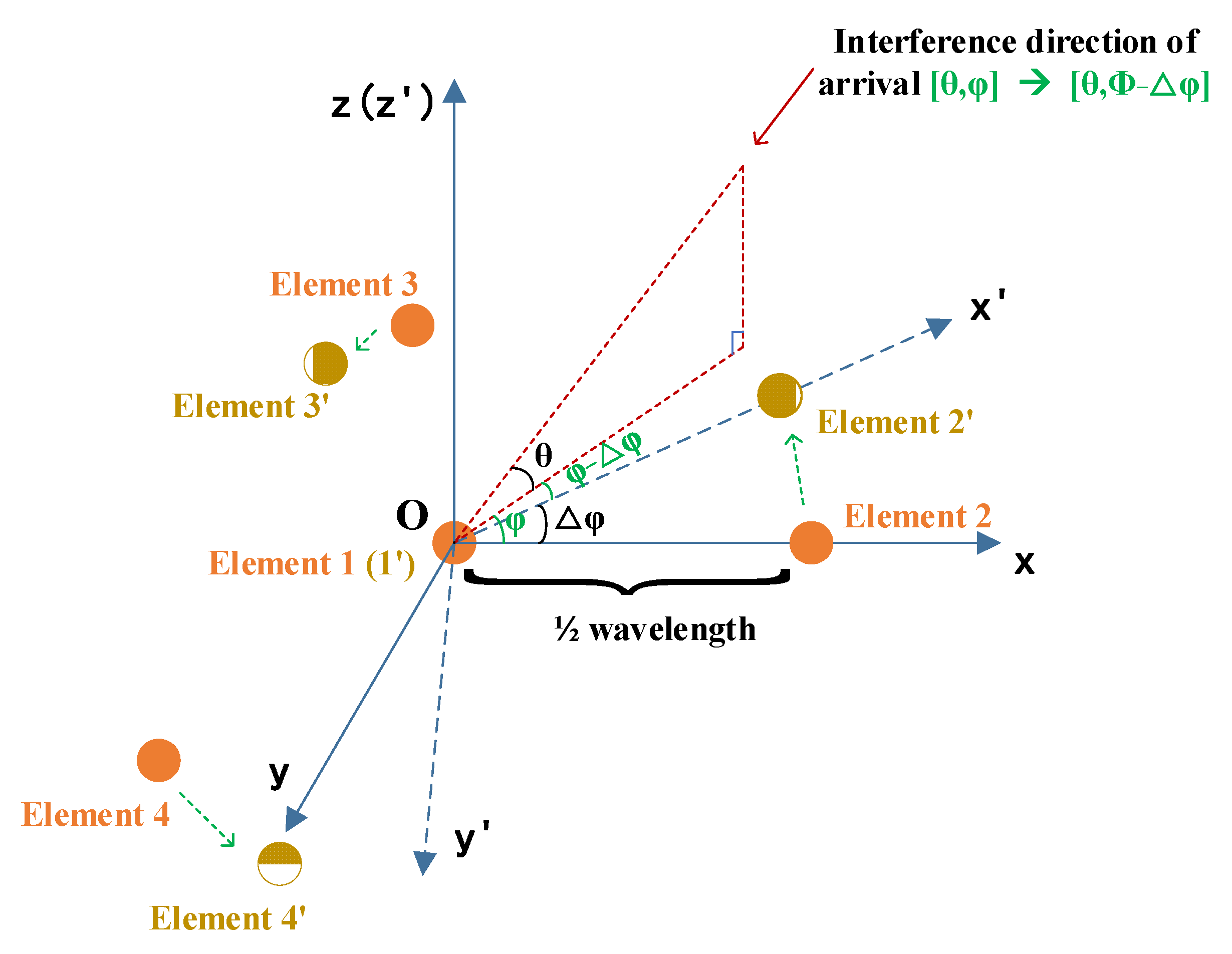
3. The Proposed Antenna Rotation Method

The rationale for the proposed method for sup-freedom jammers follows in this section. According to the Rayleigh entropy theorem, the minimum value of residual interference-plus-noise power is the minimum eigenvalue of covariance matrix, as in

$$p_{inres,\min }={\lambda }_{\min }[R_{xx}]$$

(9)

In this case, the normalized coefficient of the spatial anti-jamming filter $\overline{w}$ is the eigenvector corresponding to the minimum eigenvalue. If the interference does not surpass the array freedom, $\overline{w}$ is orthogonal to the interference steering vector $a_{j_k}$, and

$${\overline{w}}^{\mathrm{H}}{a}_{j_k}=0$$

(10)

So, the interference residual power is not affected by interference DOA. However, if the interference surpasses array freedom, the value of ${\overline{w}}^{\mathrm{H}}{a}_{j_k}$ is dependent on the correlation of the interference steering vectors. Thus, the residual interference-plus-noise power is a function of incident angles and interference powers.

$$p_{inres,\min }={\lambda }_{\min }[R_{xx}]=f(p_{j_k},{\theta }_{j_k},{\phi }_{j_k}|k=1,2,\cdots ,K)$$

(11)

At a certain moment, if the distances between the receiver platform and jammers are settled, the interference intensities are usually fixed. However, the incident angles can be changed by adjusting the antenna attitude. This can be utilized to reduce residual interference-plus-noise power.

In order to simplify the servo structure of the antenna, let the array antenna rotate along the normal direction of the array plane, and the rotation angle is $\Delta \phi$. As shown in Figure 2, xOy is the coordinate system of carrier platform and x’Oy’ is the coordinate system of the antenna array. The orange circles represent the array elements in coordinate xOy, and the yellow circles represent the locations of elements after antenna rotation. Suppose the interference DOA relative to the carrier platform is [θ, φ] and that the initial interference DOA relative to the antenna is [θ, φ]. After rotating the antenna array around the normal direction by angle Δφ, the interference DOA relative to the platform is still [θ, φ], while the DOA relative to antenna becomes [θ, φ−Δφ]. During the rotation of the antenna array, the relative relationship between interference steering vectors in the x’Oy’ coordinate have changed compared to that in the xOy coordinate. This leads to the change of the eigenstructure of the array signal covariance matrix, which further affects the residual power of the anti-jamming process.

In the course of antenna array rotation, the steering vector of the kth interference is

$$a_{j_k}=a({\theta }_{j_{k}0},{\phi }_{j_{k}0}+\Delta \phi )$$

(12)

where ${\theta }_{j_{k}0},{\phi }_{j_{k}0}$ is the initial elevation and azimuth angle of the kth interference. When ${\theta }_{j_{k}0},{\phi }_{j_{k}0}$ and the interference intensity are known and are constant, the received signal covariance matrix is only related to the rotation angle $\Delta \phi$. The interference-plus-noise residual power is a function of $\Delta \phi$, as in

$$p_{inres,\min }(\Delta \phi )={\lambda }_{\min }[R_{xx}(\Delta \phi )]$$

(13)

The rotation angle that makes the optimal residual interference-plus-noise power is

$$\Delta {\phi }_{opt}=\underset{\Delta \phi }{\arg \min } [p_{inres,\min }(\Delta \phi )]$$

(14)

For four- or seven-element arrays, the relationships between $p_{inres,\min }$ and incident angles are unclear, and it is hard to derive a simple expression of $\Delta {\phi }_{opt}=\underset{\Delta \phi }{\arg \min } [p_{inres,\min }(\Delta \phi )]$. Limited by the above reason, this section does not aim to figure out the detailed expression. An example of numerical calculation is given to help illustrate the proposed antenna rotation method.

Take the four-element central circular array as an example. The element locations are depicted in orange circles in Figure 2, and the element positions are given in

Table 2. Element positions of four-element central circular array.

Number of Elements	X	Y	Z
element 1	0	0	0
element 2	${\lambda }_c/2$	0	0
element 3	−${\lambda }_c/4$	−$\sqrt{3}{\lambda }_c/4$	0
element 4	−${\lambda }_c/4$	$\sqrt{3}{\lambda }_c/4$	0

. Figure 3a,b illustrate the ICR and residual interference power against rotation angle.

There are six interferences in Figure 3. The incident angles in azimuth are 28°, 9°, −2°, −42°, −56°, and −62°, respectively. In order to simplify the antenna pattern, the incident angles in elevation are 15°. The interference JSR (jam-to-signal ratio) are 60 dB. Because of the symmetry of the aforementioned array geometry, only the trend in the rotation angle 0°~60° is given here. The curve is extended periodically in the range of 0°~360°. It can be seen that at the rotation angle of 19°, the ICR reaches the optimal value and the interference residual power is the smallest. On the contrary, at the rotation angle of 47.7°, the ICR reaches the minimum and the residual interference power is the greatest. Figure 3c,d shows the antenna pattern at $\Delta \phi ={19}^{\circ }$ and $\Delta \phi ={47.7}^{\circ }$, respectively. The red dashed line indicates the equivalent incident angle after antenna rotation. In spite of both of the patterns having four nulls, the nulls in Figure 3c are formed closer to the incident directions while, in Figure 3d, the incident directions have a higher gain.

If there are enough satellite signals available, the eigenspace spanned by satellite signal steering vectors is similar to the unity matrix. The optimal anti-jamming performance can be obtained if the optimal rotation angle is determined.

4. The Variable-Step Iteration Algorithm for Efficient Determination of Optimal Rotation Angle

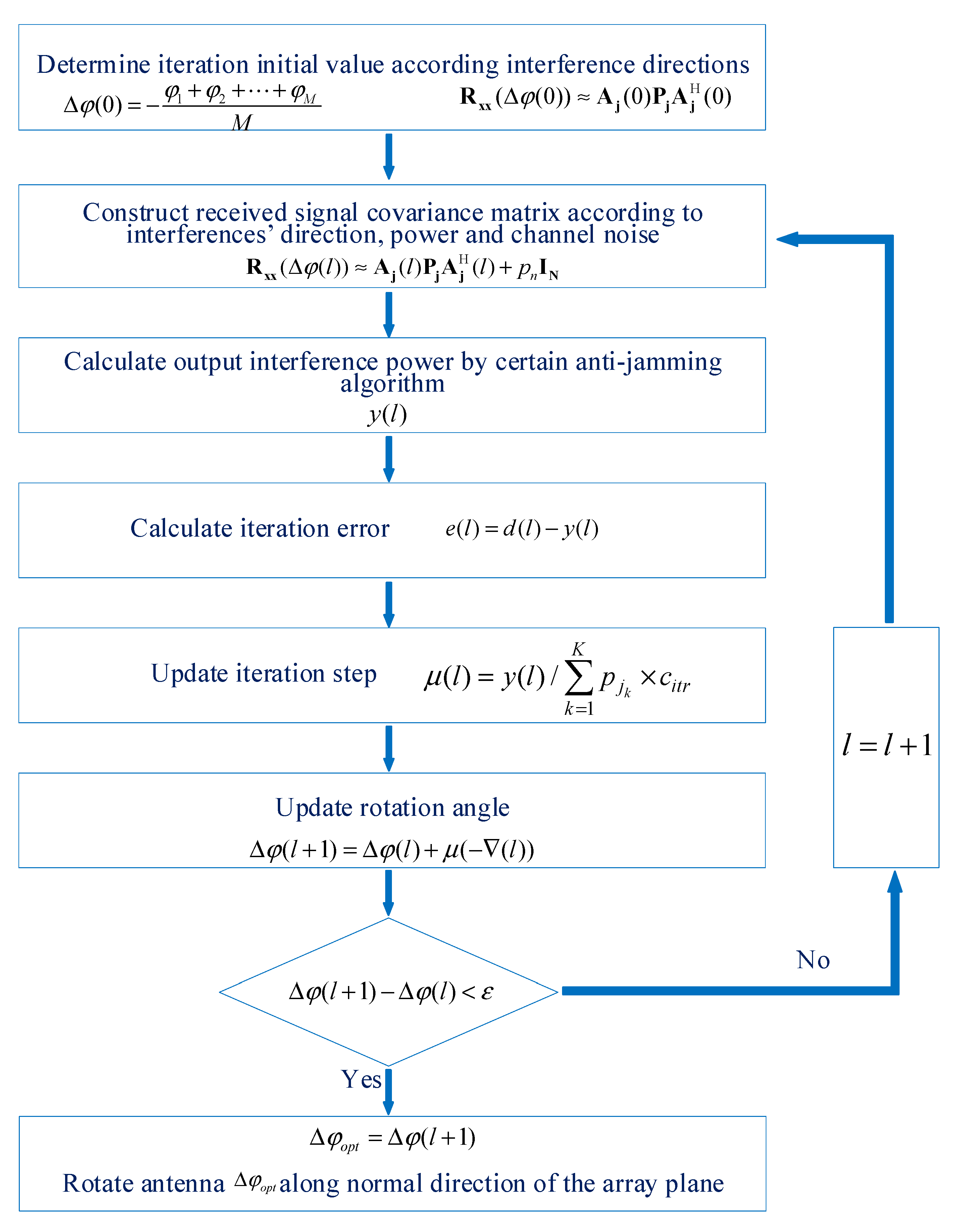
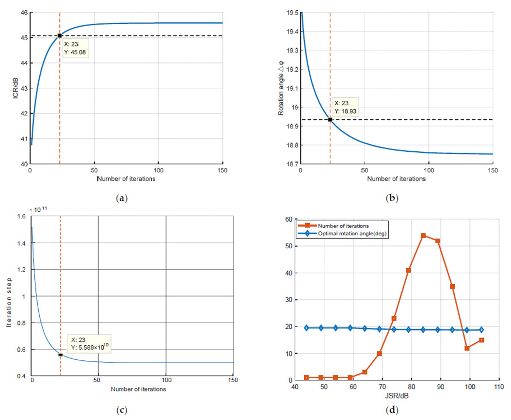
4.1. Iteration Process to Determine Optimal Rotation Angle

Because the mathematical expression of ${\lambda }_{\min }[R_{xx}(\Delta \phi )]$ is too complicated, it is hard to obtain $\Delta {\phi }_{opt}$ directly by Equation (14). Although one option is to traverse all possibilities of $\Delta \phi$ and find the optimal result, there is a contradiction between the computation amount and result resolution. Therefore, an iteration algorithm based on gradient descent was considered. The algorithm searches along the steepest descent direction of the residual interference-plus-noise power curve and updates $\Delta \phi$ according to the last iteration. The iteration is accomplished when the minimum residual power and the corresponding $\Delta {\phi }_{opt}$ is obtained.

The iteration based on gradient descent is shown in Formula (15). l represents the lth iteration, $y(l)$ is the residual interference-plus-noise power, $d(l)$ is the expected residual interference-plus-noise power, $e(l)$ is the error, and $\mu$ is the iteration step. Considering the interferences are expected to be completely suppressed while the noise power is close to zero, $d(l)$ was accordingly set to zero.

$$\{\begin{array}{l}y(l)={\lambda }_{\min }[R_{xx}(\Delta \phi (l))]\\ e(l)=y(l)-d(l) \\ \Delta \phi (l+1)=\Delta \phi (l)+\mu (l)\cdot (-\nabla (l))\end{array}$$

(15)

in which

$$-\nabla (l)=-\frac{\partial e(l)}{\partial \Delta \phi (l)}$$

(16)

and the Wiener solution of optimal $\Delta \phi$ is

$$\Delta {\phi }_{opt}=\underset{\Delta {\phi }_{opt}}{\arg }\frac{\partial e}{\partial \Delta \phi }=0$$

(17)

Suppose the incident direction and the power of interferences are known and the initial rotation angle is $\Delta \phi (0)$. A covariance matrix $R_{xx}(\Delta \phi )$ is constructed from the information of the interference intensity, incident direction, and rotation angle. The minimum residual interference-plus-noise power was obtained by eigen-decomposition. The error $y(l)$ equals to ${\lambda }_{\min }[R_{xx}(\Delta \phi )]$. For the problem that the error expression is too complicated for direct calculation $\nabla (l)$, the definition of a partial derivative is used to numerically approximate $\frac{\partial e}{\partial \Delta \phi }$, such that

$$\frac{\partial e}{\partial \Delta \phi }{|}_{\Delta \phi =\Delta {\phi }_l}=\underset{\Delta \to 0}{\lim }\frac{e(\Delta {\phi }_l+\Delta )-e(\Delta {\phi }_l)}{\Delta }$$

(18)

among which the anti-jamming algorithm in Formula (15-first equation) is not limited as above. It can be replaced by other algorithms, such as PI (power inversion) or MVDR (minimum variance distortionless response). As shown in Figure 3b, the curve of residual interference power has more than one extreme point. It is necessary to constrain the iteration step and initial value to avoid $\Delta \phi$ falling into a local optimum and to accelerate the convergence speed.

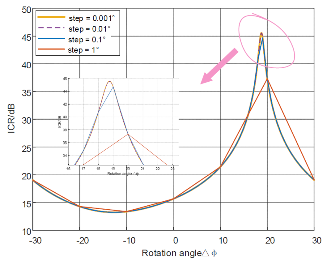
4.2. The Selection of Iteration Step

The convergence analysis of Formula (15) is as follows. Let the rotation angle error of the lth iteration be

$$v(l)=\Delta \phi (l)-\Delta {\phi }_{opt}$$

(19)

It can be written as

$$v(l+1)=v(l)+\mu (l)\cdot (-\frac{\partial e}{\partial \Delta \phi }{|}_{\Delta \phi =\Delta {\phi }_l})$$

(20)

When the iteration is convergent, it can be derived that

$$\underset{\Delta \phi \to \Delta {\phi }_{opt}}{\lim }[1-\frac{\mu (l)}{v(l)}\cdot \frac{\partial e(l)}{\partial \Delta \phi (l)}]=1$$

(21)

To guarantee $\underset{\Delta \phi \to \Delta {\phi }_{opt}}{\lim }v(l+1)=0$, the early stage of the iteration requires

$$\left|1-\frac{\mu (l)}{v(l)}\cdot \frac{\partial e(l)}{\partial \Delta \phi (l)}\right|<1$$

(22)

For the four-array central circular array antenna that is commonly used for navigation receivers, due to the symmetry and periodicity of the array, there would be

$$\max [|v(l)|]=\frac{\pi }{12}$$

(23)

if the initial value is selected reasonably. Considering that $v(l)$ and $\frac{\partial e(l)}{\partial \Delta \phi (l)}$ are both positive or negative, the iteration step should satisfy:

$$0<\mu (l)<|\frac{\pi }{6}/\frac{\partial e(l)}{\partial \Delta \phi (l)}|$$

(24)

In observing Figure 3b, the extreme values in $e(l)$ appear in the location of $\Delta \phi$ = 19° and $\Delta \phi$ = 47.7°, where only the former one is the optimal rotation angle. So, the iteration step also needs to meet the demand of being positively related to residual power. Then the iteration step is further required as:

$$\mu (l)=y(l)/{\displaystyle \sum _{k=1}^K{p}_{j_k}}\times c_{itr}$$

(25)

where input interference power ${\displaystyle \sum _{k=1}^K{p}_{j_k}}$ normalizes the residual power $y(l)$. $c_{itr}$ is a coefficient related to the iteration speed, whose empirical value can be selected by offline statistics of $\frac{\partial e(l)}{\partial \Delta \phi (l)}$. The statistics of $\frac{\partial e(l)}{\partial \Delta \phi (l)}$ is determined by implementation scenarios. This is discussed in Section 5.

4.3. The Selection of Initial Iteration Value

As shown in Figure 4, assume the number of interferences is K and their steering vectors are $a_{j_1}$, $a_{j_2}$, …, and $a_{j_K}$. According to matrix augmentation [18,19], it can be deduced that if the element on the diagonal is fixed, a covariance matrix with the follow form (please pay attention to the elements in orange boxes) has a relatively small minimum eigenvalue.

(26)

where r with subscript represents an element of the covariance matrix $R_{xx}$.

In order to approach $R_{xx}$ like this, let

$$\{\begin{array}{c}{\overline{w}}^{\mathrm{H}}{a}_{j_1}(\Delta \phi )\approx {\overline{w}}^{\mathrm{H}}{a}_{j_K}(\Delta \phi )\\ {\overline{w}}^{\mathrm{H}}{a}_{j_2}(\Delta \phi )\approx {\overline{w}}^{\mathrm{H}}{a}_{j_{K-1}}(\Delta \phi )\\ ⋮\end{array}$$

(27)

According to the symmetry of the array, if the interferences have the same intensity, one possible $\Delta {\phi }_{opt}$ is

$$\Delta {\phi }_{opt}\approx 0-\frac{{\phi }_{j_1}+{\phi }_{j_2}+\cdots +{\phi }_{j_K}}{K}$$

(28)

Otherwise, suppose the maximum interference power is $p_{j\max }$ and that M interference with power $p_{jm}\ge p_{j\max }/100$ is selected. The initial iteration value becomes

$$\Delta \phi (0)=-\frac{{\phi }_{j_1}+{\phi }_{j_2}+\cdots +{\phi }_{j_M}}{M}$$

(29)

In particular, for the four-element array, due to the periodicity of the residual power caused by the array geometry symmetry, initial iteration values can be adjusted by taking the remainder of $\frac{\pi }{6}$.

As a summary, the flow chart of the proposed algorithm is shown in Figure 5.

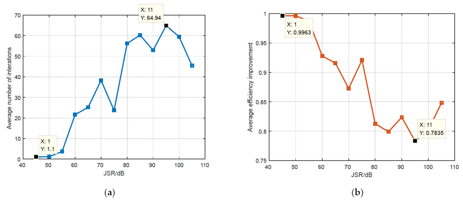
4.4. Evaluation of Iteration Efficiency

It is mentioned in Section 4.1 that there are two ways to get $\Delta {\phi }_{opt}$. One is to traverse all possible rotation angles (denoted as the “traversal algorithm”). Another one is the proposed variable-step iterative algorithm. In order to evaluate the efficiency of the proposed algorithm, the index of efficiency improvement is given below compared to the traversal algorithm.

Suppose the number of sufficient traversals is $N_s$ and the iteration number of the proposed algorithm is $N_i$. Taking $N_s$ as a benchmark, the efficiency improvement of the proposed algorithm is defined as

$$\eta =\frac{N_s-N_i}{N_s}\times 100\%$$

(30)

Although a fine angle resolution in traversal is always expected, the search time $N_s$ cannot be infinite. So, $N_s$ is considered sufficient while the ICR resolution meets the demand.

Because the anti-jamming algorithms usually contain eigen-decomposition or matrix inversion operations, the calculation amount of Formula (15) (first equation) is the largest in the iteration. Moreover, those operations are carried out twice in each iteration since the partial derivative of Formula (15) (third equation) is approximate by the numerical method. In order to more accurately evaluate the efficiency of the proposed algorithm, the equivalent iteration number is defined as twice the actual iterations, and Equation (30) is updated to

$$\eta =\frac{N_s-2N_i}{N_s}\times 100\%$$

(31)

5. Simulation Results and Analysis

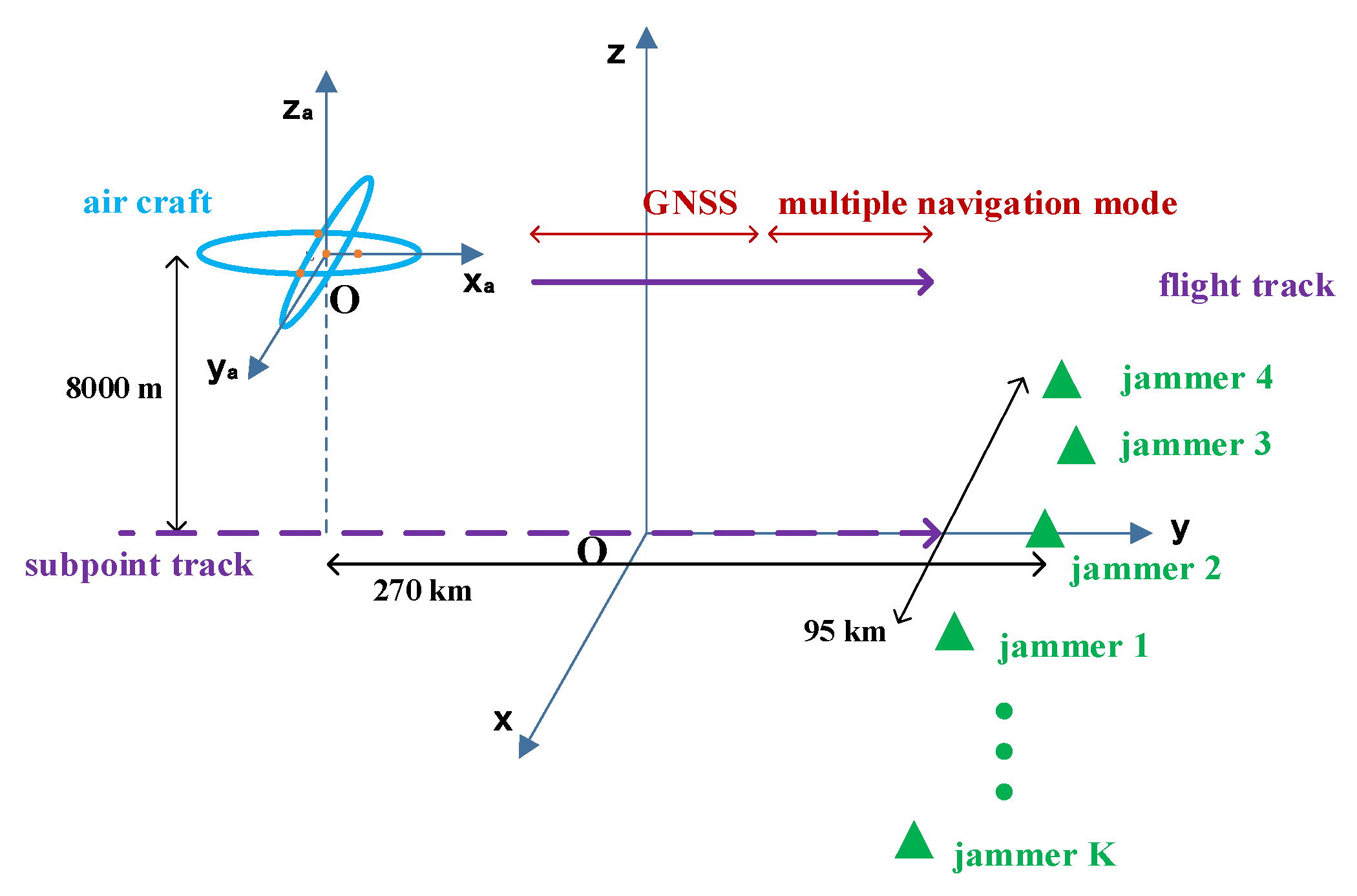
5.1. Simulation Scenario and Parameter Settings

As an example, a typical airborne scenario for distributed wideband interference was set for simulation. As shown in Figure 6, the orange points in the air craft are the receiver’s array elements and the jammers are located on ground. When the air craft approaches the jammers, there is a handing over of the guidance mode. While other navigation methods might be faced with error accumulation or weather influence, it is crucial to keep GNSS receivers available before the handing over.

This scenario determines the incident angle and received interference powers. A flight track of 270 km was set according to the flight height and earth curvature. If the length is longer than 270 m, the air craft and the jammers are invisible to each other in line of sight. A jammer distribution range along the x axis was set according to the practical scenario and 95 km in the figure above is an example. The air craft is at least 50 km from the jammers before the handing over of the navigation mode. The jammer incident angles in azimuth and elevation are shown in Figure 7a,b for the point in the simulation when the air craft flies over the jammers on the ground. During the initial period and midcourse of the flight, the approaching distance is much farther than the flight height, so the incident angles in elevation are no larger than 15°. The interference azimuth distribution $\Delta \Psi$ is defined as the maximum difference between interference azimuth angles and a typical value taken from Figure 7b is $\Delta \Psi \le {90}^{\circ }$. In the view that the distribution and number of jammers are usually uncertain, an assumption was made that the jammer incident angles are random and that they obey uniform distribution. Usually, the EIRP (equivalent isotropic radiated power) of jammers on the ground can be larger than 60 dBW. Considering the propagation loss, the JSR in Figure 7c is at 50 km. With the air craft shelter of around 20 dB, the JSR parameters in the simulation were set to 60~70 dB for each jammer.

On the basis of the above scenario, the Monte Carlo method was adopted in the simulation. The simulation parameters are shown in

Table 3. Simulation parameters.

Parameter	Value
light speed	3 × 108 m/s
carrier frequency	1268.52 MHz
array geometry	four element central circular array
array element spacing	1/2 wavelength
navigation signal power	−160 dBW
noise bandwidth	20.48 MHz
interference type	wideband gaussian noise
jammer incident angles in elevation	0°~−15°, uniform distribution
jammer incident angles in azimuth	0°~360°, uniform distribution
$\Delta \Psi$ of jammer incident angles in azimuth	90°
satellite signal incident angles in elevation	15°~90°, uniform distribution
satellite signal incident angles in azimuth	0°~360°, uniform distribution
number of interferences	4~30
implementation of anti-jamming algorithm	Sampling Matrix Inversion

. In addition, the carrier frequency of 1268.52 MHz is one of the central frequencies of the BeiDou Satellite Navigation System. It was taken as an example, while other GNSS carrier frequencies in the L-band obey the same analysis rules and have similar simulation results.

5.2. Effectiveness of Array Antenna Rotation Method

Based on the above scenario and parameters, the Monte Carlo simulation was repeated for 3000 times [20] to identify the effectiveness of the array antenna rotation method. As the simulation repeated, the DOAs of the interferences and satellite signals changed randomly as shown in Table 3. The JSR was set to 60 dB per jammer.

Ignoring the navigation signal DOA, Figure 8a shows the average residual interference-plus-noise power $p_{inres,\min }$ against the rotation angle and Figure 8b shows the corresponding average ICR. Taking the “4 jammer” blue line for instance, the residual interference power reaches the minimum value while the optimal rotation angle is 15°. At the same time, the ICR reaches the peak. The phenomenon is anastomotic with the analysis in Section 3. In order to make the figure clear, only the jammer number of 4~10 is given. The curves of more jammers are similar. They are analyzed later.

Considering the navigation signals, the proposed method was applied to the classic PI algorithm and MVDR algorithm. According to Equation (6), the numerical result of the anti-jamming output equivalent CNR is shown in Figure 9. The black dashed line represents the receiver’s acquisition threshold. As can be noted in Figure 9b, at the initial state for 4 jammers, the output CNR is around 23 dBHz, which does not satisfy the signal acquisition. As the antenna rotates, there is a segment for which the output CNR surpasses the threshold. In this segment, the receiver is available. Thus, the receiver can tolerate an interference intensity of at least a 60 dB JSR.

Furthermore, the index of the receiver’s anti-jamming capability is defined as follows: the receiver’s maximum tolerated interference power keeps the signal CNR greater than the receiver’s acquisition threshold. Assume that the CNR has a certain probability greater than the threshold. The probability here is the receiver availability and the interference power is recorded in the single-interference JSR.

Assume the receiver’s acquisition threshold has a CNR of 28 dBHz [21], the availability threshold is 95%, the interference number is 4~30, and the azimuth is $\Delta \Psi ={90}^{\circ }$. According to the incident direction statistics of terrestrial jammers relative to airborne GNSS receivers, the incident angle of jammers and satellite signals are listed in Table 3. Monte Carlo simulation is repeated 3000 times and the results are shown in Figure 10.

Figure 10a,b depicts the receiver’s anti-jamming ability. As analyzed in Section 2, the anti-jamming ability varies due to the antenna attitude (represented by rotation angle). For a fixed jammer number, the optimal anti-jamming ability is the greatest anti-jamming ability among all antenna attitudes in azimuth; it corresponds to the optimal rotation angle. As the jammer number increases, the optimal anti-jamming ability decreases. The decreasing rate gets lower when the jammer number is 12~30, so the lines in the figure are drawn in gray to simplify the figure. It can be seen that the optimal rotation angle changes slightly as the number of jammers increase.

The optimal anti-jamming improvement in Figure 10c,d indicates the difference between the greatest and the smallest anti-jamming ability for a fixed jammer number. It is the maximum anti-jamming improvement marked in Figure 10a. As the initial antenna attitude in practical applications is uncertain, the anti-jamming improvement floats in the interval [0, optimal anti-jamming improvement].

The performance of the proposed method can be concluded as follows. Under the condition of 4~30 jammers, the optimal anti-jamming ability improvement of the PI algorithm is 21~26 dB and the optimal anti-jamming ability is 44~61 dB (in the JSR of single interference, similarly hereinafter). The optimal anti-jamming ability improvement of the MVDR algorithm is 5~10 dB and the optimal anti-jamming ability is 47~61 dB after improvement.

5.3. Efficiency Evaluation of the Variable-Step Iteration Algorithm Based on Gradient Descent

Taking an application to the PI algorithm as an example, four interferences with different intensities were arbitrarily selected to validate the efficiency of the proposed implementation algorithm. The maximum azimuth intersection angle $\Delta \Psi$ = 90°. The interference parameters are shown in

Table 4. Interference parameters.

Interference Parameter	Angle in Elevation	Angle in Azimuth	JSR
Interference 1	−15°	28°	65 dB
Interference 2	−2°	18°	70 dB
Interference 3	−6°	−42°	62 dB
Interference 4	−10°	−62°	70 dB

and the other simulation parameters are the same as those in Table 3.

Figure 11 shows the relationship between the accuracy of the traversal algorithm and the search step size. In observing the partially enlarged map, it turned out that when the search resolution increases from 0.01° to 0.001°, the maximum value of the ICR varies slightly. Therefore, the maximum ICR corresponding to 0.001° search resolution was set as the theoretical optimal ICR. Under the interference parameters in Table 4, the theoretical optimal value of the interference suppression ratio is about 45.57 dB. The ICR error raised by implementation algorithm is defined as the difference between the maximum ICR and the theoretical optimal value. Requiring the ICR error to be less than 0.5 dB, the statistical search resolution was set to 0.1° and the search time turned out to be 600. This is taken as the benchmark $N_s$ in Formula (31).

Under the same interference parameters, the effect of the proposed implementation algorithm is shown in Figure 12a–c. The number of iterations is 23 when the iteration meets the aforementioned 0.5 dB demands. The corresponding optimal rotation angle is 18.93°. The iteration step in the process is shown in Figure 12c.

In the simulation, the empirical value of $c_{itr}$ in Equation (25) was determined by off-line statistics. Based on a great number of experiments, a possible $c_{itr}$ and an iteration step were obtained:

$$\mu (l)=\frac{y(l)}{({\displaystyle \sum p_{j_k}})\times {10}^{17.5-0.4616\lg (\frac{{\displaystyle \sum p_{j_k}}}{p_n})}}$$

(32)

From Equation (32), the iteration step is related to the total power of input interferences. Figure 12d shows the number of iterations and the optimal rotation angle under different JSR conditions.

In order to further illustrate the reasonability of $c_{itr}$ and the efficiency improvement of the proposed iteration algorithm, a Monte Carlo experiment was repeated 3000 times (the variables are interference DOAs). Please refer to Table 3 for jammer incident parameters. The calculated average iteration number is shown in Figure 13a. It reveals that the iteration step in Equation (32) meets the demand for a variety of jammer incident angles and intensities. Average efficiency improvement under different interference intensity conditions, as is shown in Figure 13b. It is depicted that the efficiency increase is 78.35–99.63%, which shows the algorithm has a positive effect on both strong and weak interferences.

6. Conclusions

This paper proposes an anti-jamming method and its implementation algorithm for GNSS receiver against sup-freedom interference. The major contributions are as follows:

(1)

In term of sup-freedom anti-jamming performance, the characteristic of direction-sensitivity is revealed;

(2)

Making use of the direction-sensitivity, an anti-jamming method based on array antenna rotation is proposed showing in which interference suppression is improved by rotating the antenna at a certain angle.

(3)

In order to determine the optimal rotation angle efficiently, an implementation algorithm of variable-step iteration is proposed. Meanwhile, we derived the criteria of the iteration initial value and step selection, which improve the iteration efficiency by over 78.35%.

There are several issues that should be taken into account in future works: (1) The algorithm presented in this paper assumes that the antenna array is ideal and ignores the mutual coupling of array elements and the inconsistency of RF channels. The influence of non-ideal factors will be further considered and the iterative formula will be modified accordingly when constructing the data covariance matrix. (2) A realistic scenario with live data will be needed to back up the findings. (3) Taking the receiver dynamic into account, the response speed of the antenna array servo structure needs to be considered. (4) It would be better to develop an equivalent algorithm in the data domain instead of adjusting the antenna attitude, which may avoid complex servo structures.

References

1. Kaplan, E.D.; Hegarty, C.J. GPS Principle and Application; Electronic Industry Press: Beijing, China, 2002; pp. 1–15. [Google Scholar]
2. Kohno, R.; Imai, H.; Hatori, M.; Pasupathy, S. Combinations of an adaptive array antenna and a canceller of interference for direct-sequence spread-spectrum multiple-access system. IEEE J. Sel. Areas Commun. 1990, 8, 675–682. [Google Scholar] [CrossRef]
3. Bei, D. Navigation Satellite System Open Service Performance Standard (Version 3.0). Available online: http://www.beidou.gov.cn/xt/gfxz/202105/P020210526216231136238.pdf (accessed on 21 March 2021).
4. Morton, Y.T.J.; van Diggelen, F.; Spilker, J.J., Jr.; Parkinson, B.W.; Lo, S.; Gao, G. Position, Navigation, and Timing Technologies in the 21st Century; Wiley-IEEE Press: Piscataway, NJ, USA, 2020; Volume 1, pp. 1121–1139. [Google Scholar]
5. Gupta, I.J.; Weiss, I.M.; Morrison, A.W. Desired Features of Adaptive Antenna Arrays for GNSS Receivers. Proc. IEEE 2016, 104, 1195–1206. [Google Scholar] [CrossRef]
6. Wang, J.; Ou, G.; Liu, W.; Chen, F. Characteristic Analysis on Anti-jamming Degrees of Freedom of GNSS Array Receiver. In Proceedings of the 13th China Satellite Navigation Conference, CSNC 2022, Beijing, China, 25–27 May 2022; pp. 463–472. [Google Scholar]
7. Fernandez-Prades, C.; Arribas, J.; Closas, P. Robust GNSS Receivers by Array Signal Processing: Theory and Implementation. Proc. IEEE 2016, 104, 1207–1220. [Google Scholar] [CrossRef]
8. Jie, W.; Wenxiang, L.; Feiqiang, C.; Zukun, L.; Gang, O. GNSS array receiver faced with overloaded interferences: Anti-jamming performance and the incident directions of interferences. J. Syst. Eng. Electron. 2022, 6, 1–7. [Google Scholar] [CrossRef]
9. Gstar Anti-Jam Gps—Electronic Protection. Available online: https://www.lockheedmartin.com/content/dam/lockheed-martin/rms/documents/electronic-warfare/GSTAR%20Brochure.pdf (accessed on 25 April 2022).
10. GPS Anti-Jam. Available online: https://www.mayflowercom.com/us/technology/gps-anti-jam/ (accessed on 25 April 2022).
11. Mitch, R.H.; Dougherty, R.C.; Psiaki, M.L.; Steven, P.P. Signal characteristics of civil GPS jammers. In Proceedings of the 24th International Technical Meeting of the Satellite Division of The Institute of Navigation (ION GNSS 2011), Portland, OR, USA, 20–23 September 2011; pp. 1907–1919. [Google Scholar]
12. Gu, Y.; Goodman, N.A. Information-Theoretic Compressive Sensing Kernel Optimization and Bayesian Cramér–Rao Bound for Time Delay Estimation. IEEE Trans. Signal Process. 2017, 65, 4525–4537. [Google Scholar] [CrossRef]
13. Moffet, A. Minimum-Redundancy Linear Arrays. Antennas and Propagation. IEEE Trans. Antennas Propag. 1968, 16, 172–175. [Google Scholar] [CrossRef]
14. Xu, Y.; Liu, Z.; Gong, X. Signal Processing of Polarization Sensitive Array; National Defense Industry Press: Beijing, China, 2013. [Google Scholar]
15. Ojeda, O.A.Y.; Grajal, J.; Lopez-Risueño, G. Analytical Performance of GNSS Receivers using Interference Mitigation Techniques. IEEE Trans. Aerosp. Electron. Syst. 2013, 49, 885–906. [Google Scholar] [CrossRef]
16. Li, W.; Mao, X.; Yu, W.; Yue, C. An Effective Technique for Enhancing Direction Finding Performance of Virtual Arrays. Int. J. Antennas Propag. 2014, 2014, 1–7. [Google Scholar] [CrossRef]
17. Brooks, D.H.; Nikias, C.L. The cross-bicepstrum: Definition, properties, and application for simultaneous reconstruction of three nonminimum phase signals. IEEE Trans. Signal Process. 1993, 41, 2389–2404. [Google Scholar] [CrossRef]
18. Horn, R.A.; Johnson, C.R. Matrix Analysis, 2nd ed.; Cambridge University Press: Cambridge, UK, 2012; pp. 164–177. [Google Scholar]
19. Mailloux, R.J. Covariance matrix augmentation to produce adaptive array pattern troughs. Electron. Lett. 1995, 31, 102–105. [Google Scholar] [CrossRef]
20. Junwei, N. Research on Anti-Jamming Algorithm and Performance Evaluation Technology of GNSS Antenna Array. Ph.D. Dissertation, National University of Defense Technology, Changsha, China, 2012. [Google Scholar]
21. Lu, Z.; Nie, J.; Chen, F.; Chen, H.; Ou, G. Adaptive Time Taps of STAP Under Channel Mismatch for GNSS Antenna Arrays. IEEE Trans. Instrum Meas 2017, 66, 2813–2824. [Google Scholar] [CrossRef]
Figure 1. Block diagram of the work.
Remotesensing 14 04774 g001
Figure 2. Antenna array rotation diagram.
Remotesensing 14 04774 g002
Figure 3. Relationship between antenna array attitude and anti-jamming performance. (a) ICR against rotation angle. (b) Residual interference power against rotation angle. (c) Antenna pattern at Δ φ = 19 . (d) Antenna pattern at Δ φ = 47.7 .
Remotesensing 14 04774 g003
Figure 4. The selection of initial iteration value.
Remotesensing 14 04774 g004
Figure 5. Iteration algorithm flow chart.
Remotesensing 14 04774 g005
Figure 6. Sketch map of airborne scenario.
Remotesensing 14 04774 g006
Figure 7. Jammer incident angles and JSR during the flight. (a) Incident angles in elevation. (b) Incident angle in azimuth. (c) JSRs increase as air craft gets closer to jammers.
Remotesensing 14 04774 g007
Figure 8. Simulation results ignoring navigation signal DOA. (a) Residual interference-plus-noise power against rotation angle. (b) ICR against rotation angle.
Remotesensing 14 04774 g008
Figure 9. Navigation signal CNR of anti-jamming output. (a) Applied in PI algorithm. (b) Applied in MVDR algorithm.
Remotesensing 14 04774 g009
Figure 10. Anti-jamming ability of rotating antenna array algorithm. (a) The anti-jamming ability of the PI algorithm for arbitrary (azimuth) antenna array attitude. (b) The anti-jamming ability of the MVDR algorithm for arbitrary (azimuth) antenna array attitude. (c) Array anti-jamming abilities and their maximum improvements applying the proposed method to the PI algorithm. (d) Array anti-jamming abilities and their maximum improvements applying the proposed method to the MVDR algorithm.
Remotesensing 14 04774 g010
Figure 11. Relationship between traversal accuracy and search step size.
Remotesensing 14 04774 g011
Figure 12. The effect of the proposed variable-step iteration algorithm. (a) The relationship between the ICR and the number of iterations. (b) The relationship between the optimal rotation angle and the number of iterations. (c) The relationship between the iteration step and the number of iterations. (d) The relationship between the number of iterations and the interference intensity.
Remotesensing 14 04774 g012
Figure 13. The reasonability of selected iteration step coefficient. (a) The relationship between the average iteration number and interference intensities. (b) The relationship between efficiency improvements and interference intensities.
Remotesensing 14 04774 g013