Atmospheric Correction Model for Water–Land Boundary Adjacency Effects in Landsat-8 Multispectral Images and Its Impact on Bathymetric Remote Sensing

Abstract

Atmospheric correction (AC) is the basis for quantitative water remote sensing, and adjacency effects form an important part of AC for medium- and high-spatial-resolution optical satellite images. The 6S radiative transfer model is widely used, but its background reflectance function does not take the radiance changes at water–land boundaries into account. If the observed land possesses bright features, the radiance of the adjacent water will be affected, leading to deviations in the AC results and increasing the uncertainty of water depth-based optical quantitative remote sensing. In this paper, we propose a model named WL-AE (a correction model for water–land boundary adjacency effects), which is based on the obvious radiance differences at water–land boundaries. This model overcomes the problem by which the background reflectance calculation is not terminated due to the highlighting pixel. We consider the influences of different $R_{ns}$ (neighborhood space) on the target pixel. The effective calculation of the equivalent background reflectance of the target pixel is realized, and the influence of the land area anomaly highlighting the pixel on the adjacent water is avoided. The results show that WL-AE can effectively improve the entropy and contrast of the input image and that the water–land boundary is greatly affected by adjacency effects, especially in the green and near-infrared bands, where the $M_{rc}$ (mean rate of change) are as high as 14.2% and 20.1%, respectively. In the visible wavelength, the $Sd$ of $R_{rc}$ (the relative rate of change) is positively correlated with $R_{ns}$, and the $Sd$ reaches 16.9%. Although the adjacency effect is affected by ground object types, its influence area remains within 3 km offshore. Based on the WL-AE and 6S results, the comparative test regarding bathymetric inversion shows that the influence is significant in the 0–5 m depth section. In Penang, the MRE of the 0–4 m inversion results is 31.4%, which is 10.5% lower than that of the 6S model.

1. Introduction

Atmospheric correction (AC) is of great significance for improving the quality of remote sensing images and accurately obtaining the true reflectance of ground objects. The AC of optical satellite images in the visible-to-NIR (near infrared) bands mainly includes atmospheric absorption, path radiation, and adjacency effects (AE) correction [1,2]. AE, which blurs and reduces the contrast of satellite images, is caused by atmospheric scattering between the ground and the sensor, where photons interact with objects around the target pixel and are then further scattered by the atmosphere into the sensor [3]. The current commonly used AC models assume that a uniform surface has the same reflectivity characteristics when performing AE correction, but the AE is significantly enhanced in areas with significant reflectance differences, especially at the water–land boundaries. In coastal areas, the optical complexity of seawater and the influence of nearby land increase AE [3,4]. Bathymetric optical remote sensing performs inversion by establishing a functional relationship between bathymetry and radiance (or reflectance) [5,6,7]. Therefore, the effective removal of AE is of great significance for water depth detection.

For decades, scholars have been trying to solve the effects caused by AE. In the initial stage, the contributions of background pixels were considered to be the same, so averaged the reflectance values of all pixels within a certain spatial range of the target pixel [8,9]. After that, it was found that the AE can be effectively removed by introducing the distance between the background pixels and the target pixel as the weight into the influence function [10,11,12,13]. It has been shown that the AE is directly affected by the optical thickness of both molecules and aerosols, so the weight function can be expressed as an environmental function, which fully takes the effects of the spatial distance and the optical thickness of molecules and aerosols into account [14,15].

As the mainstream radiative transfer (RT) model, 6S (Second Simulation of the Satellite Signal in the Solar Spectrum) has certain advantages, but it ignores the influence of radiance changes on the target pixel. Bulgarelli et al. [3,4,16,17] proposed a 3D-MC (three-dimensional Monte Carlo) algorithm by integrating the PSF (point spread function) with the role of multiple scattering according to a stratified atmosphere constrained by the coastal zone morphology. However, the correction results depend on the use of different statistical indices and different observation conditions [18]. Under ideal conditions, AE can affect waters up to 30 km offshore [3], but some researchers indicated that the effective value of $R_{ns}$ is about 1~2 km, or even smaller [12,15,19,20,21]. In addition, the specific range of its influence on quantitative remote sensing is still uncertain.

When correcting the AE of the coastal area, the ESA Medium Resolution Imaging Spectrometer (MERIS) and the NASA Moderate Resolution Imaging Spectroradiometer (MODIS) are used, and the sensors used include the Landsat-8 Operational Land Imager (OLI) and the ESA Sentinel-2 MultiSpectral Imagery (MSI) [3,22]. MERIS and MODIS are not suitable for quantitative water remote sensing due to their small spatial resolution. Although OLI and MSI mainly focus on land, they can also be used in the sea, and OLI can detect the information of the sea up to 36 km, while MSI is only 20 km [3]. In addition, the viewing geometry of the Sentinel-2 satellite (European Space Agency) causes it to be vulnerable to sun glint contamination, and the presence of sun glint significantly increases the difficulty of observing water-leaving radiance [23]. Landsat-8 has a good resolution (space, spectrum, and time, etc.) and effectively excludes the influence of water vapor at an 825 nm wavelength; and there are many data, easy to obtain, a wide range of applications, so this paper selected it for experiments.

Although AE correction models based on RT have been widely proposed, they are still in the stage of simulation and qualitative research [24,25,26]. Research on AE correction models for coastal waters has mainly focused on improving the contrast between water and land [27,28,29,30], and quantitative remote sensing research on the water is even less common. Investigations showed that the AC model affected the bathymetric inversion results, and 6S had a better advantage [31]. Based on 6S, this paper proposes a correction model for water–land boundary AE, named WL-AE. The model considers the obvious radiance difference at a water–land boundary region and incorporates a radiance ratio factor into the environmental function. Furthermore, a conditional function is added to solve the problem regarding the non-termination of the background reflectance calculation caused by highlighting pixels. The influence of $R_{ns}$ (the neighborhood space) on the target pixel is calculated. WL-AE can avoid the effects of high-brightness anomaly pixels on the equivalent background reflectance of the adjacent water column and realize effective calculation. To evaluate the effect of the WL-AE model on quantitative remote sensing, we applied it to water–land boundaries and performed depth inversion for coastal waters.

2. Correction Model for Water–Land Boundary AE

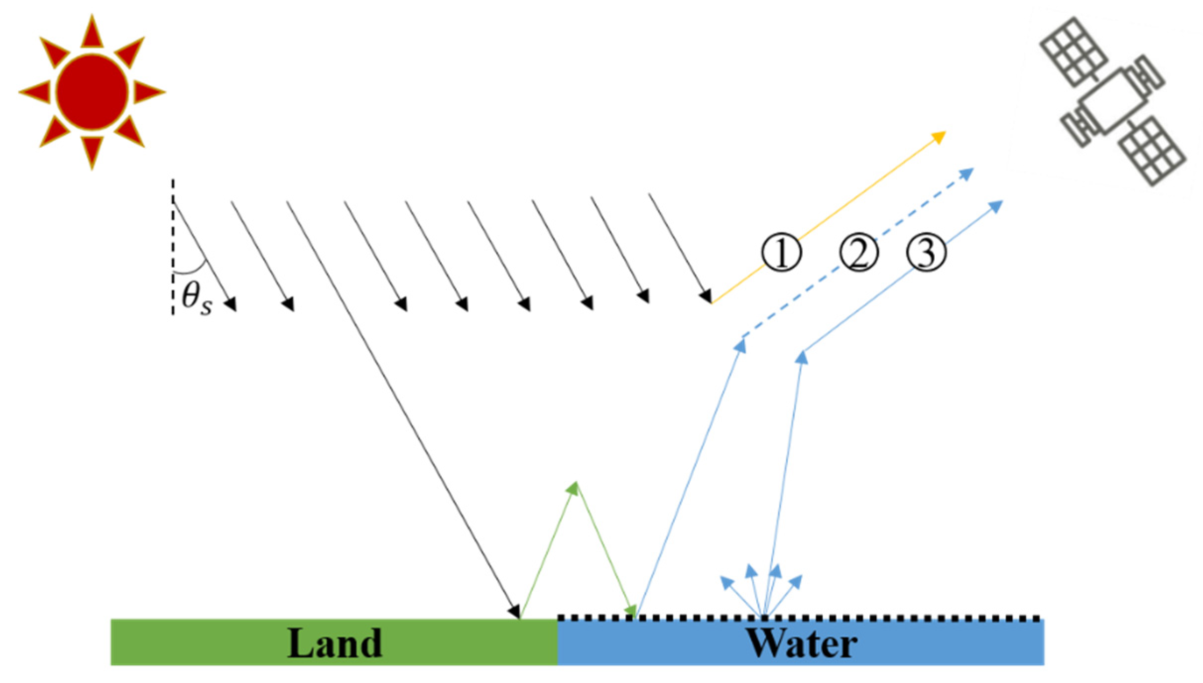
2.1. Composition of Remote Sensing Signals for Water Column

The radiance information received by the satellite sensor can be simplified as (1):

$$L_{tot}=L_{path}+L_{env}+L_{target},$$

(1)

where $L_{tot}$ is the total radiance by the target, $L_{path}$ is the path radiation, such as ① in Figure 1; $L_{env}$ is the ambient radiation, such as ② in Figure 1; and $L_{target}$ is the target radiance, such as ③ in Figure 1. At this point, $L_{target}=t·L_w$, t is the atmospheric diffuse transmittance; and $L_w$ is the water-leaving radiance. Equation (1) can be expressed as follows:

$$L_{tot}=t_g\left({\theta }_s,{\theta }_v\right)·\left[L_{path}+\frac{T\left({\theta }_v\right)·E_g\left(0\right)·{\rho }_t}{\pi \left(1-S·{\rho }_e\right)}+\frac{T{\left({\theta }_v\right)}^{diff}·E_g\left(0\right)·\left({\rho }_e-{\rho }_t\right)}{\pi \left(1-S·{\rho }_e\right)}\right],$$

(2)

where $t_g$ is the total atmospheric absorption transmittance; ${\theta }_v$ and ${\theta }_s$ are the observation zenith angle and the solar zenith angle, respectively; $T\left({\theta }_v\right)$ is the total atmospheric upward scattering transmittance; $T{\left({\theta }_v\right)}^{diff}$ is the total atmospheric upward diffuse scattering transmittance; $E_g\left(0\right)$ is the total solar radiance received by the ground at $\rho$ = 0; ${\rho }_t$ is the reflectance of the target; ${\rho }_e$ is the average background reflectance; and S is the hemispherical reflectance.

The 6S model assumes that the given surface is a non-uniform Lambertian and that there is no cloud. At this time, the apparent reflectance at the entrance pupil of the satellite can be expressed as (3).

$${\rho }^{*}\left({\theta }_s,{\theta }_v,\Delta \mathsf{\phi }\right)=t_g\left({\theta }_s,{\theta }_v\right)·\left[{\rho }_a\left({\theta }_s,{\theta }_v,\Delta \mathsf{\phi }\right)+\frac{T\left({\theta }_s\right)·\left[\exp \left(-\frac{\tau }{cos{\theta }_v}\right)·{\rho }_t+{\rho }_e·T\left({\theta }_v\right)\right]}{1-S·{\rho }_e}\right],$$

(3)

where ${\rho }^{*}$ is the apparent reflectance; ∆φ is the relative azimuth angle; ${\rho }_a$ is the path reflectance; τ is the total atmospheric optical thickness (AOT); $T\left({\theta }_s\right)$ is the total atmospheric downward scattering transmittance. The remote sensing reflectance ($R_{rs}$) of the target image element can be calculated using the 6S model. The aerosol types commonly used in the 6S model include continental, marine, and urban aerosol types.

2.2. Proposed Model

In coastal areas, the optical signal of the water column is affected by AE, which inevitably includes the scattering information of the terrestrial highlights, and their contributions cannot be ignored when performing quantitative remote sensing. The general 6S model assumes that the reflectivity of water is low and that the generated environmental irradiance ($E_{env}$) is small, so the influence of $E_{env}$ is ignored. The generation of water pixels has a negligible impact on the $R_{rs}$ of the target pixel; however, at the water–land boundary, the radiance (or reflectance) of each pixel changes abruptly due to the obvious changes in the ground objects. The radiance information derived from the highlighted land directly affects $L_w$ through the scattering of the atmosphere. For this situation, we propose WL-AE. The model optimizes the calculation function for ${\rho }_e$ to obtain the equivalent background reflectance (${\rho }_e^{final}$) and applies the radiance ratio $f$ between the background pixels and the target pixel to describe the influence of the reflectance difference between the target pixel and the background pixels on the radiance (or reflectance) of the target pixel. The calculation function is shown in (4):

$$\{\begin{array}{c}{\rho }_e^{final}\left(x_0,y_0\right)={{\displaystyle \sum }}_{x=x_0-\alpha }^{x=x_0+\alpha }{{\displaystyle \sum }}_{y=y_{0-\mathsf{\alpha }}}^{y=y_{0+\mathsf{\alpha }}}[\frac{{\rho }_{true}^{final}\left(x,y\right)·f·SR·F}{2\pi \sqrt{{\left(x_0-x\right)}^2+{\left(y_0-y\right)}^2}}]\\ F=\frac{f_R\left(SD\right)·t_d^R\left({\theta }_v,\lambda \right)+f_A\left(SD\right)·t_d^A\left({\theta }_v,\lambda \right)}{t_d^R\left({\theta }_v,\lambda \right)+t_d^A\left({\theta }_v,\lambda \right)}\\ f=\frac{L_{env}}{L_{target}}\\ \alpha =\frac{R_{ns}}{SR}\end{array},$$

(4)

where (x, y) is the pixel whose center is $\left(x_0,y_0\right)$ and whose spatial scale is the 2α neighborhood range; α is the number of pixels; ${\rho }_{true}^{final}$ is the final true reflectance of the target; SR is the spatial resolution of the sensor; SD is the spatial distance between the target pixel and the surrounding pixels; $t_d^R$ and $t_d^A$ are the upward diffuse scattering transmittance of atmospheric molecules and aerosols, respectively; $f_R\left(SD\right)$ and $f_A\left(SD\right)$ are calculated using the discretization function [21]; and $R_{ns}$ is the neighborhood space.

In the solution of ${\rho }_{true}^{final}$, it is necessary to calculate ${\rho }_e$, but due to the change in the ground object types adjacent to the water and land, there are abnormally bright pixel values in $R_{ns}$, which will fall into an infinite loop of computing of ${\rho }_e$. Given this problem, this paper proposes the following conditional function to limit the calculation to ensure that it progresses normally; see (5) and (6):

$$\left|{\rho }_{true}{\left(x_0,y_0\right)}^g-{\rho }_{true}{\left(x_0,y_0\right)}^{g-1}\right|\le \epsilon ,$$

(5)

$$M^g=M^{g-1},$$

(6)

where ${\rho }_{true}{\left(x_0,y_0\right)}^g$ is the target reflectance under ${\rho }_e{\left(x_0,y_0\right)}^{g-1}$; $\epsilon ={10}^{-5}$; M is the number of pixels that satisfy (5), and (6) means that the number of pixels that satisfy (5) is the same for the two iterations before and after (6), effectively avoiding the infinite loop caused by the image boundary and abnormal pixels, improving the operation efficiency.

The specific calculation steps of the WL-AE approach are as follows: the general 6S model is transformed to obtain the linear expression of the reflectance of the target pixel and background pixels:

$${\rho }_t=a-b·{\rho }_e,$$

(7)

Assuming that the surface is a uniform Lambertian surface, the reflectance ${\rho }_{uniform}$ of each pixel is calculated and expressed as the initial ${\rho }_e$, as shown in (8):

$${\rho }_{uniform}=\frac{a}{a·S+T\left({\theta }_s\right)·T\left({\theta }_v\right)},$$

(8)

Then, (8) is substituted into (7), and (9) is obtained by iterative calculation in a pixel-by-pixel manner:

$${\rho }_{true}{\left(x_0,y_0\right)}^g=a\left(x_0,y_0\right)-b\left(x_0,y_0\right)·{\rho }_e{\left(x_0,y_0\right)}^{g-1},$$

(9)

where,

$${\rho }_e{\left(x_0,y_0\right)}^{g-1}=\frac{1}{{\left(2\alpha +1\right)}^2}{{\displaystyle \sum }}_{x=x_0-\alpha }^{x=x_0+\alpha }{{\displaystyle \sum }}_{y=y_{0-\mathsf{\alpha }}}^{y=y_{0+\mathsf{\alpha }}}{\rho }_{true}{\left(x,y\right)}^{g-1},$$

(10)

Equations (5)–(10) are combined to calculate each pixel to obtain the target reflectance under the average background reflectance of each pixel, and this value is finally substituted into the equivalent background reflectance expression in (4). The real reflectance of the target under the equivalent background reflectance at this time can be obtained. The flowchart is shown in Figure 2. The AOT at 550 nm over the study area is first obtained using ACOLITE and brought into the 6S-AC model to obtain the parameters required for WL-AE, after which the ${\rho }_{true}^{final}$ is obtained by combining (4) to (10). The key of the WL-AE model is to achieve ${\rho }_e^{final}$, which is calculated using (9) and (10) until the condition (5) and (6) are satisfied, and finally, the obtained ${\rho }_e^{final}$ is substituted into (4) to achieve ${\rho }_{true}^{final}$.

3. Application and Analysis

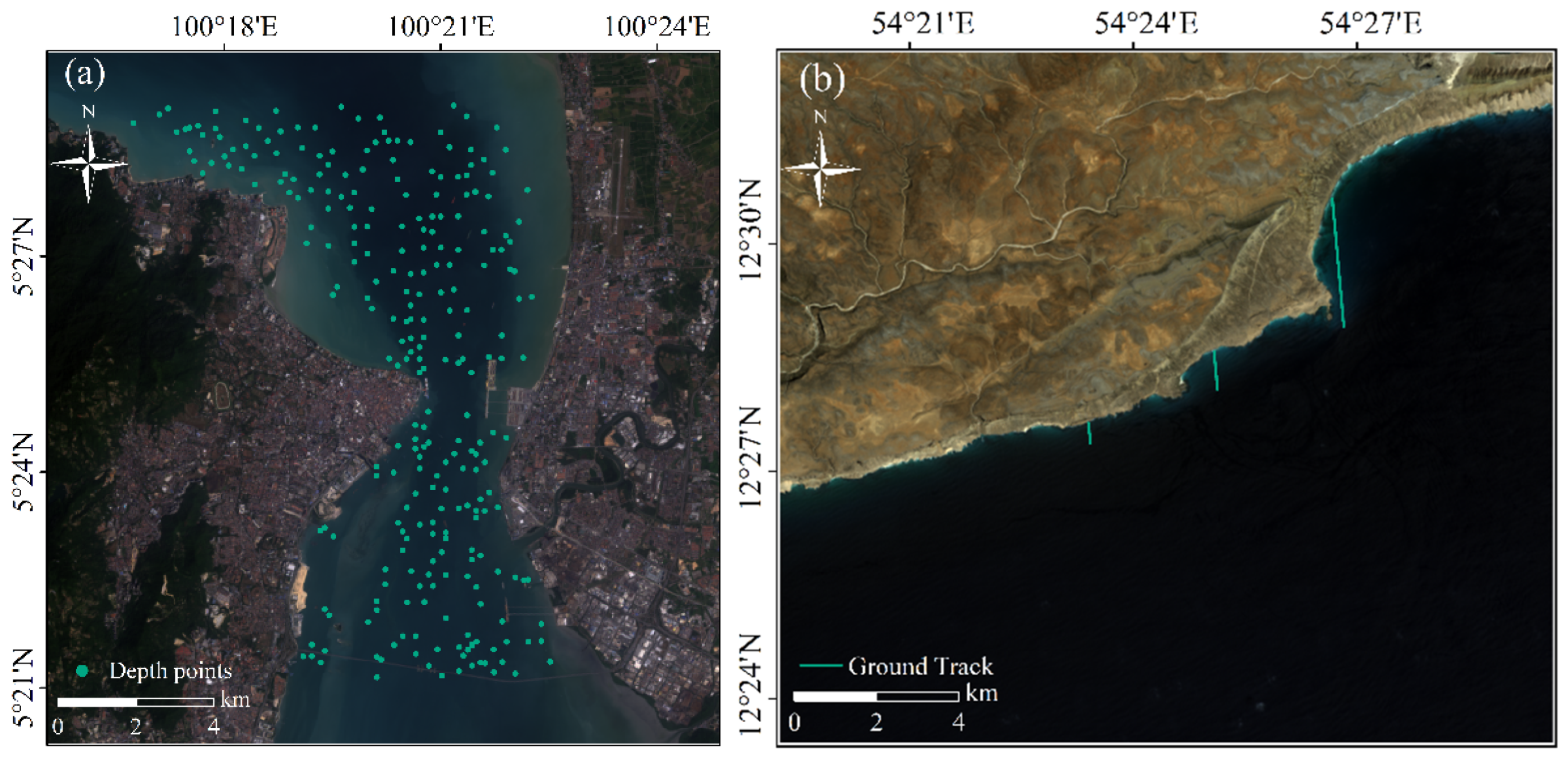
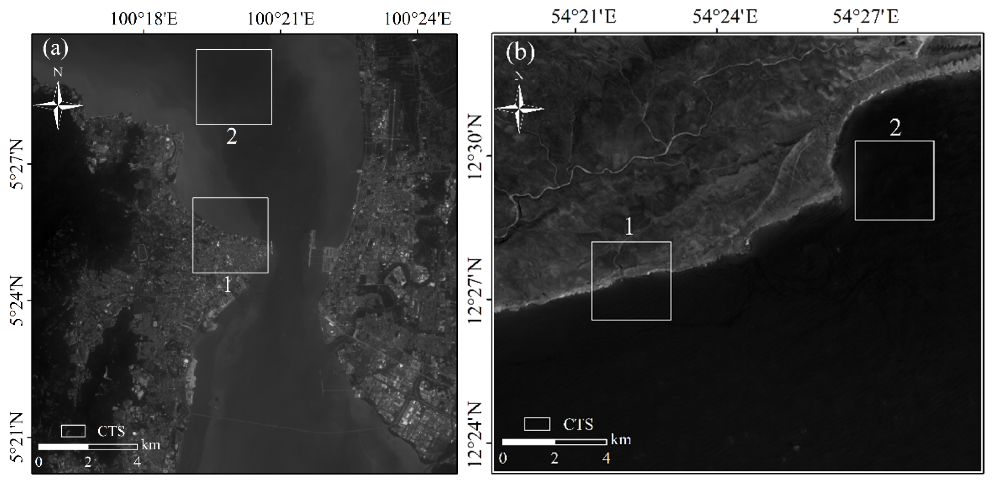
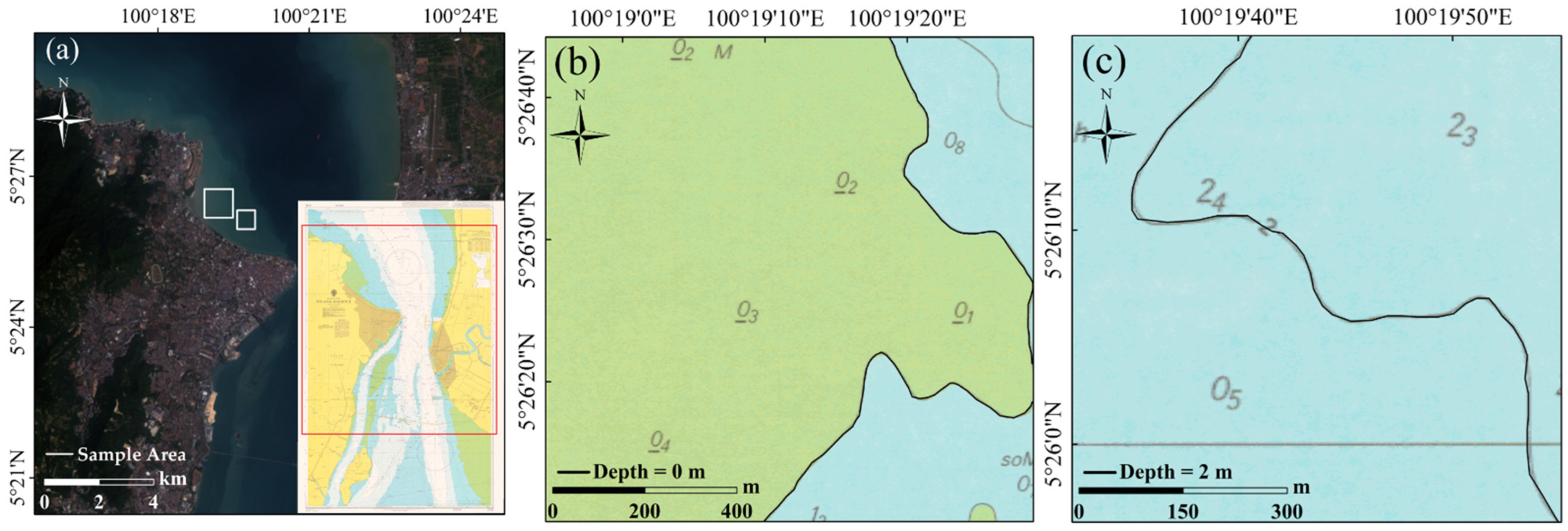
3.1. Data and Study Area

Penang is located in northwestern Peninsular Malaysia and is an important port city in George Town, the capital. It lies across the Strait of Malacca to the west of the Indonesian island of Sumatra. Socotra is located northwest of the Indian Ocean, near the Gulf of Aden. It belongs to the Socotra Province of Yemen. It is the main sea transportation route from the Indian Ocean to the Red Sea and East Africa. The land surface objects in the two study areas have the characteristics of high reflectivity, meeting the experimental requirements; the dates on which remote sensing images of the Penang and Socotra study areas were acquired are 26 January 2014 and 11 March 2021, respectively, as shown in Figure 3.

The bathymetric data for Penang were obtained from charts published in 2001 on a scale of 1:200,000, and they were georeferenced and geometrically corrected. The topographic data of ICESat-2 (Ice, Cloud, and Land Elevation Satellite-2) ATL03 acquired on 10 January 2020 were used for Socotra. ICESat-2 has three laser beams along the track direction, with a distance of 3.3 km across the orbit between adjacent beams and pulses emitted at 0.7 m intervals, for which the data accuracy can reach the decimeter level (https://Doi.org/10.5067/ATLAS/ATL12.005 (accessed on 28 December 2021)), and DBSCAN (Density-Based Spatial Clustering of Applications with Noise) has been used for ATL03 data in a previously developed algorithm for noise reduction.

3.2. Data Preprocessing and Bathymetric Inversion

Each Landsat-8 OLI image is a dimensionless value (DN value) that needs to be converted into absolute radiance for quantitative remote sensing inversion. The conversion equation is (11):

$$L_i=DN*gai{n}_i+offse{t}_i,$$

(11)

where $L_i$ is the i-band radiance and $gai{n}_i$ and $offse{t}_i$ are the i-band gain coefficient and offset coefficient, respectively. Furthermore, the ${\rho }^{*}$ of the given OLI image can be calculated by (12):

$${\rho }^{*}=\frac{M*DN+A}{cos{\theta }_s},$$

(12)

where $M$ is the multiplicative reflectance scaling factor and $A$ is the additive reflectance scaling factor. Among them, $gai{n}_i$, $offse{t}_i$, $M$, and $A$ can be obtained from the Landsat-8 metadata.

The aerosol model used for urban Penang contained 29% water-soluble particles, 70% dust-like particles, and 1% soot particles. The aerosol model used for Socotra is Marine, consisting of 5% water-soluble particles and 95% marine particles.

Bathymetric optical remote sensing performs inversion by establishing a functional relationship between bathymetry and radiance (or reflectance) [5,6,7]. In this paper, the multiband log-linear model is chosen for bathymetric inversion, and the model considers that the reflectance ratio of the bands is constant over different substrate types [7]. The model obtains the expression between water depth and reflectivity at the control points by regression and applies it to the global image. The visible wavelength has the largest atmospheric transmittance and the smallest water attenuation coefficient, which is the best spectral range of bathymetric inversion. Although sunlight is almost completely absorbed in the NIR band, part of the signal is still retained [32]. Therefore, to improve the accuracy of water depth inversion, the model adopts visible-to-NIR bands. The formula is:

$$Z=a_0+{{\displaystyle \sum }}_{i=1}^n{a}_{i}ln\left[R_{rs}\left({\lambda }_i\right)-R_{rs}{}_{\infty }\left({\lambda }_i\right)\right],$$

(13)

where $a_0$ and $a_i$ are constants, n is the number of spectral bands; $R_{rs}\left({\lambda }_i\right)$ is the i-band reflectance value, and $R_{rs}{}_{\infty }\left({\lambda }_i\right)$ is the i-band reflectance in deep water. The tidal height at the time of water depth acquisition is not the same as the tidal height at the time of remote sensing image acquisition. To make the bathymetric inversion results more accurate, tidal correction should be applied to the measured depth data. The principle is that the depth value at a certain moment is equal to the measured value plus the tidal height at that moment, and the tidal heights at the imaging moments of Penang and Socotra are 0.9 m and 1.3 m, respectively, while it is 1.8 m when obtained by ICESat-2 (TIDES4FISHING|Tide times, tide tables, and solunar charts for fishing).

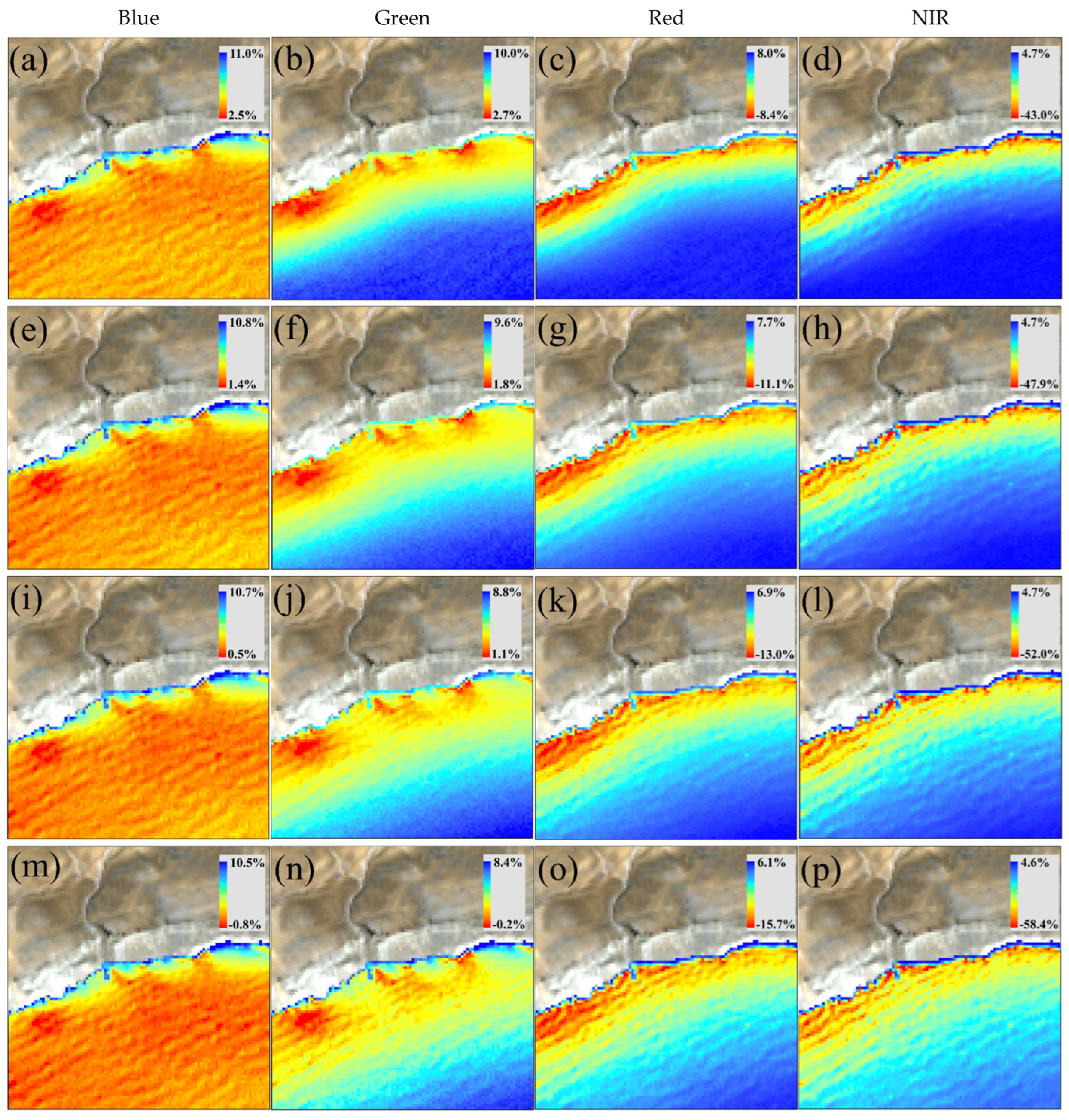
3.3. Analysis of the AC Results

The size of $R_{ns}$ in WL-AE directly affects the correction results, and this value can be replaced by the number of pixels, which can be expressed as the ratio of the spatial distance from the target pixel to the background pixels and the SR of the image. Since the size of $R_{ns}$ directly affects the removal effect of AE and considering the SR of OLI images, the selected $R_{ns}$ values are 1 km, 1.5 km, 2 km, and 3 km, so α is 33, 50, 67, and 100. respectively.

3.3.1. Overall Quality Assessment

Histograms of the 6S and WL-AE correction results were plotted, and the images were analyzed using entropy and contrast. Entropy represents the chaos degree of the grayscale and reflects the richness of image information, while contrast can reflect the details of the image [23]. The entropy and contrast are shown in Equations (14) and (15), in which P(ψ) indicates the occurrence probabilities of different gray levels in the image.

$$Entropy=-{{\displaystyle \sum }}_{\psi }P\left(\psi \right)logP\left(\psi \right),$$

(14)

$$Contrast=\frac{Max\left({\rho }_t\right)-Min\left({\rho }_t\right)}{Max\left({\rho }_t\right)+Min\left({\rho }_t\right)},$$

(15)

The reflectance histograms of Penang are shown in

Table 1. Reflectance Histogram of Penang.

Model	Blue	Green	Red	NIR
6S
WL-AE (1 km)
WL-AE (1.5 km)
WL-AE (2 km)
WL-AE (3 km)

. The visual interpretation shows that WL-AE effectively increases the contrast levels of remote sensing images. On the whole, the histograms of the 6S and WL-AE results have the same trend, but the histogram of WL-AE is smoother than that of 6S. In the visible wavelength range, the peak value of the histogram moves to the left and approaches 6S with increasing $R_{ns}$. For example, the peak reflectance of 6S in the blue band appears at reflectance position 1000, while the peak values of WL-AE in the blue band under different $R_{ns}$ appear at 1150, 1130, 1108, and 1088. In addition, the reflectance in the visible wavelength range is mainly in [500, 1500], and there are double peaks in the red band. The NIR band is mainly used for land–water differentiation, and it is clear from Table 1 that the NIR band is greatly affected by adjacent pixels. In this wavelength range, the peak reflectance of the 6S model is approximately 323, while the peak values of the four results of the WL-AE model are approximately 352, 327, 293, and 267. With the increase in $R_{ns}$, the peak value of the visible band gradually approaches that of 6S and becomes greater than that of 6S. When $R_{ns}$ is 1.5 km in the NIR band, the peak reflectance is the same as that for 6S.

The entropy and contrast levels of the Penang and Socotra images in each band are shown in

Table 2. Evaluation of the AC Results.

Region	Band	Blue		Green		Red		NIR
	Model	Entropy	Contrast	Entropy	Contrast	Entropy	Contrast	Entropy	Contrast
Penang	6S	2.045	0.880	2.067	0.883	2.051	0.924	2.010	0.922
	WL-AE (1 km)	2.180	0.904	2.182	0.886	2.182	0.924	2.182	0.970
	WL-AE (1.5 km)	2.182	0.906	2.182	0.888	2.182	0.926	2.182	0.990
	WL-AE (2 km)	2.182	0.907	2.182	0.889	2.182	0.927	2.182	1.000
	WL-AE (3 km)	2.182	0.909	2.182	0.892	2.182	0.928	2.182	1.018
Socotra	6S	2.075	0.831	2.089	0.883	2.097	0.936	2.101	0.969
	WL-AE (1 km)	2.182	0.856	2.182	0.881	2.182	0.934	2.182	1.047
	WL-AE (1.5 km)	2.182	0.859	2.182	0.881	2.182	0.934	2.182	1.063
	WL-AE (2 km)	2.182	0.861	2.182	0.882	2.182	0.939	2.182	1.076
	WL-AE (3 km)	2.182	0.864	2.182	0.883	2.182	0.948	2.182	1.093

. It was found that the entropy and contrast of each band of 6S were lower than those of WL-AE, the information richness of the image obtained after utilizing WL-AE is significantly improved, and the NIR band is significant. The entropy and contrast of Penang in the NIR band increase by 0.172 and 0.096, respectively. The contrast increases by 0.124 in the NIR band of Socotra, which provides a basis for effectively distinguishing the boundary between land and water. The entropy increment gradually decreases with increasing wavelength, and the corresponding $R_{ns}$ gradually decreases when it reaches a stable value, especially in the blue and NIR bands. When $R_{ns}$ = 1 km in Penang, the contrast levels of the images in both the blue and NIR bands are improved by 0.024 and 0.048, respectively, over those of 6S. However, when $R_{ns}$ is 2 km and 3 km, the contrast changes are only 0.002 and 0.018, which are only 1/12 and 3/8 of the previous values. In the blue and NIR bands of Socotra, the increase rate of the contrast gradually decreases with increasing $R_{ns}$. When $R_{ns}$ is 1 km and 3 km, the contrast increments of the two bands relative to 6S are 0.025, 0.033, and 0.078, 0.124, respectively.

3.3.2. Regional Quality Assessment

The core research of this paper concerns the AE of the water–land boundary regions. To better test the practicability of the proposed model, the water pixels of two CTSs (characteristic test sample) at the water–land boundary region (Mixed Zone) and only the water column (Water Zone) are selected for quantitative analysis, as shown in Figure 4.

The $R_{rc}$ (relative rate of change), $M_{rc}$ (mean rate of change), and $Sd$ (standard deviation) are used to quantify the CTSs. The above indices can vividly represent the relative differences between each pixel of the two models and the degree of dispersion of the changes. As shown in Equations (16)–(18), $n$ represents the number of water pixels in the CTS.

$$R_{rc}\left(x,y\right)=\frac{{\rho }_{WL-AE}\left(x,y\right)-{\rho }_{6S}\left(x,y\right)}{{\rho }_{6S}\left(\mathrm{x},\mathrm{y}\right)},$$

(16)

$$Mrc=\frac{{{\displaystyle \sum }}^{ }\left|R_{rc}\left(x,y\right)\right|}{n},$$

(17)

$$Sd=\sqrt{\frac{{{\displaystyle \sum }}_{i=1}^n{\left(R_{rc}\left(x_i,y_i\right)-MRC\right)}^2}{n-1}},$$

(18)

As shown in Figure 5, within the Mixed Zone of Penang, the value of the $R_{rc}$ span shows a trend of decreasing, and it increases with increasing wavelength. With the increase in $R_{ns}$ in the same band, $R_{rc}$ gradually decreases, but the variation range increases gradually. When $R_{ns}$ = 1 km, the $R_{rc}$ interval spans of the four bands are 5.1%, 4.7%, 11.4%, and 54.6%. When $R_{ns}$ = 3 km, the $R_{rc}$ interval spans of the four bands are 6.2%, 5.9%, 12.1%, and 71.4%, respectively. The variation in $R_{rc}$ in the visible wavelength range is similar to that of the original image water surface state, but the distribution of $R_{rc}$ in the NIR band shows an obvious “step”; i.e., the distribution of $R_{rc}$ is parallel to the shoreline and related to the offshore distance. The pixel values near the shore mainly exhibit a downward trend, with a maximum decrease of 68.6%, and gradually increase with increasing offshore distance. This indicates that there are differences between the responses of different wavebands to land features, and different wavebands are affected by AE.

Similar to Penang, Socotra also shows a trend of decreasing and then increasing $R_{rc}$ span values with the increasing wavelength in the Mixed Zone, and the inflection point appears in the green band. With the increase in $R_{ns}$ in the same band, $R_{rc}$ gradually decreases, but the range of variation increases gradually. The relative change rate ranges of the red band under different $R_{ns}$ values are 16.4%, 18.8%, 19.9%, and 21.8%, and those of the NIR band are more obvious. It can be seen from Figure 6 that the $R_{rc}$ at the water–land mixture is larger, mainly due to not only AE but also the influence of mixed pixels. $R_{rc}$ shows a clear “step”; that is, the distributions of $R_{rc}$ and the shoreline show parallelism and are related to the offshore distance. In the visible wavelength, $R_{rc}$ decreases with increasing offshore distance. This is different from Penang, indicating that AE is not only related to the wavelength but also closely related to the types of features and the water quality in the study area.

As seen in

Table 3. Analysis indices of the CTS Correction Results Obtained Under Different $R_{ns}$ Values.

Study Area	Samples		Mixed Zone				Water Zone
	Model	Index	Blue	Green	Red	NIR	Blue	Green	Red	NIR
Penang	WL-AE (1 km)	$M_{rc}$/%	12.5	14.2	10.3	8.2	11.5	16.5	13.9	7.3
		$Sd$/%	0.7	0.6	1.8	6.6	0.4	0.7	0.7	0.8
	WL-AE (1.5 km)	$M_{rc}$/%	10.7	12.8	8.7	10.1	9.7	15.0	12.9	6.7
		$Sd$/%	0.9	0.5	1.9	9.1	0.4	0.7	0.7	0.8
	WL-AE (2 km)	$M_{rc}$/%	9.4	11.8	7.5	13.1	8.5	14.0	12.1	6.0
		$Sd$/%	1.0	0.6	1.7	10.7	0.5	0.8	0.9	1.5
	WL-AE (3 km)	$M_{rc}$/%	7.5	10.4	5.6	20.1	6.4	12.1	10.1	4.6
		$Sd$/%	1.2	0.7	1.5	11.7	0.6	0.8	1.1	3.1
Socotra	WL-AE (1 km)	$M_{rc}$/%	4.4	7.8	5.0	5.4	3.8	11.0	10.1	4.8
		$Sd$/%	0.8	1.6	2.4	4.8	0.5	1.0	0.9	1.2
	WL-AE (1.5 km)	$M_{rc}$/%	4.5	6.6	4.0	6.6	3.0	10.3	9.2	4.8
		$Sd$/%	1.0	1.6	2.1	6.5	0.5	1.2	1.8	4.8
	WL-AE (2 km)	$M_{rc}$/%	2.7	5.6	3.4	8.5	2.4	9.6	8.1	6.1
		$Sd$/%	1.1	1.5	2.1	7.4	0.5	1.5	2.9	9.0
	WL-AE (3 km)	$M_{rc}$/%	1.4	3.9	3.6	13.3	1.1	7.8	4.6	12.0
		$Sd$/%	1.4	1.3	2.9	7.7	0.7	2.0	5.0	16.9

, AE has different responses to different wavelengths. For both Penang and Socotra, the $M_{rc}$ changes in the two CTSs in the visible wavelength are different due to surface object type differences, but the changes show a trend of rising first and then decreasing with the increase in wavelength, and the green band changes the most. The $M_{rc}$ at the visible wavelength decreases with increasing $R_{ns}$; the $M_{rc}$ in the two CTSs at $R_{ns}$ = 1 km in Penang are 12.5% and 11.5%, respectively, which are 5.0% and 5.1% higher than the $M_{rc}$ at $R_{ns}$ = 3 km. The change rate of the blue band in the water–land boundary is larger than that in the water-only area, and the fluctuation is more obvious. When $R_{ns}$ is the same, the $M_{rc}$ difference between the two CTSs in Penang is approximately 1.0%, but the $Sd$ difference gradually increases. When $R_{ns}$ = 1 km, the $Sd$ differences are 0.3% and 0.6%, respectively. The variation patterns of the two study areas in the NIR band remain consistent, i.e., the $Sd$ is positively correlated with $R_{ns}$. The difference between the two CTSs in Penang is obvious, and the variability and volatility of the Mixed Zone are significantly greater than those of the Water Zone. When $R_{ns}$ = 3 km, the $M_{rc}$ of the two CTSs are 20.1% and 4.6%, respectively, with a difference of 15.5%. At this time, the $Sd$ of the Mixed Zone is 11.7%, which is 8.6% higher than that of the Water Zone. In Penang, both the $M_{rc}$ and $Sd$ of the water–land mixed area are larger than those of the water–only area, and the gap between the two CTS values gradually increases with increasing $R_{ns}$. However, in Socotra, the $M_{rc}$ of the Mixed Zone is greater than that of the Water Zone, but when $R_{ns}$ > 1.5 km, the $Sd$ of the Water Zone is larger than that of the Mixed Zone; for example, when $R_{ns}$ = 2 km, the $Sd$ of the CTSs are 7.0% and 9.0%, respectively.

3.4. Analysis of the Bathymetric Inversion Results

The 6S and WL-AE results are quantitatively inverted concerning the water depth from both the overall and segmented perspectives, and the results are analyzed. The evaluation factors used are the MAE (mean absolute error) and MRE (mean relative error); see (19) and (20). Where $Z^{\prime }$ is the inversion of the obtained depth value and Z is the original depth value. The selected depth range is 20 m, and the segment interval is 5 m.

$$MAE=Mean\left({{\displaystyle \sum }}^{}\left|Z^{\prime }-Z\right|\right),$$

(19)

$$MRE=Mean\left(\frac{{{\displaystyle \sum }}^{}\left|Z^{\prime }-Z\right|}{Z}\right)·100\%,$$

(20)

3.4.1. Assessment Analysis of the Overall Inversion Accuracy

As shown in Figure 7, the difference in accuracy between the bathymetric inversion results corresponding to WL-AE and 6S is small. In Penang, the MAE and MRE of the 6S inversion results are 3.02 m and 37.3%, respectively, and the difference between the MRE of the inversion results of the two correction models is within 1.5%. For Socotra, it can be found that the accuracies of the inversion results of the two correction models are consistent. Studies have shown that as the distance between the background pixels and the target pixel increases, the AE, caused by the background image radiance reaching the target pixel after repeated scattering by the atmosphere, gradually decreases [9,10]. Additionally, the depth and the offshore distance show a positive correlation, which enables the AE to affect the limited depth, so segmented inversion and accuracy analyses are performed to further explore the effect of AE on the optical remote sensing bathymetry.

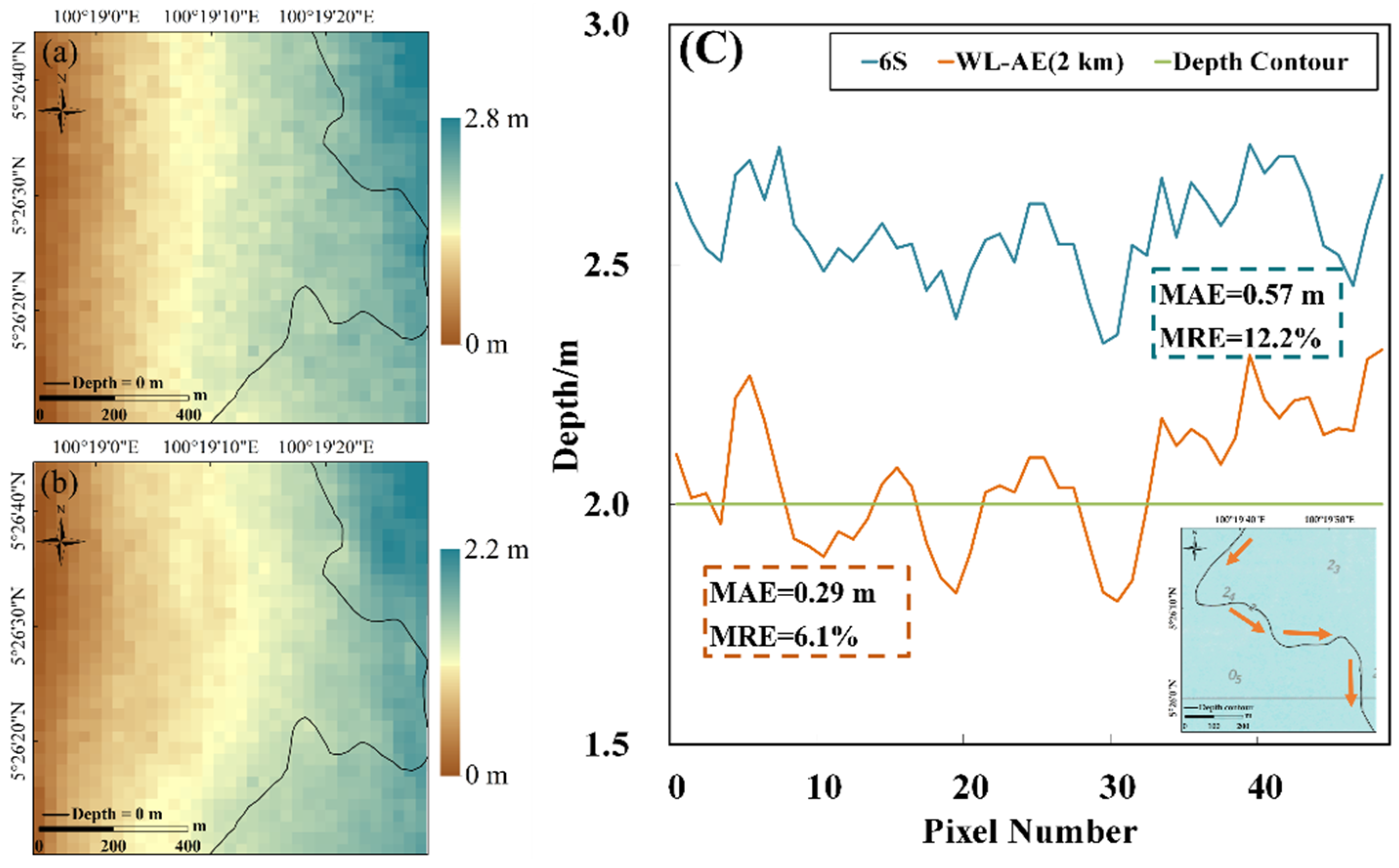
3.4.2. Assessment Analysis of the Segmental Inversion Accuracy

As seen in

Table 4. Accuracy of the Segmental Bathymetric Inversion Results in Penang and Socotra (interval: 5 m).

Study Area	Depth/m	0–5		5–10		10–15		15–20
	Model	MAE/m	MRE/%	MAE/m	MRE/%	MAE/m	MRE/%	MAE/m	MRE/%
Penang	6S	0.82	35.8	1.08	16.0	1.18	10.0	1.27	7.4
	WL-AE (1 km)	0.85	37.7	1.09	16.1	1.19	9.6	1.14	6.6
	WL-AE (1.5 km)	0.82	36.0	1.05	15.6	1.08	9.0	1.10	6.4
	WL-AE (2 km)	0.93	32.4	1.04	15.4	1.05	8.8	1.02	5.9
	WL-AE (3 km)	0.82	35.7	1.06	15.7	1.01	8.4	1.02	6.0
Socotra	6S	0.91	36.8	0.36	4.4	0.62	5.4	0.91	5.5
	WL-AE (1 km)	0.91	36.8	0.34	4.3	0.62	5.5	0.92	5.5
	WL-AE (1.5 km)	0.90	36.3	0.34	4.4	0.63	5.5	0.90	5.4
	WL-AE (2 km)	0.89	35.7	0.34	4.4	0.62	5.5	0.89	5.4
	WL-AE (3 km)	0.86	34.3	0.35	4.4	0.62	5.5	0.88	5.3

, WL-AE can improve the accuracy of the inversion results to a certain extent. However, affected by water depth, the accuracy changes differently in different segments. In Penang, the inversion results corresponding to WL-AE and 6S are significantly different in the 0–5 m depth section, and the MRE decreases first and then increases with increasing $R_{ns}$. When $R_{ns}$ = 2 km, the MRE = 32.4%, which is 3.4% lower than that of 6S. To further judge the effect of WL-AE on the water depth within 5 m, the depth section is divided again, and the accuracy of the inversion results at 0–4 m is calculated. The MAE and MRE of the bathymetric inversion results obtained under 6S and WL-AE are 0.76 m/41.9% and 0.68 m/31.4%, respectively, and the difference between the two MREs is 10.5%. The results show that WL-AE can effectively remove the influence of land on nearshore water pixels in this depth range, thus improving the accuracy of the inversion results. In the 5–20 m depth section, WL-AE has a certain effect on improving the accuracy of the inversion results, but this effect is relatively weak. The maximum MRE decreases in each depth section are 0.6%, 1.6%, and 1.5%, concentrated at $R_{ns}$ = 2 km and 3 km.

The inversion results of the two AC models are good at each depth section of Socotra. The maximum MRE for the 5–20 m depth is 5.5%, and the MAE is less than 1.0 m. In the 10–20 m depth section, the inversion accuracies of the different correction models are concentrated within 5.4% ± 0.1%, without significant fluctuations. As with Penang, the most obvious change in accuracy is in the 0–5 m depth section, the inversion accuracy improves from $R_{ns}$ = 1.5 km, and the MRE decreases by 0.5%, 1.1%, and 2.5% with increasing $R_{ns}$. In the 5–20 m depth section, the effect of WL-AE on improving the inversion accuracy is small, and the largest change occurs at $R_{ns}$ = 3 km. In the 15–20 m depth section, MAE and MRE corresponding to WL-AE are 0.88 m and 5.3%, respectively, which decrease by 0.03 m and 0.2% compared with those of 6S.

3.4.3. Influence Analysis of WL-AE Regarding Shallow Water Depth Inversion

Two sample areas were selected within 5 m water depth in Penang to explore the effects of 6S and WL-AE ($R_{ns}$ = 2 km) on bathymetric inversions, as shown in Figure 8. Figure 9a shows that the result obtained under 6S are generally higher, and the corresponding result distribution of WL-AE is more consistent with depth contour. The overall trends of the inversion results obtained under the two AC models are similar, but the deviation of the inversion results under the 6S model is large. The inversion results under WL-AE are mainly concentrated near the 2-m line, which is slightly different from the isobathic line. The MAE and MRE of WL-AE are 0.29 m and 6.1%, which are decreased by 0.28 m and 6.1%, respectively, compared with those of 6S.

In summary, WL-AE has a significant effect on improving the accuracy of nearshore bathymetric inversion because the bathymetric inversion model is based on the RT model of the water-optical field to establish the analytical expression of radiance (or reflectance) relative to depth [33]. In coastal areas, the optical complexity of seawater adds to eventual perturbations from the bottom and nearby land [3]. The WL-AE model effectively removes the influence of surrounding pixels on the radiance (or reflectance) of the target pixel, increases the realism of the image element value, improves the weight of the information from the water bottom, and thus improves the accuracy of the inversion results.

4. Discussion

Currently, common AC models are MODTRAN (moderate-resolution transmission), FLAASH (fast line-of-sight atmospheric analysis of spectral hypercubes), ATCOR (atmospheric and topographic correction for satellite imagery), and 6S. The first three models only consider the influence of the spatial distance between the background pixels and the target pixelz on AE [12,13]. The weight function is expressed as a radial index or Gaussian function. The 6S model not only considers the spatial distance but also the optical thickness of molecules and aerosols and expresses the weight function as an environmental function; then, the real reflectance is used to carry out a convolution operation with the function [3,14,15]. However, in boundary areas containing features with large radiance (or reflectance) differences, especially at the water–land boundaries, this difference directly affects $L_w$, and its influence on the weight function is not considered in the four models above. The WL-AE model proposed in this paper not only considers the difference in radiance but also overcomes the non-termination problem caused by abnormally highlighted pixels in the calculation process and designs an adjustable $R_{ns}$ to realize the effective calculation of equivalent background reflectance. In addition, we find that the operating efficiency of the WL-AE model is similar to that of 6S (less than 1 min), which is only 2–3 times higher.

Accurate AOT is important to improve the precision of AC. The main acquisition methods include satellite aerosol products, measured aerosol data, and software estimation. Due to the complex spatiotemporal variation of aerosol, diverse product types, and sparse measured data, the software (Atmospheric correction for OLI “lite”, ACOLITE) estimation method is adopted in this paper to obtain AOT, and the error caused by the estimation method itself is not evaluated. Since the launch of Landsat-8 in early 2013, several studies addressing water quality in inland and coastal waters have been conducted. The results indicated the need for a tailored approach to retrieve the water reflectance from OLI [34,35,36]. The 6S model simulates the transmission process of sunlight in the atmosphere in detail and performs well in the study of water optical remote sensing [31,37,38,39], so this paper improves based on the 6S model. In this paper, AE is improved based on the traditional RT model, which applies to the scenes of land and coastal water. This paper only evaluates the effect of the model in quantitative remote sensing of the water column, but it is also applicable to the research of object classification.

The radiance at the sensor is made up of three components from the sensed water column: surface reflectance, water column reflectance, and bottom reflectance [40]. When a wave appears, the whole sunglint (disk) is divided into small glitters that cover some parts of the ocean’s surface. The stronger the wave, the greater this area, and the distribution of the sunglint depends directly on the degree of the waves [41]. The remote sensing image used in this paper has a flat sea surface, so the model does not consider the effect of sea surface waves. The seafloor topography and water turbidity affect the RT of light inside the water column causing changes in the leaving-water signal, but the main influence of the water column signal is the water depth [42]. The paper describes the relative changes in the radiance of the ambient pixels and the target pixels, and the $R_{ns}$ is small, and it is considered that within this range, the seafloor topography and water turbidity remain consistent and thus have less influence on the final AC results. The model proposed in this paper only considers the transmission of light on the water surface, and the WL-AE model that considers the underwater RT process and is applicable to the sunglint region needs further study.

5. Conclusions

In this paper, the WL-AE model was proposed based on the limitations of the current AC models for water–land boundaries with obvious radiance (or reflectance) differences. The AC comparison test shows that the trends of the reflectance histograms of 6S and WL-AE are consistent, and the latter broadens the distribution range of albedo and has a smoother trend. After performing WL-AE correction, the entropy and contrast of the given image are significantly improved. In the visible wavelength, AE is not only related to the wavelength but also affected by the ground object types and water components in the study area. The difference between the two AC results is mainly concentrated at the water–land boundary and is extremely obvious in the green band, where the maximum $M_{rc}$ reaches 14.2%. The $Mrc$ and $Sd$ of the NIR band both at the water–land boundaries and in the region with only water increase with $R_{ns}$; this is mainly because the NIR band has a better response when making water–land distinctions and the AE produced from land to water is gradually removed with the increase in $R_{ns}$. The range of the AE produced on land is limited to approximately 3 km offshore water; the influence on water depth is mainly concentrated in shallow water, i.e., at 0–5 m depths. The MRE at 0–4 m in Penang is 31.4%, which is 10.5% lower than that of the 6S model, and in the 5–20 m water depth sections, the MRE of the WL-AE model inversion results are 15.4%, 8.8% and 5.9%, which are slightly different from those of 6S and are decreases of 0.6%, 1.2%, and 1.5%, respectively.

References

1. Zheng, X.; Li, Z.-L.; Zhang, X.; Shang, G. Quantification of the adjacency effect on measurements in the thermal infrared region. IEEE Trans. Geosci. Remote Sens. 2019, 57, 321–331. [Google Scholar] [CrossRef]
2. Vermote, E.F.; Tanre, D.; Deuze, J.L.; Herman, M.; Morcette, J.J. Second simulation of the satellite signal in the solar spectrum, 6S: An overview. IEEE Trans. Geosci. Remote Sens. 1997, 35, 675–686. [Google Scholar] [CrossRef]
3. Bulgarelli, B.; Zibordi, G. On the detectability of adjacency effects in ocean color remote sensing of mid-latitude coastal environments by SeaWiFS, MODIS-A, MERIS, OLCI, OLI and MSI. Remote Sens. Environ. 2018, 209, 423–438. [Google Scholar] [CrossRef] [PubMed]
4. Bulgarelli, B.; Kiselev, V.; Zibordi, G. Simulation and analysis of adjacency effects in coastal waters: A case study. Appl. Opt. 2014, 53, 1523. [Google Scholar] [CrossRef] [PubMed]
5. Lyzenga, D.R. Passive remote sensing techniques for mapping water depth and bottom features. Appl. Opt. 1978, 17, 379. [Google Scholar] [CrossRef] [PubMed]
6. Lyzenga, D.R. Shallow-water bathymetry using combined lidar and passive multispectral scanner data. Int. J. Remote Sens. 1985, 6, 115–125. [Google Scholar] [CrossRef]
7. Lyzenga, D.R.; Malinas, N.P.; Tanis, F.J. Multispectral bathymetry using a simple physically based algorithm. IEEE Trans. Geosci. Remote Sens. 2006, 44, 2251–2259. [Google Scholar] [CrossRef]
8. Putsay, M. A simple atmospheric correction method for the short wave satellite images. Int. J. Remote Sens. 1992, 13, 1549–1558. [Google Scholar] [CrossRef]
9. Sanders, L.C.; Schott, J.R.; Raqueño, R. A VNIR/SWIR atmospheric correction algorithm for hyperspectral imagery with adjacency effect. Remote Sens. Environ. 2001, 78, 252–263. [Google Scholar] [CrossRef]
10. Tanré, D.; Deschamps, P.Y.; Duhaut, P.; Herman, M. Adjacency effect produced by the atmospheric scattering in thematic mapper data. J. Geophys. Res. Atmos. 1987, 92, 12000. [Google Scholar] [CrossRef]
11. Guzzi, D.; Nardino, V.; Lastri, C.; Raimondi, V. A fast iterative procedure for adjacency effects correction on remote sensed data. Remote Sens. 2021, 13, 1799. [Google Scholar] [CrossRef]
12. Richter, R. A spatially adaptive fast atmospheric correction algorithm. Int. J. Remote Sens. 1996, 17, 1201–1214. [Google Scholar] [CrossRef]
13. Cooley, T.; Anderson, G.P.; Felde, G.W.; Hole, M.L.; Ratkowski, A.J.; Chetwynd, J.H.; Gardner, J.A.; Adlergolden, S.M.; Matthew, M.W.; Berk, A. FLAASH, a MODTRAN4-based atmospheric correction algorithm, its application and validation. In Proceedings of the IEEE International Geoscience and Remote Sensing Symposium, Toronto, ON, Canada, 24–28 June 2002; pp. 1414–1418. [Google Scholar] [CrossRef]
14. Minomura, M.; Kuze, H.; Takeuchi, N. Adjacency effect in the atmospheric correction of satellite remote sensing data: Evaluation of the influence of aerosol extinction profiles. Opt. Rev. 2001, 8, 133–141. [Google Scholar] [CrossRef]
15. Richter, R. A fast atmospheric correction algorithm applied to Landsat TM images. Int. J. Remote Sens. 1990, 11, 159–166. [Google Scholar] [CrossRef]
16. Kiselev, V.; Bulgarelli, B.; Heege, T. Sensor independent adjacency correction algorithm for coastal and inland water systems. Remote Sens. Environ. 2015, 157, 85–95. [Google Scholar] [CrossRef]
17. Bulgarelli, R.; Zibordi, G. Adjacency radiance around a small island: Implications for system vicarious calibrations. Appl. Opt. 2020, 59, C63–C69. [Google Scholar] [CrossRef] [PubMed]
18. Feng, L.; Hu, C. Land adjacency effects on MODIS aqua top-of-atmosphere radiance in the shortwave infrared: Statistical assessment and correction. J. Geophys. Res. Oceans 2017, 122, 4802–4818. [Google Scholar] [CrossRef]
19. Kaufman, Y.J.; Joseph, J.H. Determination of surface albedos and aerosol extinction characteristics from satellite imagery. J. Geophys. Res. Oceans 1982, 87, 1287. [Google Scholar] [CrossRef]
20. Schäfer, M.; Bierwirth, E.; Ehrlich, A.; Jäkel, E.; Wendisch, E. Airborne observations and simulations of three-dimensional radiative interactions between Arctic boundary layer clouds and ice floes. Atmos. Chem. Phys. 2015, 15, 8147–8163. [Google Scholar] [CrossRef] [Green Version]
21. Wang, T.; Du, L.; Yi, W.; Hong, J.; Zhang, L.; Zheng, J.; Li, C.; Ma, X.; Zhang, D.; Fang, W.; et al. An adaptive atmospheric correction algorithm for the effective adjacency effect correction of submeter-scale spatial resolution optical satellite images: Application to a WorldView-3 panchromatic image. Remote Sens. Environ. 2021, 259, 112412. [Google Scholar] [CrossRef]
22. Wright, L.A.; Kindel, B.C.; Pilewskie, P.; Leisso, N.P.; Kampe, T.U.; Schmidt, K.S. Below-cloud atmospheric correction of airborne hyperspectral imagery using simultaneous solar spectral irradiance observations. IEEE Trans. Geosci. Remote Sens. 2020, 59, 1392–1409. [Google Scholar] [CrossRef]
23. Harmel, T.; Chami, M.; Tormos, T.; Reynaud, N.; Danis, P.A. Sunglint correction of the multi-spectral instrument (msi)-sentinel-2 imagery over inland and sea waters from swir bands. Remote Sens. Environ. 2017, 204, 308–321. [Google Scholar] [CrossRef]
24. Bulgarelli, B.; Zibordi, G. Seasonal Impact of Adjacency Effects on Ocean Color Radiometry at the AAOT Validation Site. IEEE Geosci. Remote Sens. Lett. 2018, 15, 488–492. [Google Scholar] [CrossRef]
25. Ma, L.; Wang, N.; Liu, Y.; Zhao, Y.; Han, Q.; Wang, X.; Woolliams, E.R.; Bouvet, M.; Gao, C.; Li, C.; et al. An in-flight radiometric calibration method considering adjacency effects for high-resolution optical sensors over artificial targets. IEEE Trans. Geosci. Remote Sens. 2020, 60, 5600913. [Google Scholar] [CrossRef]
26. Duan, S.B.; Li, Z.L.; Gao, C.; Zhao, W.; Wu, H.; Qian, Y.; Leng, P.; Gao, M. Influence of adjacency effect on high-spatial-resolution thermal infrared imagery: Implication for radiative transfer simulation and land surface temperature retrieval. Remote Sens. Environ. 2020, 245, 111852. [Google Scholar] [CrossRef]
27. Yang, H.; Gordon, H.R.; Zhang, T. Island perturbation to the sky radiance over the ocean: Simulations. Appl. Opt. 1995, 34, 38354. [Google Scholar] [CrossRef]
28. Santer, R.; Schmechtig, C. Adjacency effects on water surfaces: Primary scattering approximation and sensitivity study. Appl. Opt. 2000, 39, 361. [Google Scholar] [CrossRef]
29. Ruddick, K.G.; Ovidio, F.; Rijkeboer, M. Atmospheric correction of SeaWiFS imagery for turbid coastal and inland waters. Appl. Opt. 2000, 39, 897–912. [Google Scholar] [CrossRef]
30. Sei, A. Analysis of adjacency effects for two Lambertian half-spaces. Int. J. Remote Sens. 2007, 28, 1873–1890. [Google Scholar] [CrossRef]
31. Zhang, H.; Ma, Y.; Zhang, J. Multi-dimensional analysis of atmospheric correction models on multi-spectral water depth inversion. Haiyang Xuebao 2022, 44, 145–160. [Google Scholar] [CrossRef]
32. Bulgarelli, B.; Zibordi, G.; Kiselev, V. Modeling the adjacency effects at AERONET-OC sites. Am. Inst. Phys. 2013, 1531, 943–946. [Google Scholar] [CrossRef]
33. Zhang, X.; Ma, Y.; Zhang, J. Shallow water bathymetry based on inherent optical properties using high spatial resolution multispectral imagery. Remote Sens. 2020, 12, 3027. [Google Scholar] [CrossRef]
34. Pahlevan, N.; Mangin, A.; Balasubramanian, S.V.; Smith, B.; Alikas, K.; Arai, K.; Barbosa, C.; Bélanger, S.; Binding, C.; Bresciani, M.; et al. ACIX-Aqua: A global assessment of atmospheric correction methods for Landsat-8 and Sentinel-2 over lakes, rivers, and coastal waters. Remote Sens. Environ. 2021, 258, 112366. [Google Scholar] [CrossRef]
35. Pahlevan, N.; Schott, J.R.; Franz, B.A.; Zibordi, G. Landsat 8 remote sensing reflectance (Rrs) products: Evaluations, intercomparisons, and enhancements. Remote Sens. Environ. 2017, 190, 289–301. [Google Scholar] [CrossRef]
36. Lymburner, L.; Botha, E.; Hestir, E.; Anstee, J.; Sagar, S.; Dekker, A.; Malthus, T. Landsat 8: Providing continuity and increased precision for measuring multi-decadal time series of total suspended matter. Remote Sens. Environ. 2016, 185, 108–118. [Google Scholar] [CrossRef]
37. López-Serrano, P.M.; Corral-Rivas, J.J.; Díaz-Varela, R.A.; Álvarez-González, J.G.; López-Sánchez, C.A. Evaluation of radiometric and atmospheric correction algorithms for aboveground forest biomass estimation using Landsat 5 TM data. Remote Sens. 2016, 8, 369. [Google Scholar] [CrossRef]
38. Nazeer, M.; Nichol, J.E.; Yung, Y.K. Evaluation of atmospheric correction models and Landsat surface reflectance product in an urban coastal environment. Int. J. Remote Sens. 2014, 35, 6271–6291. [Google Scholar] [CrossRef]
39. Hsu, H.J.; Huang, C.Y.; Jasinski, M.; Li, Y.; Gao, H.; Yamanokuchi, T.; Wang, C.G.; Chang, T.M.; Ren, H.; Kuo, C.Y.; et al. A semi-empirical scheme for bathymetric mapping in shallow water by ICESat-2 and Sentinel-2: A case study in the South China Sea. ISPRS J. Photogramm. Remote Sens. 2021, 178, 1–19. [Google Scholar] [CrossRef]
40. Zhang, Y.; Gao, J.; Yan, G.U. A simple method for mapping bathymetry over turbid coastal waters from MODIS data: Possibilities and limitations. Int. J. Remote Sens. 2011, 32, 7575–7590. [Google Scholar] [CrossRef]
41. Gardashov, R.H.; Eminov, M.S. Determination of sunglint location and its characteristics on observation from a METEOSAT 9 satellite. Int. J. Remote Sens. 2015, 36, 2584–2598. [Google Scholar] [CrossRef]
42. Lafon, V.; Froidefond, J.M.; Lahet, F.; Castaing, P. SPOT shallow water bathymetry of a moderately turbid tidal inlet based on field measurements. Remote Sens. Environ. 2002, 81, 136–148. [Google Scholar] [CrossRef]
Figure 1. Composition of the remote sensing signal of a water column. ① is the part that returns directly to the sensor through atmospheric action, that is, the atmospheric path radiation. ② is the portion of solar radiation reflected from surrounding features and entering the sensor by atmospheric action, that is, the solar radiation generated by the AE. ③ is the solar radiation entering the sensor reflected by the target.
Remotesensing 14 04769 g001
Figure 2. Flowchart of WL-AE.
Remotesensing 14 04769 g002
Figure 3. Image and depth point distributions. The control points and check points were randomly selected at a ratio of 2:1, and the points in each water depth section were as close as possible. (a) For Penang, there were a total of 266 depth points. (b) Socotra provided a total of 312 depth points. The Figure contains three ground tracks of ICESat-2, and the points are distributed along the track.
Remotesensing 14 04769 g003
Figure 4. Distribution of the CTS in the study area. To better show the boundary between water and land, Coastal imagery is used for display. (a) Penang, (b) Socotra; 1 is a mixed area of land and water (Mixed Zone), the ratio of water to land is 1:1, and 2 is the water-only area (Water Zone).
Remotesensing 14 04769 g004
Figure 5. Distribution of R r c by the band for Mixed Zone in Penang. (ad) are R n s   = 1 km, (eh) are R n s = 1.5 km, (il) are R n s = 2 km, and (mp) are R n s = 3 km. The differences between the two models in the blue, green, red, and NIR bands are shown.
Remotesensing 14 04769 g005
Figure 6. Distribution of R r c by the band for Mixed Zone in Socotra. (ad) are R n s = 1 km, (eh) are R n s = 1.5 km, (il) are R n s = 2 km, and (mp) are R n s = 3 km. The differences between the two models in the blue, green, red, and NIR bands are shown.
Remotesensing 14 04769 g006
Figure 7. Accuracy diagram of the bathymetric inversion results in the range of 20 m under the 6S and WL-AE correction results. (a) Penang; (b) Socotra.
Remotesensing 14 04769 g007
Figure 8. Sample bathymetric map of Penang. (a) shows the distribution of two sample areas in Penang; (b,c) show the sea charts of the sample areas. The large sample area corresponds to (b) and contains a 0-m depth contour; the small sample area corresponds to (c) and contains a 2-m depth contour.
Remotesensing 14 04769 g008
Figure 9. Bathymetric inversion results of Penang. (a) is the inversion result corresponding to 6S for the 0-m area; (b) is the inversion result corresponding to WL-AE for the 0 m area; (c) is the plot of the inversion results obtained at the 2 m isobaths, where the depth values on the isobaths are extracted in the direction shown by the arrow in the lower-right chart.
Remotesensing 14 04769 g009