
Evaluation of Satellite Images and Products for the Estimation of Regional Reference Crop Evapotranspiration in a Valley of the Ecuadorian Andes


Abstract
1. Introduction
2. Materials and Methods
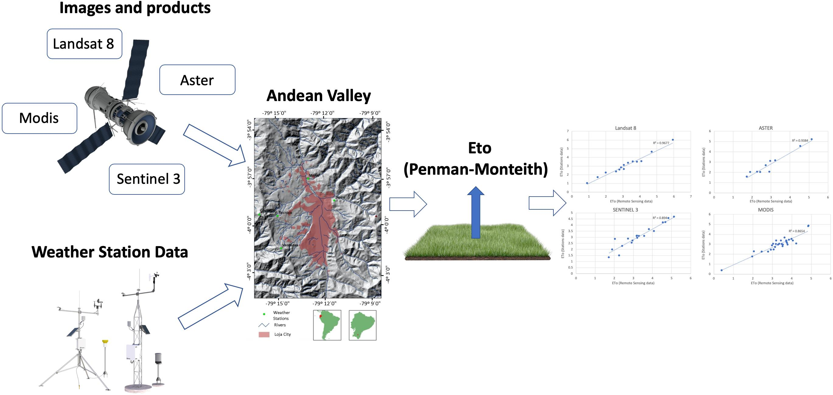
2.1. Study Area
2.2. The Penman–Monteith Equation
2.3. Information Collected
2.4. Calculation of ETo Using Meteorological Data
2.5. Calculation of ETo Using Remote Sensing Data
2.6. Product Evaluation
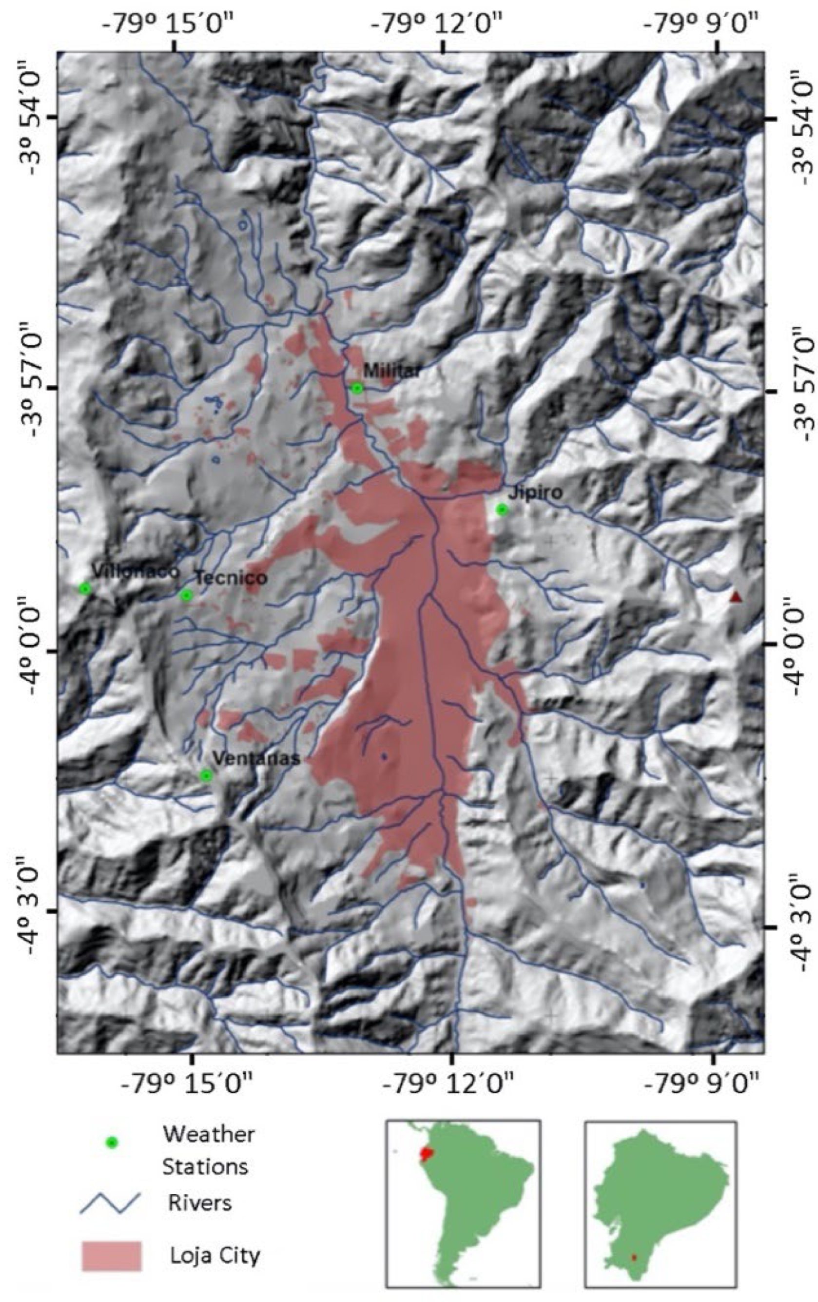
3. Results and Discussion
4. Conclusions
Author Contributions
Funding
Data Availability Statement
Conflicts of Interest
References
- Walker, E.; García, G.A.; Venturini, V. Estimación de la evapotranspiración real en zonas de llanura mediante productos de humedad de suelo de la misión SMAP. Rev. Teledetección 2018, 52, 17–26. [Google Scholar] [CrossRef]
- Sur, C.; Kang, S.; Kim, J.; Choi, M. Remote sensing-based evapotranspiration algorithm: A case study of all sky conditions on a regional scale. GISci. Remote Sens. 2015, 52, 627–642. [Google Scholar] [CrossRef]
- Marini, F.; Santamaría, M.; Oricchio, P.; Di Bella, C.M.; Basualdo, A. Estimación de evapotranspiración real (ETR) y de evapotranspiración potencial (ETP) en el sudoeste bonaerense (Argentina) a partir de imágenes MODIS. Rev. Teledetección 2017, 48, 29–41. [Google Scholar] [CrossRef][Green Version]
- Allen, R.; Pereira, L.; Raes, D.; Smith, M. Crop. Evapotranspiration: Guidelines for Computing Crop Water Requeriments; FAO Irrigation and Drainage Paper No. 56; Food and Agriculture Organization of the United Nations: Rome, Italy, 1998; p. 338. [Google Scholar]
- Sánchez, M.; Chuvieco, E. Estimación de la evapotranspiración del cultivo de referencia, ET0, a partir de imágenes NOAA-AVHRR. Rev. Teledetección 2000, 14, 11–21. [Google Scholar]
- Rivas, R.; Caselles, V. A simplified equation to estimate spatial reference evaporation from remote sensing-based surface temperature and local meteorological data. Remote Sens. Environ. 2004, 93, 68–76. [Google Scholar] [CrossRef]
- Sobrino, J.A.; Gómez, M.; Jiménez-Muñoz, J.C.; Olioso, A. Application of a simple algorithm to estimate daily evapotranspiration from NOAA–AVHRR images for the Iberian Peninsula. Remote Sens. Environ. 2007, 110, 139–148. [Google Scholar] [CrossRef]
- Tasumi, M.; Trezza, R.; Allen, R.G.; Wright, J.L. Satellite-Based Energy Balance for Mapping Evapotranspiration with Internalized Calibration (METRIC)-Applications. J. Irrig. Drain. Eng. 2008, 133, 395–406. [Google Scholar]
- Venturini, V.; Islam, S.; Rodríguez, L. Estimation of evaporative fraction and evapotranspiration from MODIS products using a complementary based model. Remote Sens. Environ. 2008, 112, 132–141. [Google Scholar] [CrossRef]
- Barraza, V.; Restrepo-Coupe, N.; Huete, A.; Grings, F.; Van Gorsel, E. Passive microwave and optical index approaches for estimating surface conductance and evapotranspiration in forest ecosystems. Agric. For. Meteorol. 2015, 213, 126–137. [Google Scholar] [CrossRef]
- Knipper, K.; Hogue, T.; Scott, R.; Franz, K. Evapotranspiration estimates derived using multi-platform remote sensing in a semiarid region. Remote Sens. 2017, 9, 184. [Google Scholar] [CrossRef]
- Anderson, M.C.; Norman, J.M.; Diak, G.R.; Kustas, W.P.; Mecikalski, J.R. A two-source time-integrated model for estimating surface fluxes using thermal infrared remote sensing. Remote Sens. Environ. 1997, 60, 195–216. [Google Scholar] [CrossRef]
- Bastiaanssen, W.G.M.; Menenti, M.; Feddes, R.A.; Holtslag, A.A.M. A remote sensing surface energy balance algorithm for land (SEBAL): 1. Formulation. J. Hydrol. 1998, 212, 198–212. [Google Scholar] [CrossRef]
- Allen, R.G.; Tasumi, M.; Trezza, R. Satellite-based energy balance for mapping evapotranspiration with internalized calibration (METRIC)-model. J. Irrig. Drain. Eng. 2007, 133, 380–394. [Google Scholar] [CrossRef]
- Sánchez, J.M.; Scavone, G.; Caselles, V.; Valor, E.; Copertino, V.A.; Telesca, V. Monitoring daily evapotranspiration at a regional scale from Landsat-TM and ETM+data: Application to the Basilicata region. J. Hydrol. 2008, 351, 58–70. [Google Scholar] [CrossRef]
- Jiang, L.; Islam, S. Estimation of surface evaporation map over southern Great Plains using remote sensing data. Water Resour. Res. 2001, 37, 329–340. [Google Scholar] [CrossRef]
- Nishida, K.; Nemani, R.R.; Glassy, J.M.; Running, S.W. Development of an evapotranspiration index from aqua/MODIS for monitoring surface moisture status. IEEE Trans. Geosci. Remote Sens. 2003, 41, 493–501. [Google Scholar] [CrossRef]
- Tang, Q.H.; Peterson, S.; Cuenca, R.H.; Hagimoto, Y.; Lettenmaier, D.P. Satellite-based near- real-time estimation of irrigated crop water consumption. J. Geophys. Res. Atmos. 2009, 114, D05114. [Google Scholar] [CrossRef]
- Castañeda-Ibáñez, C.; Martínez-Menes, M.; Pascual-Ramírez, F.; Flores-Magdaleno, H.; Fernández-Reynoso, D.; Esparza-Govea, S. Estimación de coeficientes de cultivo mediante sensores remotos en el distrito de riego río Yaqui, Sonora, México. Agrociencia 2015, 49, 221–232. [Google Scholar]
- Mu, Q.; Heinsch, F.A.; Zhao, M.; Running, S.W. Development of a global evapotranspiration algorithm based on MODIS and global meteorology data. Remote Sens. Environ. 2007, 111, 519–536. [Google Scholar] [CrossRef]
- Mu, Q.Z.; Zhao, M.S.; Running, S.W. Improvements to a MODIS global terrestrial evapotranspiration algorithm. Remote Sens. Environ. 2011, 115, 1781–1800. [Google Scholar] [CrossRef]
- Zhang, K.; Kimball, J.S.; Mu, Q.; Jones, L.A.; Goetz, S.J.; Running, S.W. Satellite based analysis of northern ET trends and associated changes in the regional water balance from 1983 to 2005. J. Hydrol. 2009, 379, 92–110. [Google Scholar] [CrossRef]
- Fisher, J.B.; Tu, K.P.; Baldocchi, D.D. Global estimates of the land-atmosphere water flux based on monthly AVHRR and ISLSCP-II data, validated at 16 FLUX- NET sites. Remote Sens. Environ. 2008, 112, 901–919. [Google Scholar] [CrossRef]
- Miralles, D.G.; Holmes, T.R.H.; De Jeu, R.A.M.; Gash, J.H.; Meesters, A.G.C.A.; Dolman, A.J. Global land-surface evaporation estimated from satellite- based observations. Hydrol. Earth Syst. Sci. 2011, 15, 453–469. [Google Scholar] [CrossRef]
- Wang, K.C.; Wang, P.; Li, Z.Q.; Cribb, M.; Sparrow, M. A simple method to estimate actual evapotranspiration from a combination of net radiation, vegetation index, and temperature. J. Geophys. Res. Atmos. 2007, 112, D15107. [Google Scholar] [CrossRef]
- Zeng, Z.Z.; Piao, S.L.; Lin, X.; Yin, G.D.; Peng, S.S.; Ciais, P.; Myneni, R.B. Global evapotranspiration over the past three decades: Estimation based on the water balance equation combined with empirical models. Environ. Res. Lett. 2012, 7, 014026. [Google Scholar] [CrossRef]
- Long, D.; Longuevergne, L.; Scanlon, B.R. Uncertainty in evapotranspiration from land surface modeling, remote sensing, and GRACE satellites. Water Resour. Res. 2014, 50, 1131–1151. [Google Scholar] [CrossRef]
- Kumar, U.; Rashmi; Chatterjee, C.; Raghuwanshi, N.S. Comparative Evaluation of Simplified Surface Energy Balance Index-Based Actual ET against Lysimeter Data in a Tropical River Basin. Sustainability 2021, 13, 13786. [Google Scholar] [CrossRef]
- Oñate-Valdivieso, F.; Oñate-Paladines, A.; Collaguazo, M. Spatiotemporal Dynamics of Soil Impermeability and Its Impact on the Hydrology of An Urban Basin. Land 2022, 11, 250. [Google Scholar] [CrossRef]
- Oñate-Valdivieso, F.; Fries, A.; Mendoza, K.; Gonzalez-Jaramillo, V.; Pucha-Cofrep, F.; Rollenbeck, R.; Bendix, J. Temporal and spatial analysis of precipitation patterns in an Andean region of southern Ecuador using LAWR weather radar. Meteorol. Atmos. Phys. 2018, 130, 473–484. [Google Scholar] [CrossRef]
- U.S. Geological Survey (USGS). Earthexplorer. Available online: https://earthexplorer.usgs.gov (accessed on 18 November 2021).
- Copernicus Open Access Hub. Available online: https://scihub.copernicus.eu/dhus/#/home (accessed on 5 December 2021).
- Richter, R.; Schläpfer, D. Atmospheric/Topographic Correction for Satellite Imagery: ATCOR-2/3 User Guide, DLR-IB 565-01/15; German Aerospace Center: Wessling, Germany, 2015. [Google Scholar]
- Jensen, M.E.; Burmann, R.D.; Allen, R.G. Evaporation and Irrigation Water Requirements. In ASCE Manual and Reports on Engineering Practice; American Society of Civil Engineers: New York, NY, USA, 2016; Volume 70, p. 360. [Google Scholar]
- Li, Y.Y.; Liu, Y.; Ranagalage, M.; Zhang, H.; Zhou, R. Examining land use/land cover change and the summertime surface urban heat island effect in fast-growing greater hefei, China: Implications for sustainable land development. ISPRS Int. J. Geo-Inf. 2020, 9, 568. [Google Scholar] [CrossRef]
- Valor, E.; Caselles, V. Mapping land surface emissivity from NDVI: Application to European, African, and South American areas. Remote Sens. Environ. 1996, 57, 167–184. [Google Scholar] [CrossRef]
- Meng, X.; Cheng, J.; Zhao, S.; Liu, S.; Yao, Y. Estimating Land Surface Temperature from Landsat-8 Data using the NOAA JPSS Enterprise Algorithm. Remote Sens. 2019, 11, 155. [Google Scholar] [CrossRef]
- Ninyerola, M.; Pons, X.; Roure, J.M. A methodological approach of climatological modelling of air temperature and precipitation. Int. J. Climatol. 2000, 20, 1823–1841. [Google Scholar] [CrossRef]
- Carmona, F.; Rivas, R.; Kruse, E. Estimating daily net radiation in the FAO Penman-Monteith method. Theor. Appl. Climatol. 2017, 129, 89–95. [Google Scholar] [CrossRef]
- Bastiaanssen, W.G. SEBAL-based sensible and latent heat fluxes in the irrigated Gediz Basin, Turkey. J. Hydrol. 2000, 229, 87–100. [Google Scholar] [CrossRef]
- Oñate-Valdivieso, F.; Uchuari, V.; Oñate-Paladines, A. Large-Scale Climate Variability Patterns and Drought: A Case of Study in South—America. Water Resour. Manag. 2020, 34, 2061–2079. [Google Scholar] [CrossRef]
- Karavitis, C.A.; Alexandris, S.G.; Tsesmelis, D.E.; Athanasopoulos, G. Application of the Standardized Precipitation Index (SPI) in Greece. Water 2011, 3, 787–805. [Google Scholar] [CrossRef]
- Goovaerts, P. Geostatistical approaches for incorporating elevation into the spatial interpolation of rainfall. J. Hydrol. 2000, 228, 113–129. [Google Scholar] [CrossRef]


| Resolution | Satellite Data | |||
|---|---|---|---|---|
| LANDSAT 8 | SENTINEL 3 | ASTER | MODIS. | |
| Radiometric (bits) | 16 | - | 8–16 | 12 |
| Spatial (m) | 30 (Coastal/Aerosol) 30 (B,G,R,NIR,SWIR) 100 (TIR) | 500 (S1-S60) 1000 (S7-S9) | 15 (VNIR) 30 (SWIR) 90 (TIR) | 250 (B1-2) 500(B3-7) 1000 (B8-36) |
| Spectral (bands) | 11 | 11 (SLSTR) 21 (OLCI) | 14 | 36 |
| Temporal (days) | 16 | 2 (SLSTR) 1 (OLCI) | 16 | 1 |
| Acquisition dates | 7 January 2017 19 August 2017 20 September 2017 | 7 May 2017 24 June 2017 14 July 2017 20 September 2017 | 7 May 2017 24 June 2017 | 17 January 2017 13 February 2017 29 March 17 14 July 2017 14 August 2017 19 September 2017 |
| Station | Longitude | Latitude | Elevation (masl) |
|---|---|---|---|
| Militar | 79°13′03.1″W | 03°56′52.6″S | 2033 |
| Jipiro | 79°11′23.5″W | 03°58′15.7″S | 2218 |
| Tecnico | 79°14′59.6″W | 03°59′14.9″S | 2377 |
| Ventanas | 79°14′46.0″W | 04°01′18.9″S | 2816 |
| Villonaco | 79°16′09.9″W | 03°59′10.6″S | 2952 |
| Date | Sensor | Equation to Calculate Ta (°C) |
|---|---|---|
| 7 January 2017 | LANDSAT 8 | Ta = 31.901 − 0.00786z + 0.0893Ts |
| 17 January 2017 | MODIS | Ta = 79.961 − 0.01546z − 1.1131Ts |
| 13 February 2017 | MODIS | Ta = 27.239 − 0.00675z + 0.1313Ts |
| 29 March 2017 | MODIS | Ta = 38.777 − 0.008317z − 0.133Ts |
| 7 May 2017 | ASTER | Ta = 28.963 − 0.00585z + 0.01104Ts |
| SENTINEL 3 | Ta = 34.6518 − 0.00733z − 0.1604Ts | |
| 24 June 2017 | ASTER | Ta = 28.991 − 0.00663z + 0.05198Ts |
| SENTINEL 3 | Ta = 21.7586 − 0.00625z + 0.3755Ts | |
| 14 July 2017 | SENTINEL 3 | Ta = 31.7595 − 0.00771z + 0.0356Ts |
| MODIS | Ta = 30.696 − 0.00723z + 0.0220Ts | |
| 14 August 2017 | MODIS | Ta = 40.953 − 0.00875z − 0.2319Ts |
| 19 August 2017 | LANDSAT 8 | Ta = 25.822 − 0.00414z − 0.0000201Ts |
| 19 September 2017 | MODIS | Ta = 8.785 − 0.004197z − 0.5991Ts |
| 20 September 2017 | LANDSAT 8 | Ta = 34.122 − 0.00837z + 0.0667Ts |
| SENTINEL 3 | Ta = 31.288 − 0.00783z + 0.1384Ts |
| Date | Militar | Jipiro | Tecnico | Ventanas | Villonaco |
|---|---|---|---|---|---|
| 7 January 2017 | 2.80 | 1.52 | 2.00 | 0.90 | 5.94 |
| 17 January 2017 | 3.54 | 3.77 | 4.23 | 0.40 | 3.15 |
| 13 February 2017 | 3.86 | 3.72 | 3.08 | 4.07 | 3.55 |
| 29 March 2017 | 2.46 | 3.00 | 2.94 | 1.98 | 3.05 |
| 7 May 2017 | 1.91 | 2.28 | 2.93 | 1.74 | 4.56 |
| 24 June 2017 | 2.74 | 3.23 | 2.44 | 2.97 | 5.15 |
| 14 July 2017 | 2.06 | 3.21 | 3.31 | 3.20 | 4.86 |
| 14 August 2017 | 3.45 | 3.63 | 3.49 | 3.36 | 4.85 |
| 19 August 2017 | 2.61 | 2.90 | 3.07 | 3.31 | 3.07 |
| 19 September 2017 | 3.73 | 4.00 | 3.79 | 2.80 | 2.75 |
| 20 September 2017 | 3.84 | 4.70 | 4.09 | 3.59 | 3.43 |
| Date | Sensor | Militar | Jipiro | Tecnico | Ventanas | Villonaco |
|---|---|---|---|---|---|---|
| 7 January 2017 | LANDSAT | 2.56 | 1.67 | 2.20 | 1.00 | 5.99 |
| 17 January 2017 | MODIS | 2.78 | 3.11 | 3.06 | 0.37 | 2.70 |
| 13 February 2017 | MODIS | 3.45 | 3.37 | 2.47 | 3.37 | 2.96 |
| 29 March 2017 | MODIS | 2.25 | 2.88 | 2.44 | 1.75 | 3.05 |
| 7 May 2017 | ASTER | 2.01 | 2.02 | 2.04 | 1.56 | 4.53 |
| SENTINEL 3 | 1.99 | 1.50 | 2.54 | 1.35 | 4.21 | |
| 24 June 2017 | ASTER | 2.65 | 3.15 | 2.00 | 3.09 | 5.19 |
| SENTINEL 3 | 2.87 | 2.95 | 2.28 | 2.73 | 4.68 | |
| 14 July 2017 | SENTINEL 3 | 2.85 | 3.12 | 3.11 | 3.09 | 4.56 |
| MODIS | 2.27 | 3.35 | 2.96 | 3.01 | 4.86 | |
| 14 August 2017 | MODIS | 3.37 | 3.65 | 3.01 | 3.03 | 4.80 |
| 19 August 2017 | LANDSAT | 2.33 | 2.80 | 2.63 | 3.32 | 3.08 |
| 19 September 2017 | MODIS | 3.24 | 3.53 | 2.95 | 2.26 | 2.75 |
| 20 September 2017 | LANDSAT | 3.46 | 4.61 | 3.52 | 3.49 | 3.57 |
| SENTINEL 3 | 3.65 | 4.23 | 3.50 | 3.10 | 3.43 |
| Date | Sensor | Militar | Jipiro | Tecnico | Ventanas | Villonaco | AVG | STD |
|---|---|---|---|---|---|---|---|---|
| 7 January 2017 | LANDSAT 8 | 0.24 | 0.15 | 0.20 | 0.10 | 0.05 | 0.15 | 0.08 |
| 17 January 2017 | MODIS | 0.76 | 0.66 | 1.17 | 0.03 | 0.45 | 0.61 | 0.42 |
| 13 February 2017 | MODIS | 0.41 | 0.35 | 0.61 | 0.70 | 0.59 | 0.53 | 0.15 |
| 29 March 2017 | MODIS | 0.21 | 0.12 | 0.50 | 0.23 | 0.00 | 0.21 | 0.18 |
| 7 May 2017 | ASTER | 0.10 | 0.26 | 0.89 | 0.18 | 0.03 | 0.29 | 0.35 |
| SENTINEL 3 | 0.08 | 0.78 | 0.39 | 0.39 | 0.35 | 0.40 | 0.25 | |
| 24 June 2017 | ASTER | 0.09 | 0.08 | 0.44 | 0.12 | 0.04 | 0.15 | 0.16 |
| SENTINEL 3 | 0.13 | 0.28 | 0.16 | 0.24 | 0.47 | 0.26 | 0.13 | |
| 14 July 2017 | SENTINEL 3 | 0.79 | 0.09 | 0.20 | 0.11 | 0.30 | 0.30 | 0.29 |
| MODIS | 0.21 | 0.14 | 0.35 | 0.19 | 0.00 | 0.18 | 0.13 | |
| 14 August 2017 | MODIS | 0.08 | 0.02 | 0.48 | 0.33 | 0.05 | 0.19 | 0.20 |
| 19 August 2017 | LANDSAT 8 | 0.28 | 0.10 | 0.44 | 0.01 | 0.01 | 0.17 | 0.19 |
| 19 September 2017 | MODIS | 0.49 | 0.47 | 0.84 | 0.54 | - | 0.59 | 0.17 |
| 20 September 2017 | LANDSAT 8 | 0.38 | 0.09 | 0.57 | 0.10 | - | 0.29 | 0.23 |
| SENTINEL 3 | 0.19 | 0.47 | 0.59 | 0.49 | - | 0.44 | 0.17 | |
| AVG | 0.30 | 0.27 | 0.52 | 0.25 | 0.20 | |||
| STD | 0.23 | 0.05 | 0.08 | 0.04 | 0.05 |
| Sensor | Parameter | Militar | Jipiro | Tecnico | Ventanas | Villonaco |
|---|---|---|---|---|---|---|
| LANDSAT 8 | Average | 0.30 | 0.11 | 0.40 | 0.07 | 0.02 |
| STD | 0.07 | 0.03 | 0.19 | 0.05 | 0.03 | |
| ASTER | Average | 0.10 | 0.17 | 0.67 | 0.15 | 0.03 |
| STD | 0.01 | 0.13 | 0.32 | 0.04 | 0.01 | |
| SENTINEL 3 | Average | 0.30 | 0.41 | 0.34 | 0.31 | 0.28 |
| STD | 0.33 | 0.29 | 0.20 | 0.17 | 0.09 | |
| MODIS | Average | 0.36 | 0.29 | 0.66 | 0.34 | 0.18 |
| STD | 0.25 | 0.24 | 0.30 | 0.25 | 0.28 |
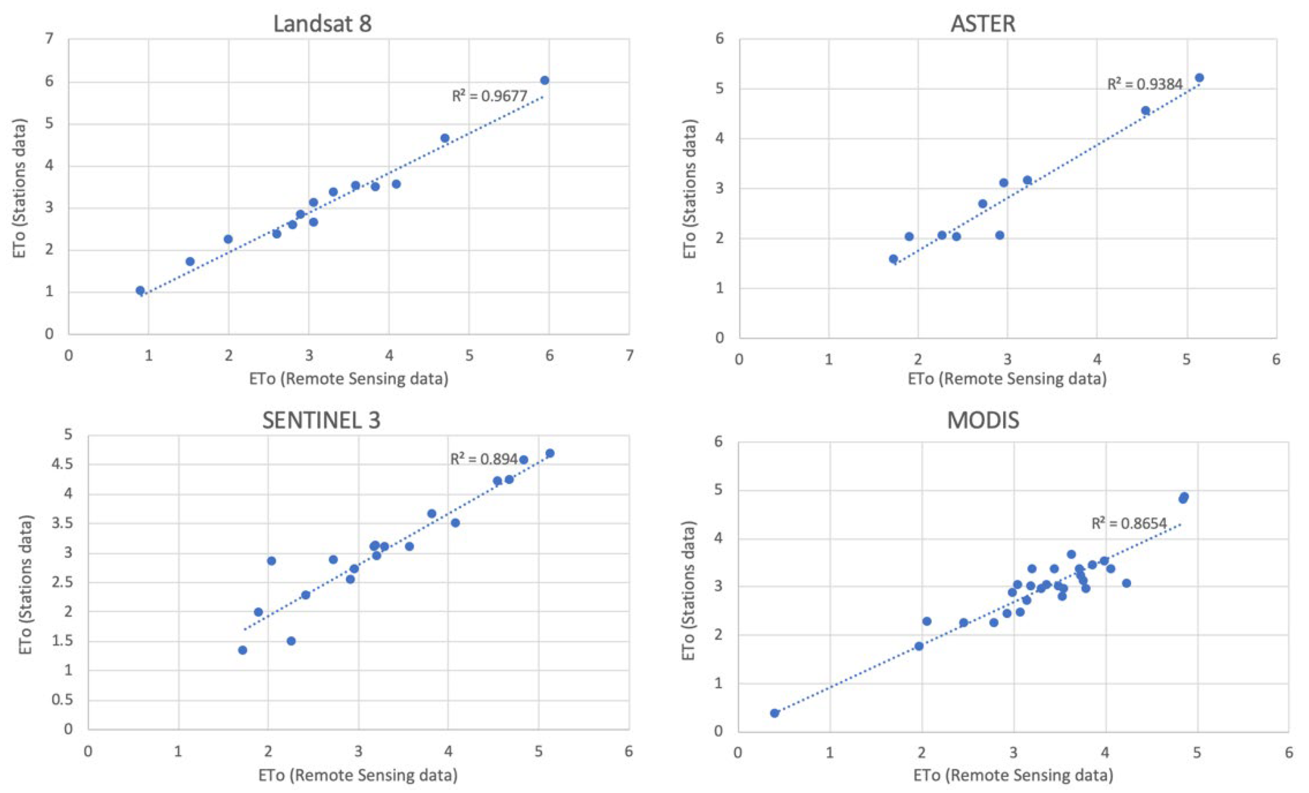
| Sensor | NSE | R2 | RMSE |
|---|---|---|---|
| LANDSAT 8 | 0.994 | 0.968 | 0.060 |
| ASTER | 0.988 | 0.938 | 0.067 |
| SENTINEL 3 | 0.985 | 0.894 | 0.110 |
| MODIS | 0.979 | 0.865 | 0.160 |
Publisher’s Note: MDPI stays neutral with regard to jurisdictional claims in published maps and institutional affiliations. |
© 2022 by the authors. Licensee MDPI, Basel, Switzerland. This article is an open access article distributed under the terms and conditions of the Creative Commons Attribution (CC BY) license (https://creativecommons.org/licenses/by/4.0/).
Share and Cite
Oñate-Valdivieso, F.; Oñate-Paladines, A.; Núñez, D. Evaluation of Satellite Images and Products for the Estimation of Regional Reference Crop Evapotranspiration in a Valley of the Ecuadorian Andes. Remote Sens. 2022, 14, 4630. https://doi.org/10.3390/rs14184630
Oñate-Valdivieso F, Oñate-Paladines A, Núñez D. Evaluation of Satellite Images and Products for the Estimation of Regional Reference Crop Evapotranspiration in a Valley of the Ecuadorian Andes. Remote Sensing. 2022; 14(18):4630. https://doi.org/10.3390/rs14184630
Chicago/Turabian StyleOñate-Valdivieso, Fernando, Arianna Oñate-Paladines, and Deiber Núñez. 2022. "Evaluation of Satellite Images and Products for the Estimation of Regional Reference Crop Evapotranspiration in a Valley of the Ecuadorian Andes" Remote Sensing 14, no. 18: 4630. https://doi.org/10.3390/rs14184630
APA StyleOñate-Valdivieso, F., Oñate-Paladines, A., & Núñez, D. (2022). Evaluation of Satellite Images and Products for the Estimation of Regional Reference Crop Evapotranspiration in a Valley of the Ecuadorian Andes. Remote Sensing, 14(18), 4630. https://doi.org/10.3390/rs14184630