

Airborne Coherent GNSS Reflectometry and Zenith Total Delay Estimation over Coastal Waters


Abstract
:1. Introduction
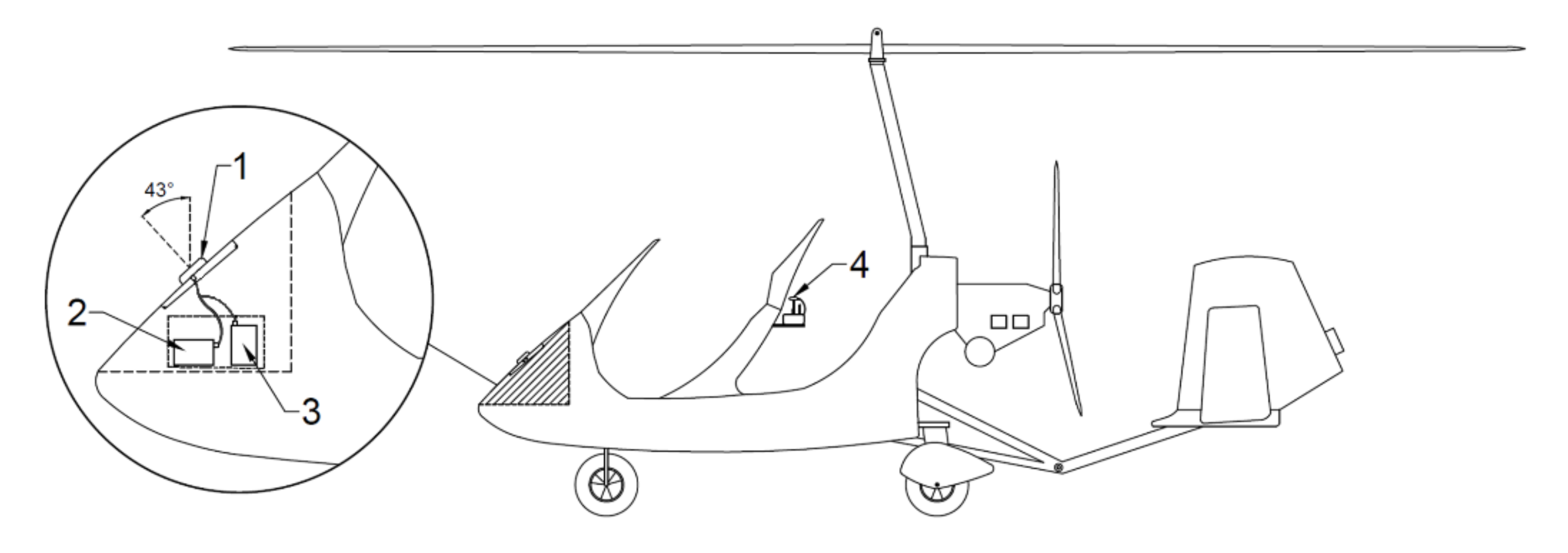
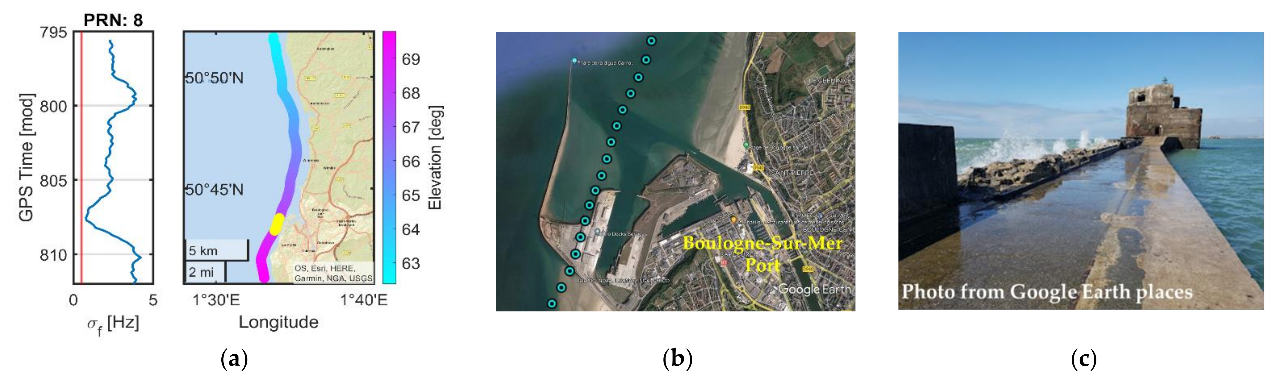
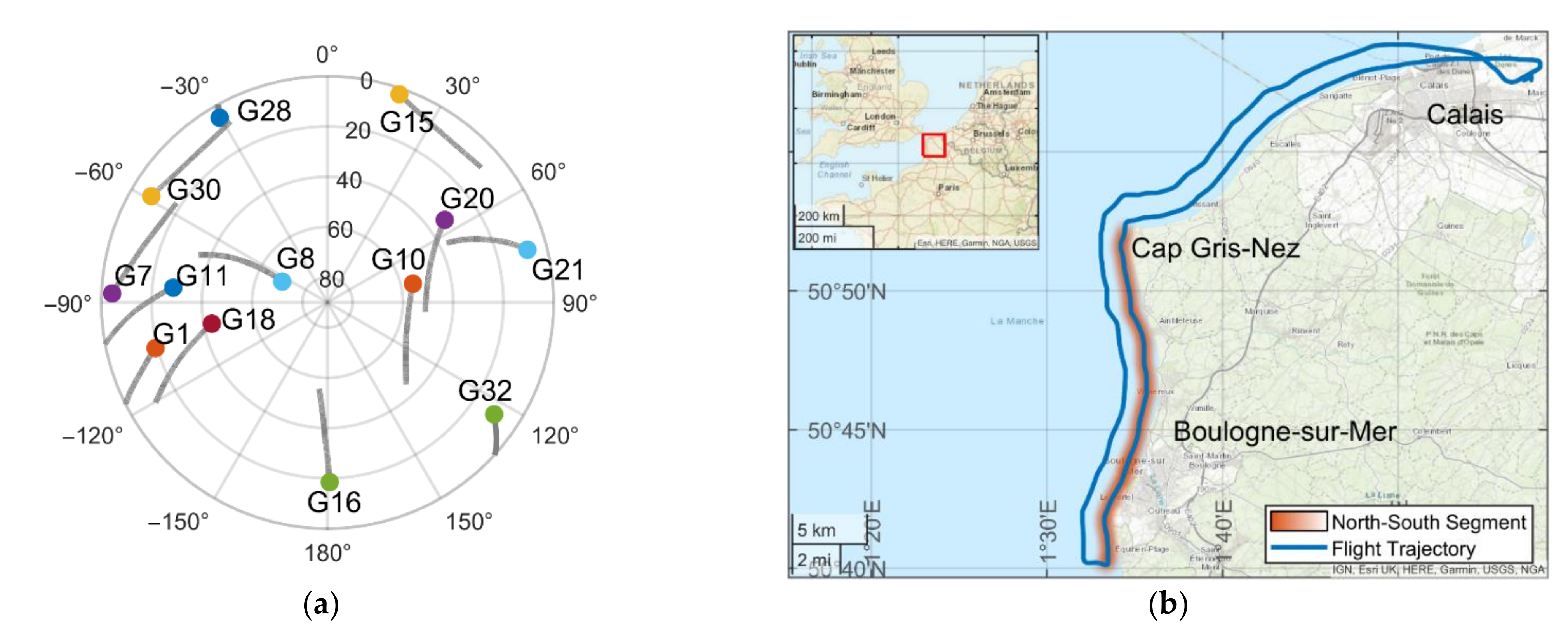
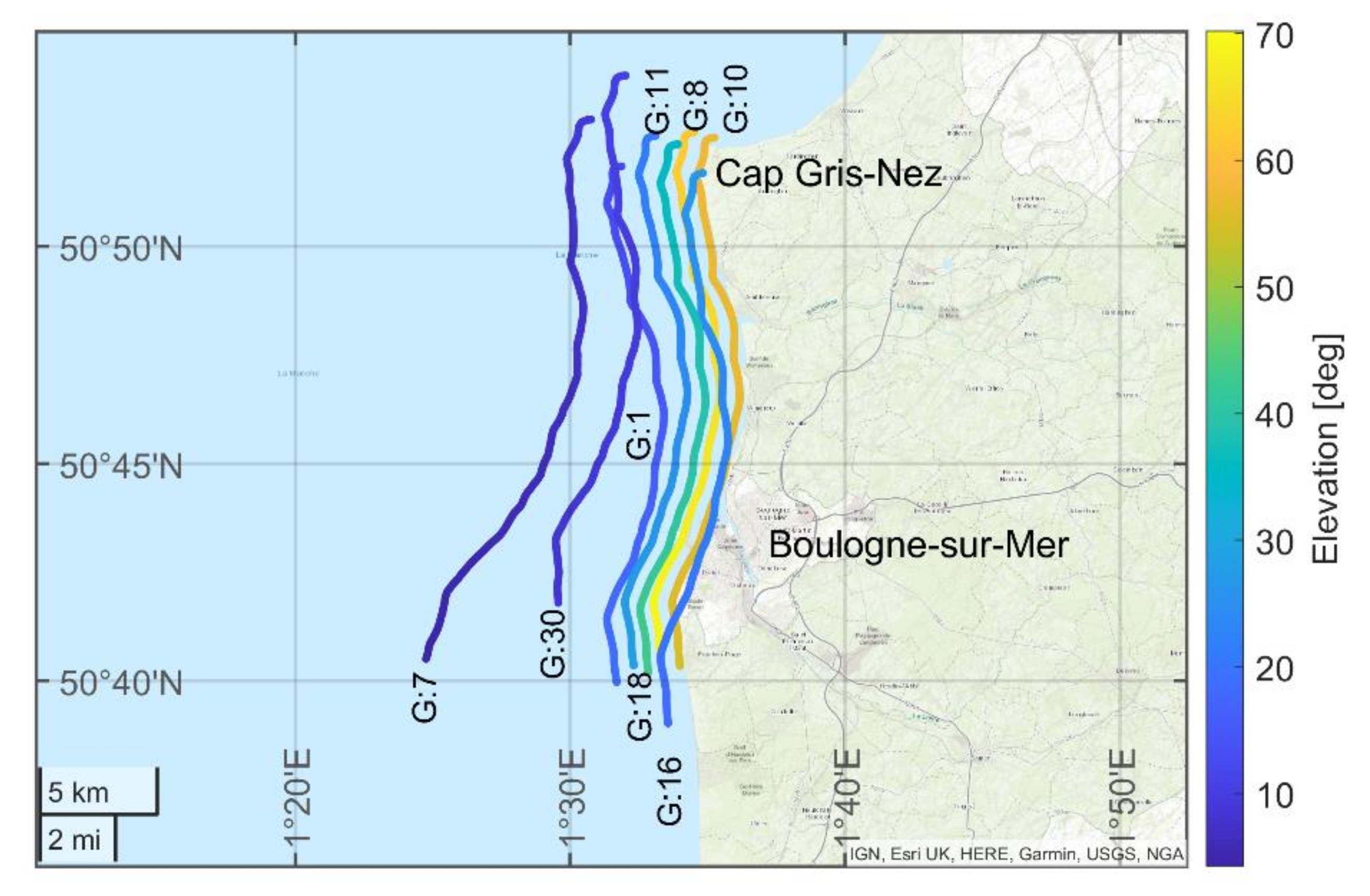
2. Experiment
3. GNSS-R Data and Methods
3.1. Data and Processing
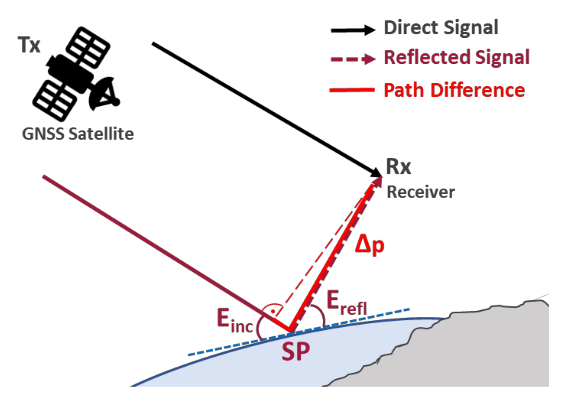
3.1.1. Geometrical Path Difference Model
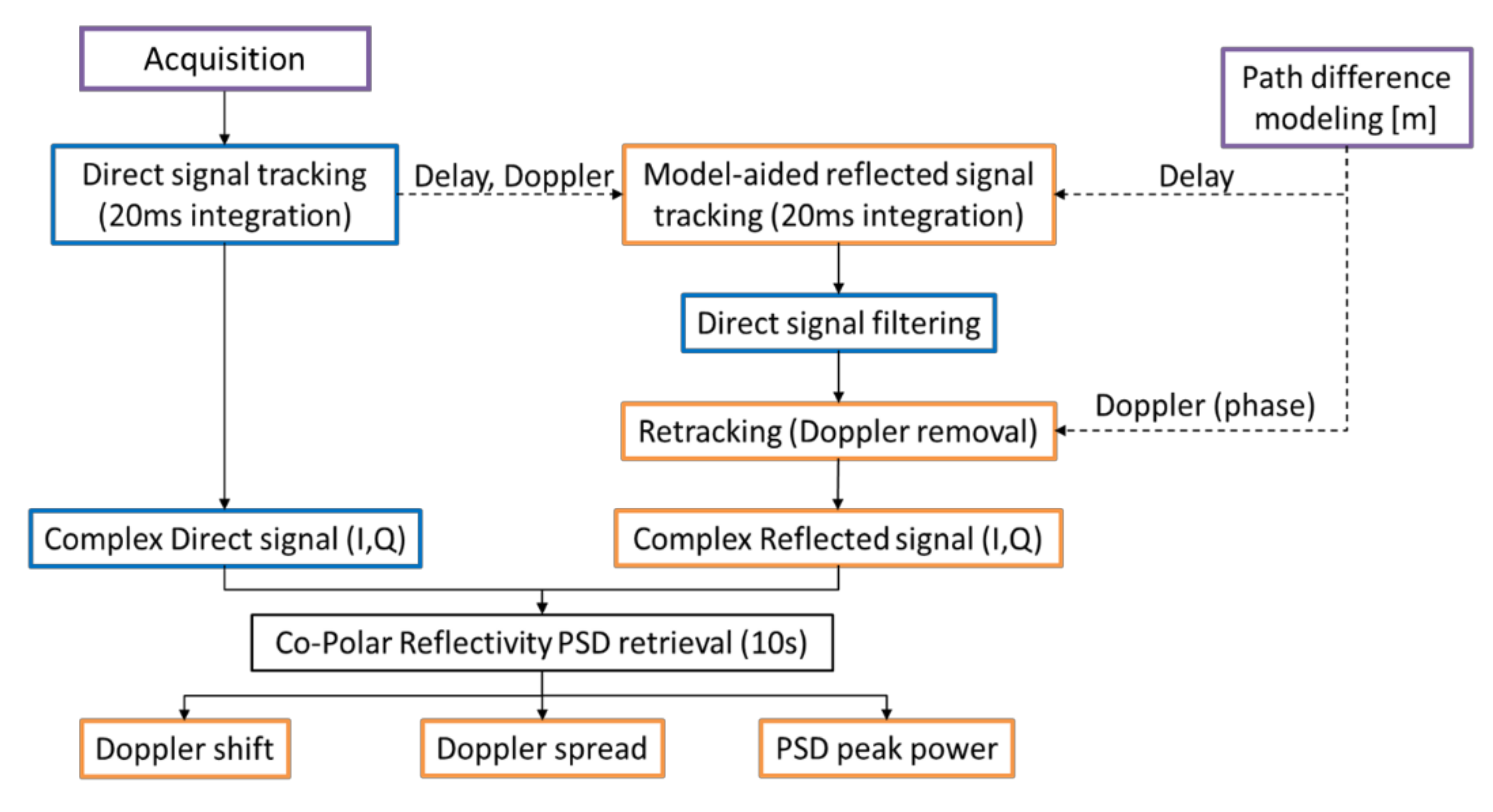
3.1.2. Tracking and Retracking
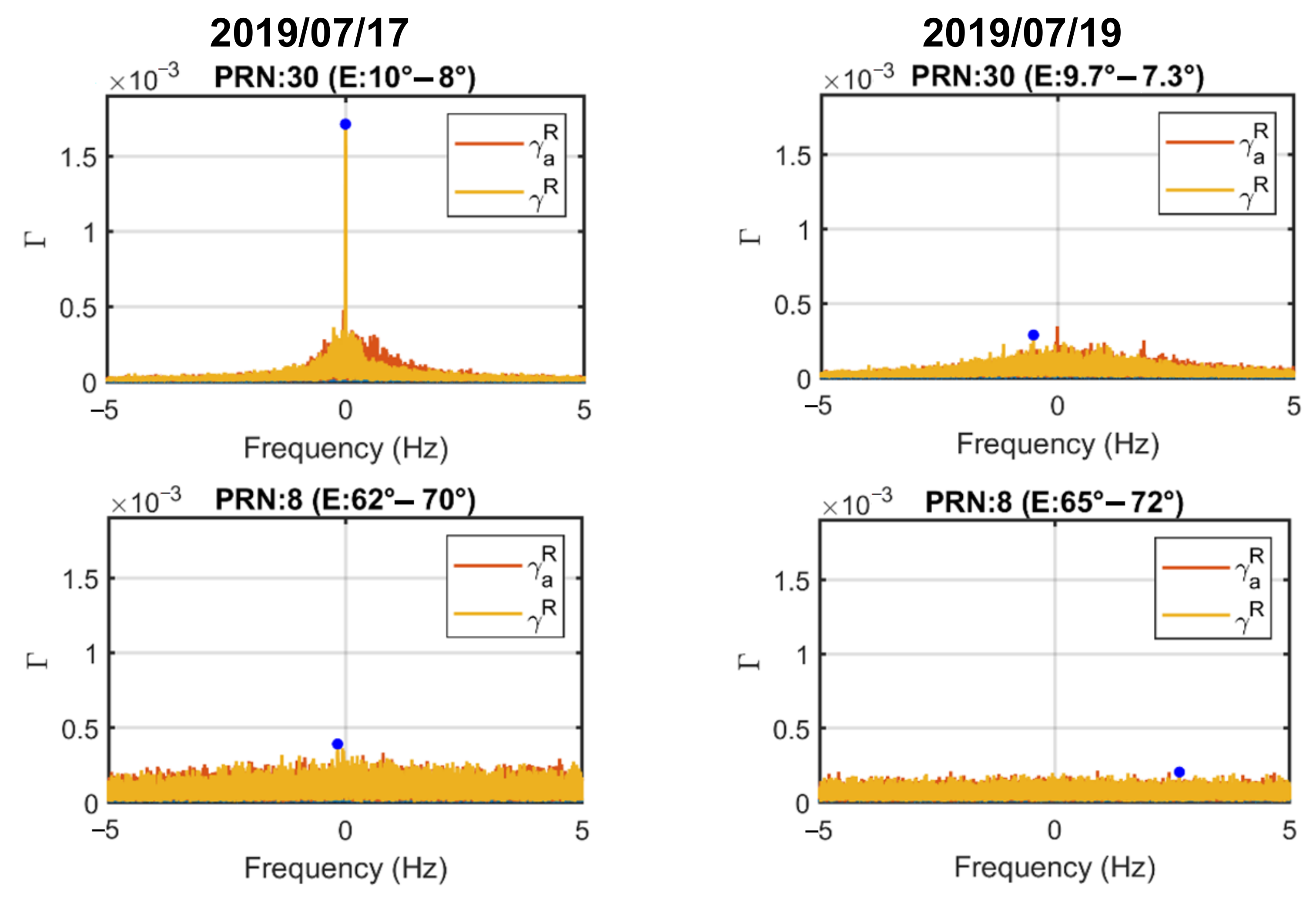
3.1.3. Spectral Retrievals
3.1.4. Residual Phase Retrieval and Tropospheric Residual Model
3.1.5. Zenith Total Delay Inversion
4. Results
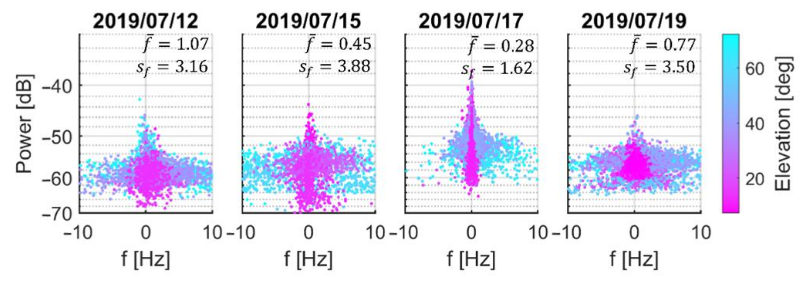
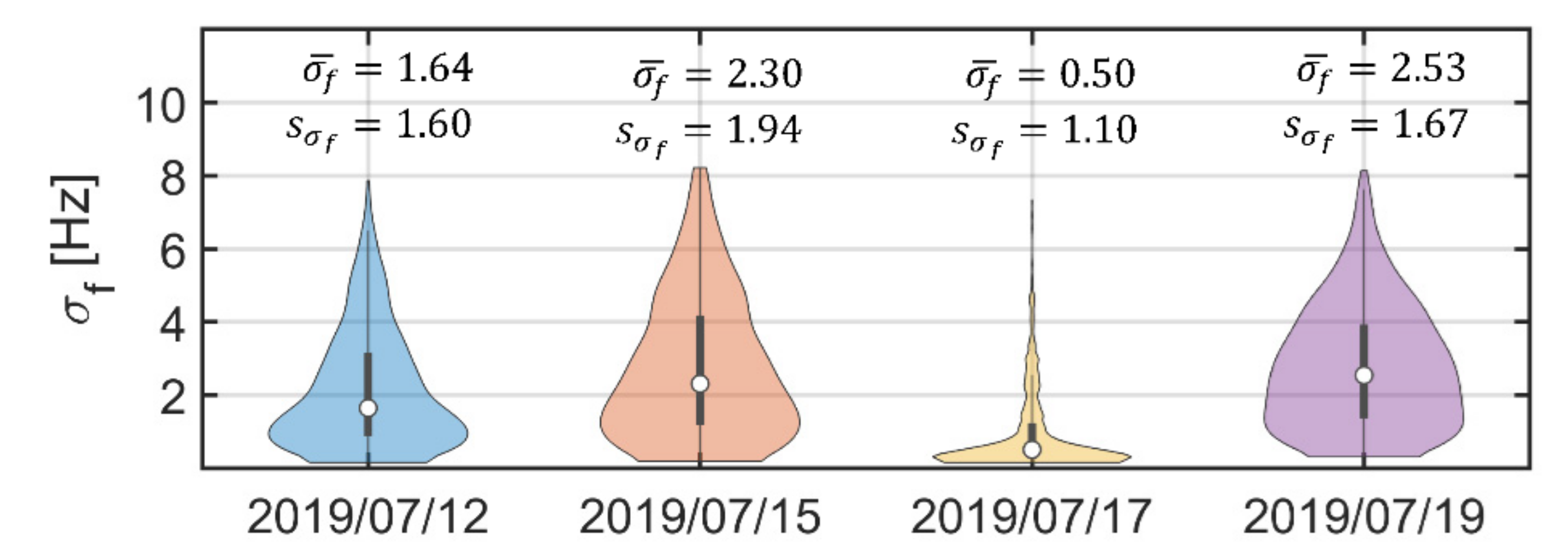
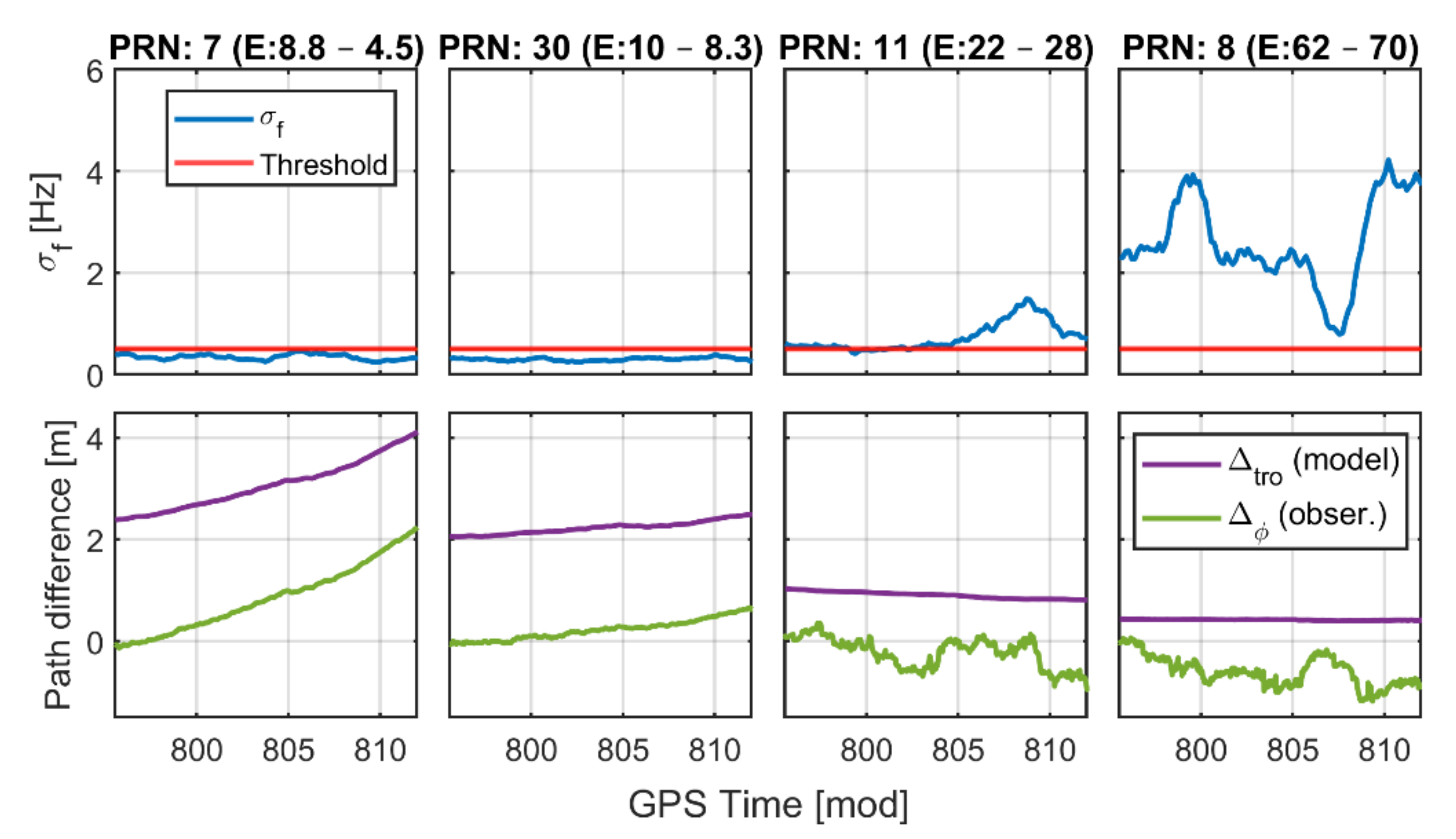
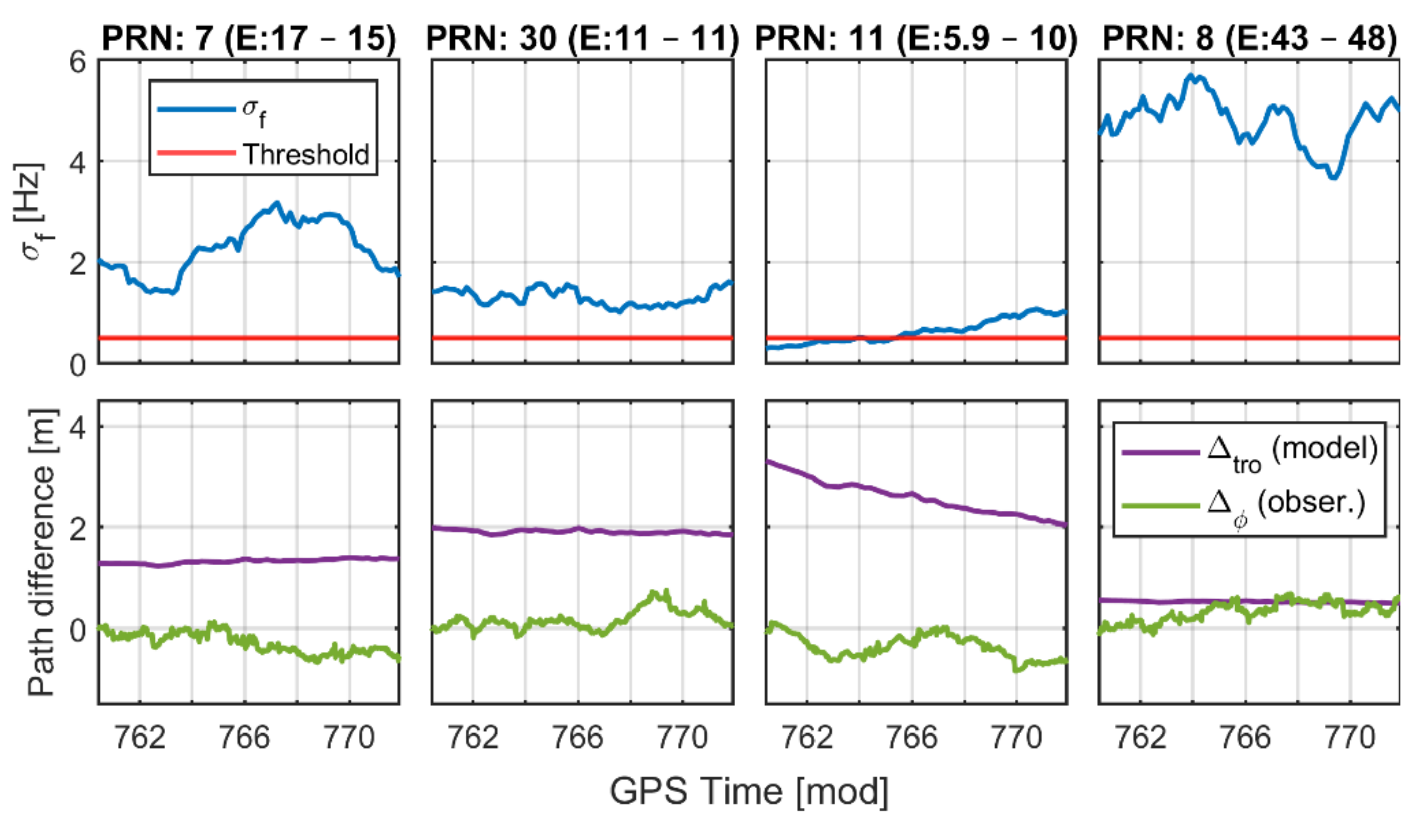
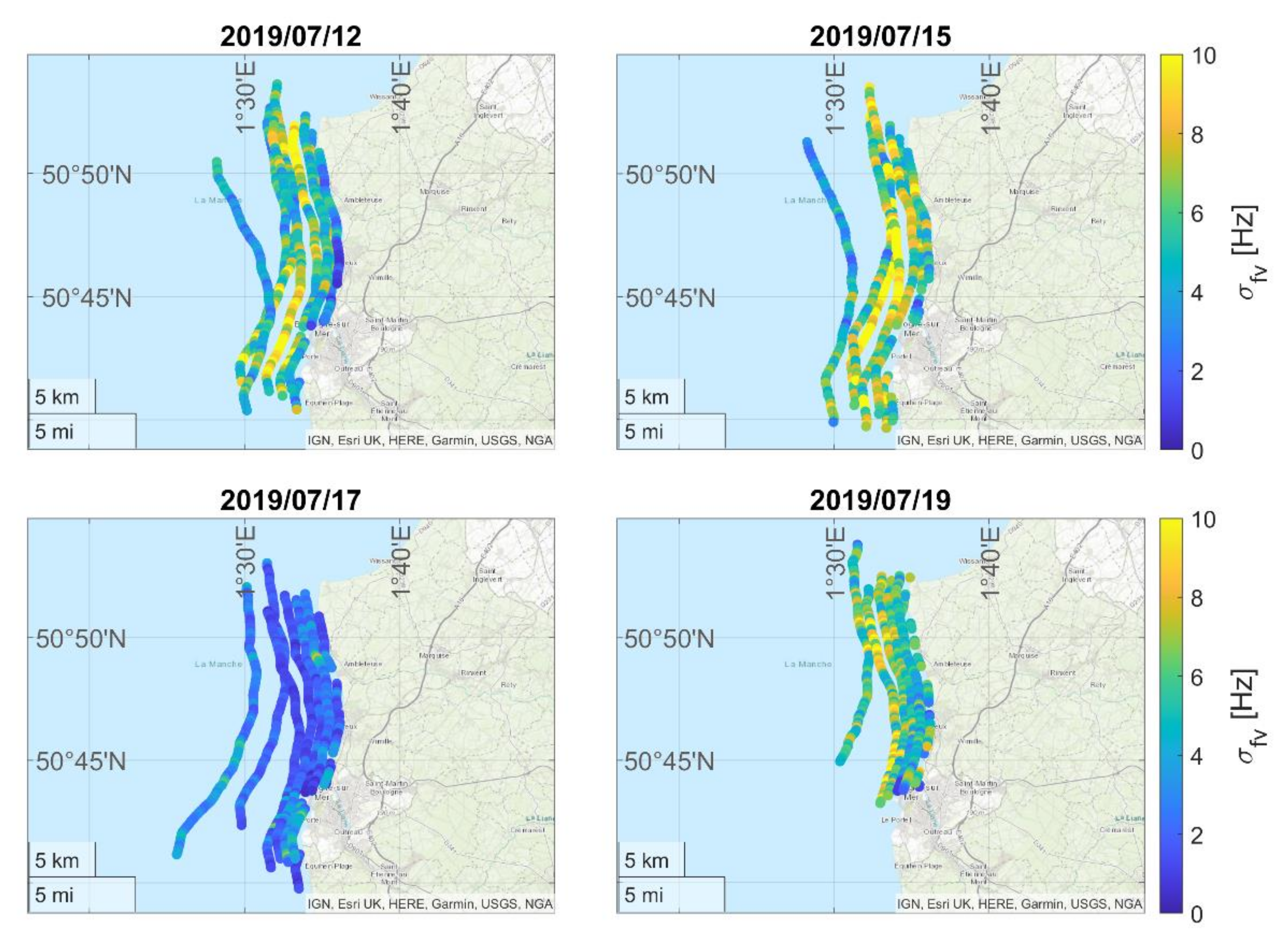
4.1. Results on Residual Doppler Spread
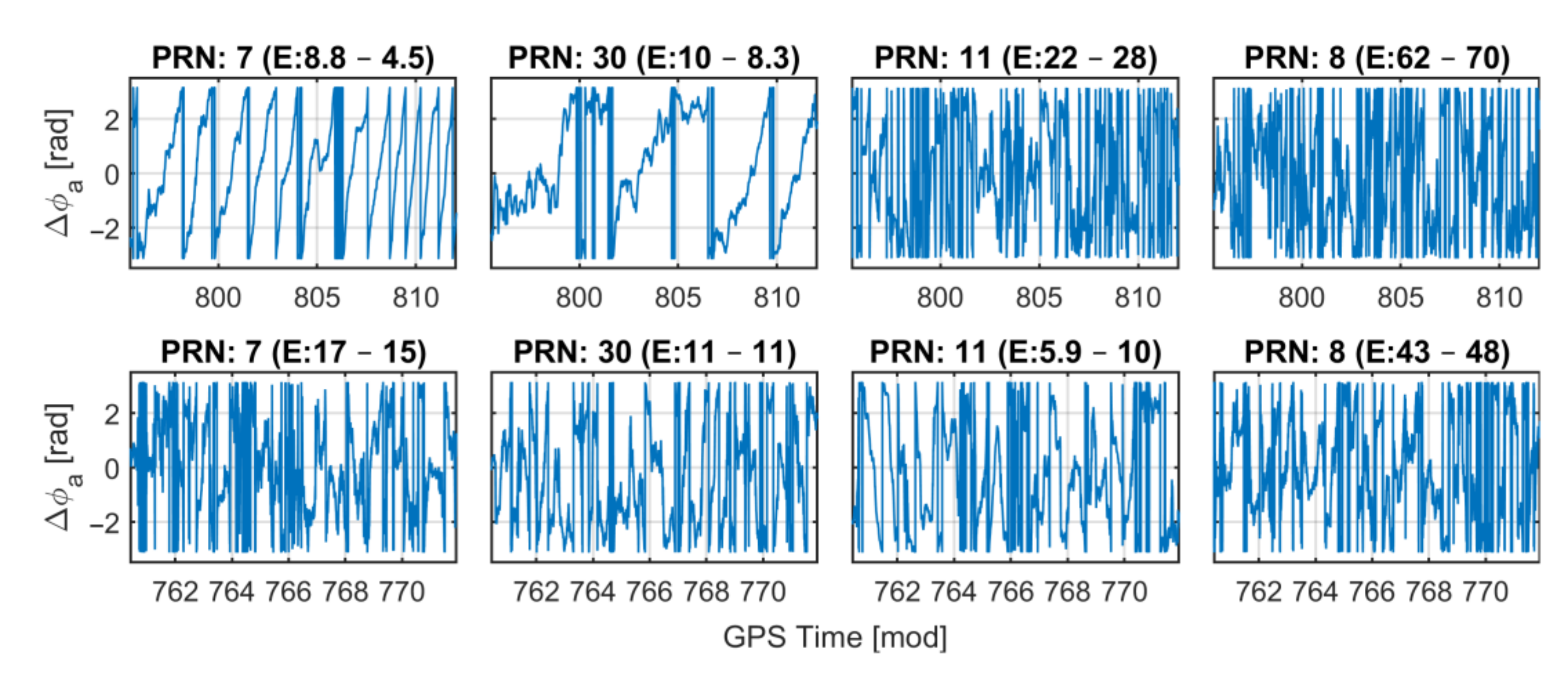
4.2. Results on Carrier Phase Retrieval
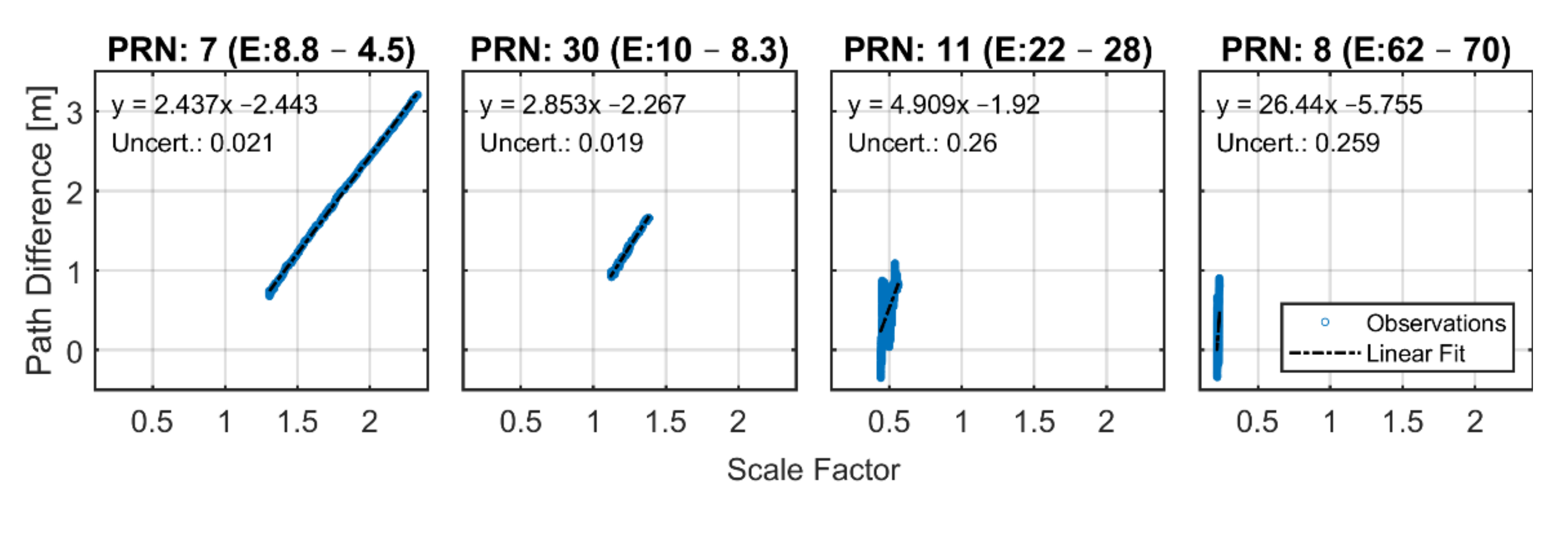
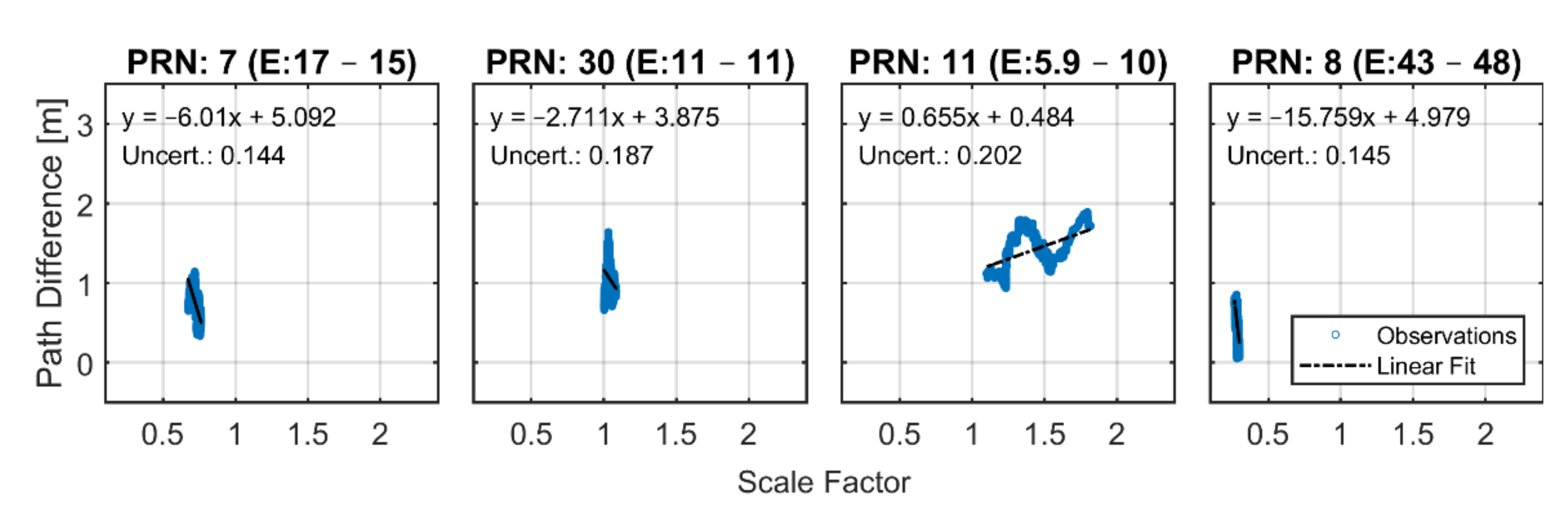
4.3. Results on Zenith Total Delay Inversion
5. Conclusions
Author Contributions
Funding
Data Availability Statement
Acknowledgments
Conflicts of Interest
References
- Cazenave, A.; Cozannet, G.L. Sea Level Rise and Its Coastal Impacts. Earth’s Future 2014, 2, 15–34. [Google Scholar] [CrossRef]
- ESA Climate Office. Sea State. Available online: https://climate.esa.int/en/projects/sea-state/ (accessed on 24 November 2021).
- Bengtsson, L.; Hodges, K.I.; Roeckner, E. Storm Tracks and Climate Change. J. Clim. 2006, 19, 3518–3543. [Google Scholar] [CrossRef]
- Melet, A.; Teatini, P.; Le Cozannet, G.; Jamet, C.; Conversi, A.; Benveniste, J.; Almar, R. Earth Observations for Monitoring Marine Coastal Hazards and Their Drivers. Surv. Geophys. 2020, 41, 1489–1534. [Google Scholar] [CrossRef]
- Benveniste, J.; Cazenave, A.; Vignudelli, S.; Fenoglio-Marc, L.; Shah, R.; Almar, R.; Andersen, O.; Birol, F.; Bonnefond, P.; Bouffard, J.; et al. Requirements for a Coastal Hazards Observing System. Front. Mar. Sci. 2019, 6, 348. [Google Scholar] [CrossRef]
- Martín-Neira, M. A Passive Reflectometry and Interferometry System (PARIS): Application to Ocean Altimetry. ESA J. 1993, 17, 331–355. [Google Scholar]
- Semmling, M.; Beyerle, G.; Beckheinrich, J.; Ge, M.; Wickert, J. Airborne GNSS Reflectometry Using Crossover Reference Points for Carrier Phase Altimetry. In Proceedings of the 2014 IEEE Geoscience and Remote Sensing Symposium, Quebec City, QC, Canada, 13–18 July 2014; pp. 3786–3789. [Google Scholar]
- Clarizia, M.P.; Ruf, C.; Cipollini, P.; Zuffada, C. First Spaceborne Observation of Sea Surface Height Using GPS-Reflectometry. Geophys. Res. Lett. 2016, 43, 767–774. [Google Scholar] [CrossRef]
- Cardellach, E.; Li, W.; Rius, A.; Semmling, M.; Wickert, J.; Zus, F.; Ruf, C.S.; Buontempo, C. First Precise Spaceborne Sea Surface Altimetry with GNSS Reflected Signals. IEEE J. Sel. Top. Appl. Earth Obs. Remote Sens. 2020, 13, 102–112. [Google Scholar] [CrossRef]
- Yan, Q.; Huang, W. Sea Ice Remote Sensing Using GNSS-R: A Review. Remote Sens. 2019, 11, 2565. [Google Scholar] [CrossRef]
- Munoz-Martin, J.F.; Perez, A.; Camps, A.; Ribó, S.; Cardellach, E.; Stroeve, J.; Nandan, V.; Itkin, P.; Tonboe, R.; Hendricks, S.; et al. Snow and Ice Thickness Retrievals Using GNSS-R: Preliminary Results of the MOSAiC Experiment. Remote Sens. 2020, 12, 4038. [Google Scholar] [CrossRef]
- Rodriguez-Alvarez, N.; Holt, B.; Jaruwatanadilok, S.; Podest, E.; Cavanaugh, K.C. An Arctic Sea Ice Multi-Step Classification Based on GNSS-R Data from the TDS-1 Mission. Remote Sens. Environ. 2019, 230, 111202. [Google Scholar] [CrossRef]
- Larson, K.M.; Small, E.E.; Gutmann, E.; Bilich, A.; Axelrad, P.; Braun, J. Using GPS Multipath to Measure Soil Moisture Fluctuations: Initial Results. GPS Solut. 2008, 12, 173–177. [Google Scholar] [CrossRef]
- Jia, Y.; Savi, P.; Pei, Y.; Notarpietro, R. GNSS Reflectometry for Remote Sensing of Soil Moisture. In Proceedings of the 2015 IEEE 1st International Forum on Research and Technologies for Society and Industry Leveraging a better tomorrow (RTSI), Torino, Italy, 16–18 September 2015; pp. 498–501. [Google Scholar]
- Calabia, A.; Molina, I.; Jin, S. Soil Moisture Content from GNSS Reflectometry Using Dielectric Permittivity from Fresnel Reflection Coefficients. Remote Sens. 2020, 12, 122. [Google Scholar] [CrossRef]
- Zavorotny, V.U.; Voronovich, A.G. Scattering of GPS Signals from the Ocean with Wind Remote Sensing Application. IEEE Trans. Geosci. Remote Sens. 2000, 38, 951–964. [Google Scholar] [CrossRef]
- Marchan-Hernandez, J.F.; Valencia, E.; Rodriguez-Alvarez, N.; Ramos-Perez, I.; Bosch-Lluis, X.; Camps, A.; Eugenio, F.; Marcello, J. Sea-State Determination Using GNSS-R Data. IEEE Geosci. Remote Sens. Lett. 2010, 7, 621–625. [Google Scholar] [CrossRef]
- Alonso-Arroyo, A.; Camps, A.; Park, H.; Pascual, D.; Onrubia, R.; Martin, F. Retrieval of Significant Wave Height and Mean Sea Surface Level Using the GNSS-R Interference Pattern Technique: Results from a Three-Month Field Campaign. IEEE Trans. Geosci. Remote Sens. 2015, 53, 3198–3209. [Google Scholar] [CrossRef]
- Foti, G.; Gommenginger, C.; Jales, P.; Unwin, M.; Shaw, A.; Robertson, C.; Roselló, J. Spaceborne GNSS Reflectometry for Ocean Winds: First Results from the UK TechDemoSat-1 Mission. Geophys. Res. Lett. 2015, 42, 5435–5441. [Google Scholar] [CrossRef]
- Jing, C.; Niu, X.; Duan, C.; Lu, F.; Di, G.; Yang, X. Sea Surface Wind Speed Retrieval from the First Chinese GNSS-R Mission: Technique and Preliminary Results. Remote Sens. 2019, 11, 3013. [Google Scholar] [CrossRef]
- Williams, S.D.P.; Nievinski, F.G. Tropospheric Delays in Ground-Based GNSS Multipath Reflectometry—Experimental Evidence from Coastal Sites. J. Geophys. Res. Solid Earth 2017, 122, 2310–2327. [Google Scholar] [CrossRef]
- Anderson, K.D. Determination of Water Level and Tides Using Interferometric Observations of GPS Signals. J. Atmos. Ocean. Technol. 2000, 17, 1118–1127. [Google Scholar] [CrossRef]
- Semmling, A.M.; Schmidt, T.; Wickert, J.; Schön, S.; Fabra, F.; Cardellach, E.; Rius, A. On the Retrieval of the Specular Reflection in GNSS Carrier Observations for Ocean Altimetry. Radio Sci. 2012, 47, RS6007. [Google Scholar] [CrossRef]
- Fabra, F.; Cardellach, E.; Rius, A.; Ribo, S.; Oliveras, S.; Nogues-Correig, O.; Belmonte Rivas, M.; Semmling, M.; D’Addio, S. Phase Altimetry with Dual Polarization GNSS-R Over Sea Ice. IEEE Trans. Geosci. Remote Sens. 2012, 50, 2112–2121. [Google Scholar] [CrossRef]
- Yan, Z.; Zheng, W.; Wu, F.; Wang, C.; Zhu, H.; Xu, A. Correction of Atmospheric Delay Error of Airborne and Spaceborne GNSS-R Sea Surface Altimetry. Front. Earth Sci. 2022, 10, 730551. [Google Scholar] [CrossRef]
- Nikolaidou, T.; Santos, M.; Williams, S.; Geremia-Nievinski, F. Development and Validation of Comprehensive Closed Formulas for Atmospheric Delay and Altimetry Correction in Ground-Based GNSS-R. TechRxiv 2022, preprint. [Google Scholar]
- Kucwaj, J.-C.; Reboul, S.; Stienne, G.; Choquel, J.-B.; Benjelloun, M. Circular Regression Applied to GNSS-R Phase Altimetry. Remote Sens. 2017, 9, 651. [Google Scholar] [CrossRef]
- Semmling, M. Altimetric Monitoring of Disko Bay Using Interferometric GNSS Observations on L1 and L2. Ph.D. Thesis, Deutsches GeoForschungsZentrum GFZ, Potsdam, Germany, 2012; 136p. [Google Scholar]
- Elfouhaily, T.; Thompson, D.R.; Linstrom, L. Delay-Doppler Analysis of Bistatically Reflected Signals from the Ocean Surface: Theory and Application. IEEE Trans. Geosci. Remote Sens. 2002, 40, 560–573. [Google Scholar] [CrossRef]
- Semmling, A.M.; Beyerle, G.; Stosius, R.; Dick, G.; Wickert, J.; Fabra, F.; Cardellach, E.; Ribó, S.; Rius, A.; Helm, A.; et al. Detection of Arctic Ocean Tides Using Interferometric GNSS-R Signals. Geophys. Res. Lett. 2011, 38, L04103. [Google Scholar] [CrossRef]
- Foerste, C.; Bruinsma, S.; Flechtner, F.; Marty, J.-C.; Dahle, C.; Abrykosov, O.; Lemoine, J.-M.; Neumayer, H.; Barthelmes, F.; Biancale, R.; et al. EIGEN-6C2—A New Combined Global Gravity Field Model Including GOCE Data up to Degree and Order 1949 of GFZ Potsdam and GRGS Toulouse. Geophys. Res. Abstr. EGU Gen. Assem. 2013, 15, 4077. [Google Scholar]
- Issa, H.; Stienne, G.; Reboul, S.; Raad, M.; Faour, G. Airborne GNSS Reflectometry for Water Body Detection. Remote Sens. 2021, 14, 163. [Google Scholar] [CrossRef]
- Zimmermann, F.; Schmitz, B.; Klingbeil, L.; Kuhlmann, H. GPS Multipath Analysis Using Fresnel Zones. Sensors 2018, 19, 25. [Google Scholar] [CrossRef]
- Semmling, A.M.; Wickert, J.; Schön, S.; Stosius, R.; Markgraf, M.; Gerber, T.; Ge, M.; Beyerle, G. A Zeppelin Experiment to Study Airborne Altimetry Using Specular Global Navigation Satellite System Reflections. Radio Sci. 2013, 48, 427–440. [Google Scholar] [CrossRef]
- ISO 2533:1975; Standard Atmosphere. International Organization for Standardization: Geneva, Switzerland, 1975.
- Treuhaft, R.N.; Lowe, S.T.; Zuffada, C.; Chao, Y. 2-cm GPS Altimetry over Crater Lake. Geophys. Res. Lett. 2001, 28, 4343–4346. [Google Scholar] [CrossRef]
- Landskron, D.; Böhm, J. VMF3/GPT3: Refined Discrete and Empirical Troposphere Mapping Functions. J. Geod. 2018, 92, 349–360. [Google Scholar] [CrossRef]
- Böhm, J.; Boisits, J. re3data.org: VMF Data Server; Department of Geodesy and Geoinformation, TU Wien: Vienna, Austria, 2016. [Google Scholar] [CrossRef]
- Wang, Y.; Breitsch, B.; Morton, Y.T.J. A State-Based Method to Simultaneously Reduce Cycle Slips and Noise in Coherent GNSS-R Phase Measurements From Open-Loop Tracking. IEEE Trans. Geosci. Remote Sens. 2021, 59, 8873–8884. [Google Scholar] [CrossRef]
- Hersbach, H.; Bell, B.; Berrisford, P.; Biavati, G.; Horányi, A.; Muñoz Sabater, J.; Nicolas, J.; Peubey, C.; Radu, R.; Rozum, I.; et al. ERA5 Hourly Data on Single Levels from 1979 to Present. Available online: https://cds.climate.copernicus.eu/cdsapp#!/dataset/reanalysis-era5-single-levels?tab=overview (accessed on 11 December 2021).
- Wang, Y.; Liu, Y.; Roesler, C.; Morton, Y.J. Detection of Coherent GNSS-R Measurements Using a Support Vector Machine. In Proceedings of the IGARSS 2020–2020 IEEE International Geoscience and Remote Sensing Symposium, Waikoloa, HI, USA, 26 September–2 October 2020; pp. 6210–6213. [Google Scholar]
- Kačmařík, M. Retrieving of GNSS Tropospheric Delays from RTKLIB in Real-Time and Post-Processing Mode. In Dynamics in GIscience, Proceedings of the GIS Ostrava, Ostrava, Czech Republic, 22–24 March 2017; Ivan, I., Horák, J., Inspektor, T., Eds.; Springer International Publishing: Cham, Switzerland, 2018; pp. 181–194. [Google Scholar]
- Li, W.; Cardellach, E.; Fabra, F.; Ribó, S.; Rius, A. Lake Level and Surface Topography Measured with Spaceborne GNSS-Reflectometry from CYGNSS Mission: Example for the Lake Qinghai. Geophys. Res. Lett. 2018, 45, 13332–13341. [Google Scholar] [CrossRef]
- Semmling, A.M.; Beckheinrich, J.; Wickert, J.; Beyerle, G.; Schön, S.; Fabra, F.; Pflug, H.; He, K.; Schwabe, J.; Scheinert, M. Sea Surface Topography Retrieved from GNSS Reflectometry Phase Data of the GEOHALO Flight Mission. Geophys. Res. Lett. 2014, 41, 954–960. [Google Scholar] [CrossRef]
- Wang, Y.; Morton, Y.J. Ionospheric Total Electron Content and Disturbance Observations from Space-Borne Coherent GNSS-R Measurements. IEEE Trans. Geosci. Remote Sens. 2022, 60, 5801013. [Google Scholar] [CrossRef]


| Date | Wind Speed (m/s) | Wind Direction (deg) | SWH (m) |
|---|---|---|---|
| 12 July 2019 | 5.49 | 117 | 0.30 |
| 15 July 2019 | 4.29 | 67 | 0.58 |
| 17 July 2019 | 2.92 | 204 | 0.26 |
| 19 July 2019 | 6.50 | 240 | 0.55 |
| Parameter | Low | Mid | High |
|---|---|---|---|
| Wind Speed | 0.88 | 0.66 | 0.58 |
| SWH | 0.75 | 0.58 | 0.56 |
| Threshold | Low | Mid | High |
|---|---|---|---|
| 10% | 5% | 0% |
Publisher’s Note: MDPI stays neutral with regard to jurisdictional claims in published maps and institutional affiliations. |
© 2022 by the authors. Licensee MDPI, Basel, Switzerland. This article is an open access article distributed under the terms and conditions of the Creative Commons Attribution (CC BY) license (https://creativecommons.org/licenses/by/4.0/).
Share and Cite
Moreno, M.; Semmling, M.; Stienne, G.; Dalil, W.; Hoque, M.; Wickert, J.; Reboul, S. Airborne Coherent GNSS Reflectometry and Zenith Total Delay Estimation over Coastal Waters. Remote Sens. 2022, 14, 4628. https://doi.org/10.3390/rs14184628
Moreno M, Semmling M, Stienne G, Dalil W, Hoque M, Wickert J, Reboul S. Airborne Coherent GNSS Reflectometry and Zenith Total Delay Estimation over Coastal Waters. Remote Sensing. 2022; 14(18):4628. https://doi.org/10.3390/rs14184628
Chicago/Turabian StyleMoreno, Mario, Maximilian Semmling, Georges Stienne, Wafa Dalil, Mainul Hoque, Jens Wickert, and Serge Reboul. 2022. "Airborne Coherent GNSS Reflectometry and Zenith Total Delay Estimation over Coastal Waters" Remote Sensing 14, no. 18: 4628. https://doi.org/10.3390/rs14184628
APA StyleMoreno, M., Semmling, M., Stienne, G., Dalil, W., Hoque, M., Wickert, J., & Reboul, S. (2022). Airborne Coherent GNSS Reflectometry and Zenith Total Delay Estimation over Coastal Waters. Remote Sensing, 14(18), 4628. https://doi.org/10.3390/rs14184628