Abstract
Data assimilation (DA) is often used for merging observations to improve the predictions of the current and future states of characteristics of interest. In forest inventory, DA has so far found limited use, although dense time series of remotely sensed (RS) data have become available for estimating forest characteristics. A problem in forest inventory applications based on RS data is that errors from subsequent predictions tend to be strongly correlated, which limits the efficiency of DA. One reason for such a correlation is that model-based predictions, using techniques such as parametric or non-parametric regression, are normally biased conditional on the actual ground conditions, although they are unbiased conditional on the RS predictor variables. A typical case is that predictions are shifted towards the mean, i.e., small true values are overestimated, and large true values are underestimated. In this study, we evaluated if the classical calibration of RS-based predictions could remove this type of bias and improve DA results. Through a simulation study, we mimicked growing stock volume predictions from two different sensors: one from a metric strongly correlated with growing stock volume, mimicking airborne laser scanning, and one from a metric slightly less correlated with growing stock volume, mimicking data obtained from 3D digital photogrammetry. Consistent with previous findings, in areas such as chemistry, we found that classical calibration made the predictions approximately unbiased. Further, in most cases, calibration improved the DA results, evaluated in terms of the root mean square error of predicted volumes, evaluated at the end of a series of ten RS-based predictions.
1. Introduction
Data assimilation (DA) has been used for a long time in areas such as meteorology and robotics for merging new observations with existing information [1,2,3]. The typical objectives are to estimate the current state of a system as precisely as possible and to make forecasts about future states. In forest inventory, DA has found limited use, although, e.g., [4,5,6] proposed its use several decades ago. The Kalman filter [7] is a standard method to implement DA; it combines the model predictions of a state variable with repeated measurements across a period of interest. Czaplewski et al. [5] suggested that the Kalman filter could be suitable for monitoring forest cover. Dixon and Howitt [4] proposed that it could be applied in stand-level forest inventories by forecasting old inventory estimates and combining them with new estimates. Kangas [6] used the Kalman filter in connection with estimating the growing stock volume in the Finnish national forest inventory.
It has been argued that DA could be a straightforward approach for making appropriate use of dense time series of remotely sensed (RS) data, for acquiring precise and up-to-date information for forest planning [8,9]. However, initial empirical studies have identified several obstacles that need to be solved before the technique can be efficiently adopted into practice [10,11]. This involves, e.g., the need for calibrating predictions to remove bias and handling correlated prediction errors [12]. By developing a modified DA filter, [13] demonstrated substantial improvements compared to previous empirical studies.
When DA is based on a sequence of RS data, the typical procedure applied in empirical studies (e.g., [10,11]) involves the following steps:
- (1)
- An initial prediction of the variable of interest is made using a model obtained through regressing field reference data on RS metrics with the same spatial resolution.
- (2)
- A growth model is applied to predict the development of the state until the next RS data acquisition time point.
- (3)
- A new RS-based prediction is obtained, as described in step (1). This prediction is merged with the forecast from step (2) based on the uncertainty of the two predictions. With the standard Kalman filter, the two predictions are merged through a weighting procedure, which assigns weights inversely proportional to their variances.
- (4)
- Following the merger of the two predictions in step (3), the DA procedure continues by applying a growth model to the merged prediction to forecast the state to the next RS data acquisition time point.
- (5)
- A new RS-based prediction is merged with the forecasted prediction from step (4) through the procedure described in step (3). Steps (4) and (5) are repeated as many times as there are new predictions to assimilate.
Other approaches to DA in forest inventories exist as well, e.g., [14].
RS data from a variety of sensors can be applied (e.g., [13]), such as airborne laser scanning (ALS) and 3D digital aerial photogrammetry (DP). Different sensors acquire data from the forest in different ways, and some, such as ALS, have been shown to be more suitable than others for predicting common forest variables, such as growing stock volume (GSV) and biomass. Due to the different properties of RS data, the accuracy of RS-based predictions varies; this is due both to sensor properties and to specific atmospheric and other conditions prevailing during the acquisition. The reported relative root mean square errors (%RMSEs) for GSV predictions at sample plot level (order of size 300 m2) under Nordic conditions typically range between 20 and 30% for predictions based on DP data and between 15 and 20% for predictions based on ALS data (e.g., [15,16,17]).
DA routines in different fields of application require issues pertinent to the particular field to be handled properly. As identified by [12], one such issue, when DA is based on predictions of forest characteristics from RS data, is that the prediction errors from models applied at different time points tend to be strongly positively correlated. Consequently, a new prediction adds only a limited amount of new information, and the standard Kalman filter performs poorly since it assumes new predictions are uncorrelated with previous predictions.
The reasons for correlated errors are several. One reason is that a specific sensor type is likely to respond in a similar way at different time points to some specific forest conditions, such as dense or sparse tree foliage, dense or sparse non-tree vegetation, or specific topographical or hydrological conditions. Therefore, predictions for a given plot at different time points will tend to have prediction errors with the same sign and magnitude, i.e., they will be positively correlated. Another important reason for positively correlated errors is that the predictions are based on models. Although predictions from parametric and non-parametric regression models are normally approximately unbiased, conditional on the RS explanatory variables, they are normally biased, conditional on the true state of the characteristic of interest (e.g., [18]). In areas such as chemistry, compensating for such bias is a standard procedure while performing instrument calibration (ibid.). However, the use of a similar calibration to make predictions unbiased conditional on the true ground conditions is seldom applied in forest remote sensing studies (cf., [13,19]), and as a result, small true values tend to be overestimated, and large true values underestimated. In a model-based setting, this implies correlated prediction errors.
The latter cause of correlation is prominent, especially if the underlying RS data correlate only weakly with the dependent variable, e.g., when GSV is predicted from optical satellite data [20,21]. With RS data that correlate strongly with the dependent variable, the problem is less pronounced, e.g., when GSV is predicted from airborne laser scanning data [22,23,24]. Note that this does not imply that the models have been incorrectly specified or estimated. Instead, this effect is an inherent feature of regression analysis and similar machine learning techniques since they are designed to predict the correct value on average, conditional on the input variables [25], i.e., the RS data in our case. They are not designed to provide unbiased predictions conditional on the true value, although this would be desirable for DA applications. As a result, when non-calibrated predictions based on different types of RS data have been merged, the improvements obtained by applying DA have been smaller than expected, and in some extreme cases, had a negative impact [11].
In this study, we propose and evaluate a standard calibration approach for mitigating the negative effects in DA applications of RS-based predictions exhibiting shifts towards the mean. The method applied is based on classical calibration methods [18,26,27] to make RS-based predictions approximately unbiased conditional on the true value of the variable of interest. The method has previously been used as part of a DA routine applied to empirical data by [13]. In this study, we provide the background for its application and results from different sequences of simulated RS data. We assume two different, fictitious RS sensors, one mimicking ALS and the other mimicking DP, which allows us to explore the effects on the DA of different sensor properties with regard to prediction accuracy and error correlation. To single out the effects of calibration, the time between successive data acquisitions was specified to be short, and thus growth updates were not required as part of the DA routine.
2. Materials and Methods
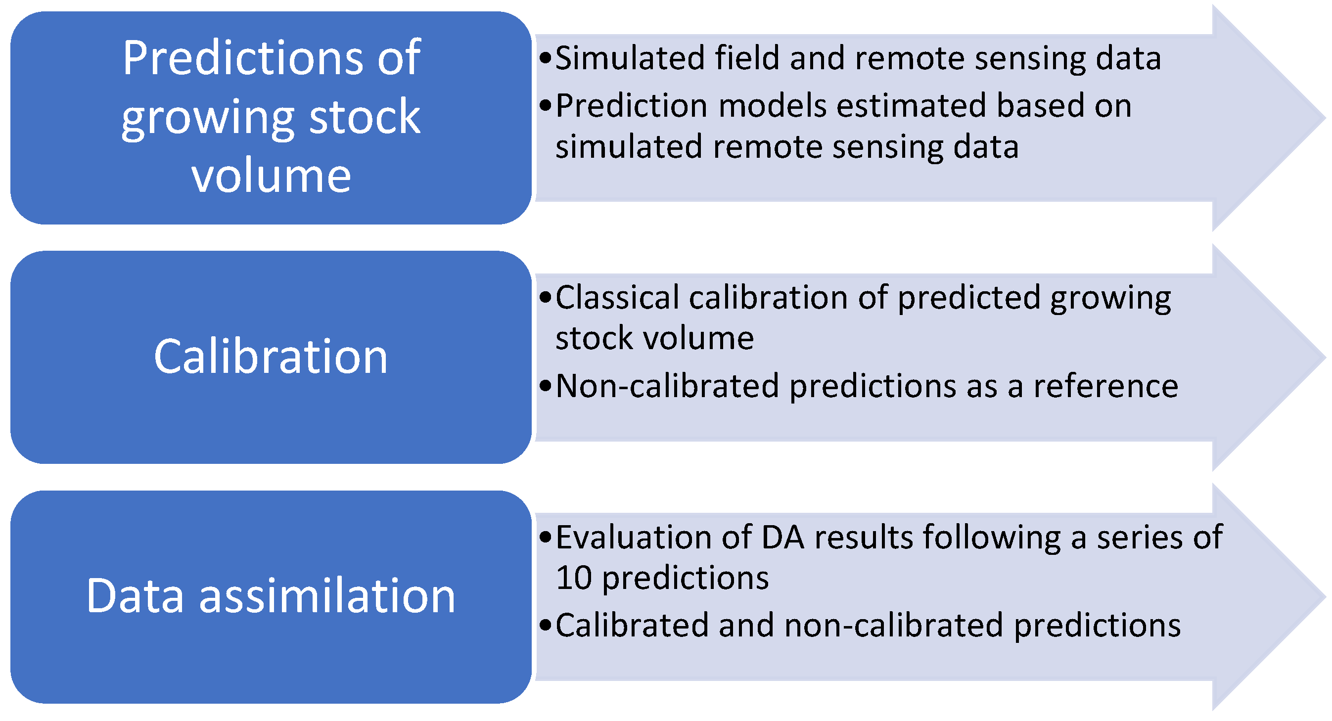
The study was conducted as a simulation study at the level of plots, assumed to be about 300 m2 large. The plots were assumed to be inventoried in the field with regard to GSV and georeferenced so that remote sensing metrics could be matched with field reference data. Based on the field data, we simulated RS metrics mimicking ALS and DP, founded on empirical evidence from previous studies. Models predicting GSV from RS data were developed and subsequently calibrated before being applied in DA, using a DA filter that accounted for correlation between predictions, e.g., [13]. Figure 1 provides an overview of the study.
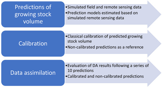
Figure 1.
An overview of the different parts of the study.
2.1. Simulating the Population
The simulations were set up to mimic GSV values from forest plots and the corresponding RS metrics from ALS and DP from such plots. The empirical basis for the simulation study was taken from the Swedish National Forest Inventory (e.g., [28]) with regard to the approximate range of GSV values at the plot level. However, we deliberately left out low GSV values to avoid young forests and clear-cut areas, in which non-standard calibration procedures would be required to avoid negative values after calibration. The GSV values, T (m3ha−1), at the level of the sample plots were simulated independently from a gamma distribution, with a mean value of 150 and a standard deviation of 60, as a flexible means of forming a population of 5000 units. Several datasets of a similar kind were simulated, for DA applications using ALS and DP data in a series of 10 acquisitions. Further, for each sensor and time point, two different datasets were simulated, one for estimation and one for independent validation of the estimated models and results of DA procedures.
The next step involved simulating RS data linked to the GSV values (in all the datasets), mimicking ALS and DP. The generic model used for this purpose was similar to the one used by [29] for predicting biomass from 3D data. The model applied was:
In this model, is the ALS or DP metric intended to mimic a metric related to the product of tree height and vegetation cover, and i is the true GSV value. The -parameters were assigned separately for ALS and DP (see Table 1). The error terms were specified to be normally distributed and expressed in vector format as , with being a diagonal matrix containing weights to allow heteroscedasticity. To simulate mild heteroscedasticity, we assigned the weights in as . The parameters for the generation of ALS and DP metrics according to Equation (1) are given in Table 1.

Table 1.
Input parameters for simulating the relationship between GSV and RS metrics according to Equation (1).
From previous studies, we know that plot level RS metrics obtained in a time sequence tend to have serially correlated error terms [12]. To simulate such error terms based on Equation (1), we used the Cholesky decomposition method [30]. Thus, the RS metrics from all ten acquisitions in a specific series for both sensors were generated simultaneously. The specified correlations are given in Table 2.

Table 2.
Specified plot level correlations between the error terms according to Equation (1) for a given sensor and the corresponding cross-correlation between sensors.
As shown in Table 2, the two different cases regarding the correlations of the error terms in Equation (1) were investigated. In the first case, the error terms were specified as fully uncorrelated. In the second case, we specified a certain plot level serial correlation between the error terms for a given sensor, as well as across sensors. All pairs of error terms in a time series were specified to obtain the same correlation; for a given plot, the correlation was the same between the first and the second acquisition as between the first and the last acquisition. This was motivated by the short time period during which the RS data were assumed to be acquired.
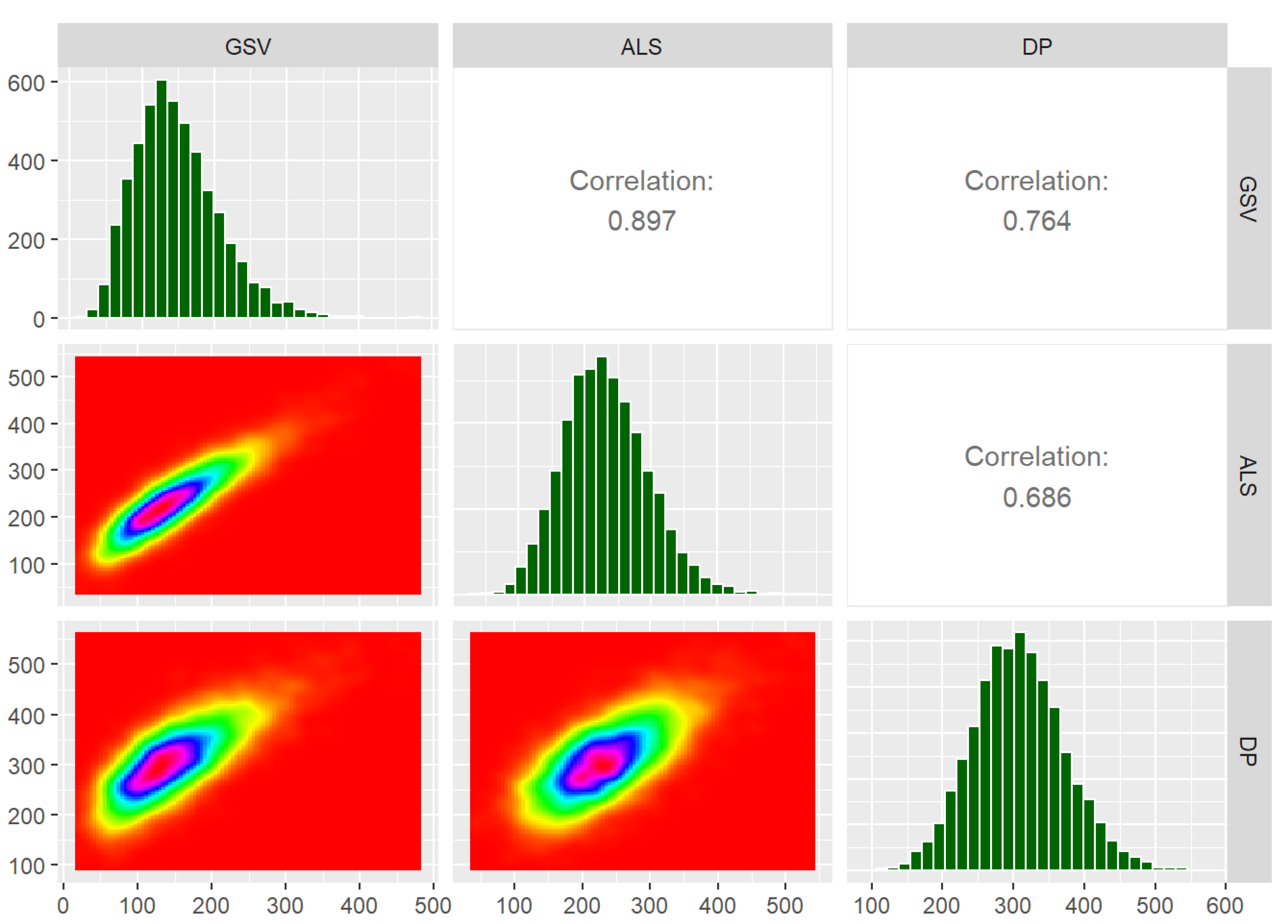
Following the steps described above, simulated field and RS metrics mimicking real conditions were available. In Figure 2, these metrics and the dependencies between them are summarised in terms of scatterplots, histograms, and correlations, based on the first validation dataset from each group of ten ALS and DP datasets. Note that the correlations reported in Figure 2 are the empirical correlations between the variables, i.e., not the correlations between the error terms (which are reported in Table 2).
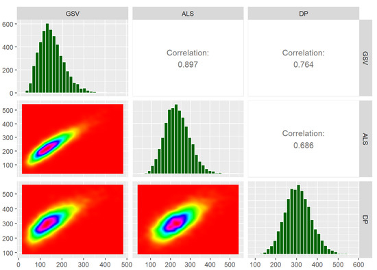
Figure 2.
Summary of simulated data. GSV is the plot level growing stock volume (m3ha−1), ALS is the metric from airborne laser scanning, and DP is the metric from digital aerial photogrammetry.
2.2. GSV Prediction Models
Based on the simulated data, models predicting GSV from RS metrics were specified and estimated. The following non-linear model form was specified for both ALS and DP metrics:
Here, the terms are parameters and the term is the residual error term with zero expectation and potentially heterogeneous variance. Since the RS metric () reflects a (transformed) product of vegetation height and cover, this model form has previously been used in modelling GSV and biomass from ALS and DP metrics (e.g., [29]). For computational reasons and simpler interpretation, since a separate model was estimated for a large number of datasets in repeated simulations, we avoided a non-linear model and performed model fitting through a non-linear least squares iterative estimation by first investigating what would be a good choice of for a transformation . For ALS and DP data generated according to the description in the previous section, initial studies indicated that was suitable and thus was applied in the simple linear model:
The model parameters of Equation (3) were estimated using ordinary least-squares regression in R [31] separately for each dataset designated for model estimation. In Table 3, the summary statistics of the estimated models are presented (for the models estimated based on the first of the ten datasets designated for estimation, based on data with non-correlated residual errors).

Table 3.
Estimated model parameters according to Equation (3) based on ALS and DP data.
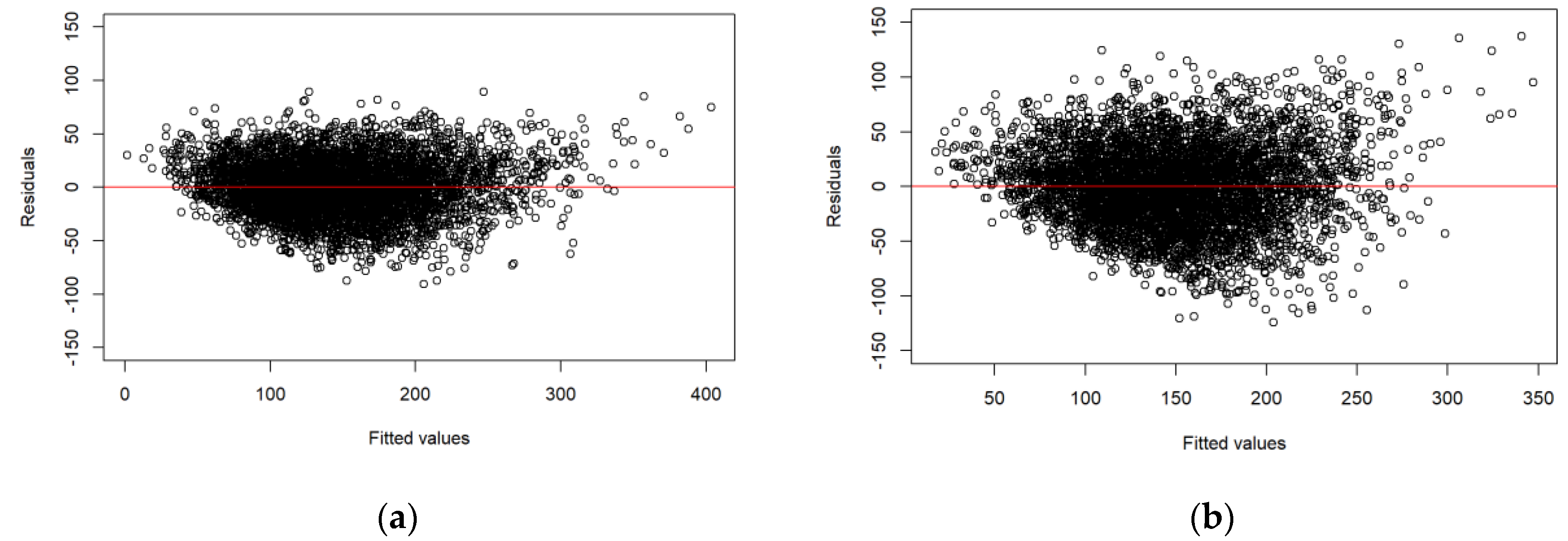
Figure 3 shows the residual plots for the models displayed in Table 3. No trend of residuals over fitted values could be observed, except for slightly heteroscedastic residual variance.
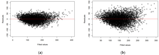
Figure 3.
Residual plots: (a) the model based on ALS data; (b) the model based on DP data.
The estimated models were applied to each of the datasets designated for validation to predict GSV values from the RS metrics. Residual terms were extracted to compute the average RMSE for the ALS and DP datasets and to compute the average plot level residual error correlation across different datasets. These statistics are given in Table 4.

Table 4.
Relative root mean square errors (%RMSEs) and plot level residual correlations between predictions using the same sensor and across sensors.
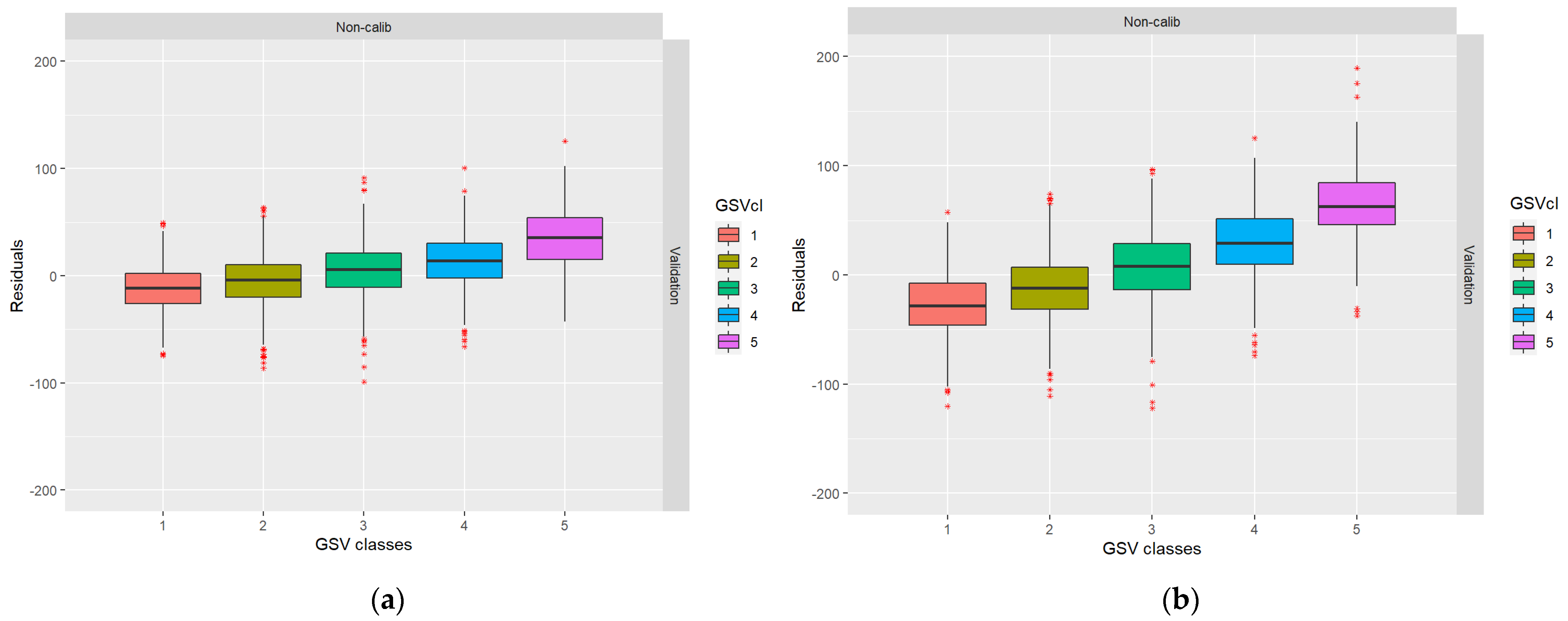
From Table 4, it can be noted that even in case I, when the residuals of the RS metrics were simulated as independent between datasets, residual error correlations exist after the GSV predictions. This is due to the shift towards the mean described in the introduction (cf., [12]). In Figure 4, the boxplots show that low GSV values were overestimated and high GSV values were underestimated, as is ordinarily the case in regression analysis. The data for Table 3 and Figure 3 were taken from the first ALS and DP validation datasets for case I.

Figure 4.
Boxplots showing the distribution of residuals across the range of true values: (a) ALS-based residuals; (b) DP-based residuals.
2.3. Calibration
As an initial step for the calibration, we specified a linear error characterisation model (ECM, e.g., [18,19,32]) and estimated its parameters. This model is sometimes called the calibration model [18]. The ECM links RS-based predictions as the dependent variable with true GSV values as the explanatory variable. It displays the logical relationship between RS-based predictions and true GSV values when a certain sensor is applied at a given time point. The ECM is given as:
where is a predicted GSV value based on a fitted version of Equation (3), and are model coefficients, and is a random error term with zero expectation. Persson and Ståhl [19] showed how the estimated ECM can be used for a detailed description of the error properties of RS-based predictions, e.g., how their bias (conditional on the true GSV) vary across the range of true values. The model also forms the basis for classical calibration (e.g., [18,27,33]). The estimated ECM is:
which suggests that RS-based predictions can be calibrated by rearranging Equation (5) as:
where is a calibrated prediction. The properties of classical calibration have been assessed in several studies (e.g., [18,27]). In the following, we present approximate results for the expected value and variance of the calibration predictor. Since it is a ratio predictor, exact results cannot be obtained and the results we provide require that is strictly non-zero. Tellinghuisen [18] showed how detailed results can be obtained following a conditioning approach. The approximate expected value of the calibration predictor, assuming Equation (4) is a correctly specified model, is:
That is, the expected value of the calibrated GSV is approximately equal to the true GSV, which is an attractive property for DA applications. The approximate variance, assuming Equation (4) is a correctly specified model with homogeneous error variance, is:
More exact approximations can be obtained through Taylor series expansion, as shown by [18,33] for applications in chemometrics, but for the purpose of our study, the simple approximation provided above is sufficient since variances for determining weights in DA applications (shown later in this paper) were assessed empirically from the data rather than through Equation (8). Note that according to Equation (8), the variance increases following calibration if and decreases if . Typically, , and thus the variance of the predictions increases following calibration. In our study, all predictions in both of the datasets (estimation and validation) were calibrated, following the estimation of the coefficients of the ECM based on the datasets designated for estimation.
In Table 5, the relative RMSEs and correlations are given for the predicted values that have been calibrated. In Figure 5, the corresponding boxplots are given based on the first ALS and DP datasets designated for validation.

Table 5.
Post-calibration relative root mean square errors (%RMSEs) and plot level residual correlations between predictions using the same sensor and across sensors.
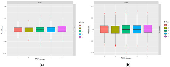
Figure 5.
Post-calibration boxplots showing the distribution of residuals across the range of true values: (a) ALS-based residuals; (b) DP-based residuals.
It can be observed in Figure 5 that the calibration makes the predictions approximately unbiased at the expense of larger residual variance. Further, from Table 5, it can be observed that the correlations between model residual errors in subsequent predictions are back to the levels initially assigned. However, the RMSEs of the calibrated predictions are larger than the non-calibrated predictions.
2.4. Data Assimilation
Using both calibrated and non-calibrated predictions for each of the sensors, we evaluated three different DA schemes, each involving ten assimilation steps. The three schemes were:
- (i)
- DA based on a series of 10 ALS-based predictions, using data with and without correlation between model residual errors in Equation (1).
- (ii)
- DA based on a series of 10 DP-based predictions, using data with and without correlation between model residual errors in Equation (1).
- (iii)
- DA based on a first ALS-based prediction, followed by a series of eight DP-based predictions, and ending with an ALS-based prediction, using data with and without model residual errors in Equation (1).
The third scheme was included since previous experience from [11] has shown that adding imprecise predictions after a first precise prediction may lead to worse assimilated predictions compared to using only the first prediction and a growth model. Thus, it is of interest to study if small amounts of less frequent (and typically expensive) data (ALS in our study) could be successfully assimilated with larger amounts of more frequent (and typically less expensive) data (DP in our study), when calibration is applied. To single out the effect of calibration, no growth updates were included in this study, i.e., it was assumed that all data were acquired within the same season.
The data assimilation principle applied was a modified Kalman filter, accounting for correlations between subsequent predictions [13]. Two predictions, either calibrated or non-calibrated, denoted and , where is either the first prediction in a series or a prediction obtained through DA at the previous stage, were linearly combined as:
where is the assimilated prediction and is a weight between 0 and 1. Equation (9) was applied until all the 10 predictions in a series were assimilated. The weight, , at each stage was determined as:
which minimizes the variance of the DA prediction (e.g., [13]). The variances and covariances involved were determined empirically by comparing predicted values with true values in the datasets designated for model estimation. With small datasets, the use of this type of empirically determined variance may sometimes be inappropriate (e.g., [34]), but in our case, the datasets were large enough for estimating the variances and covariances with high precision. For the computations, we used the R package ‘DatAssim’ [35].
3. Results
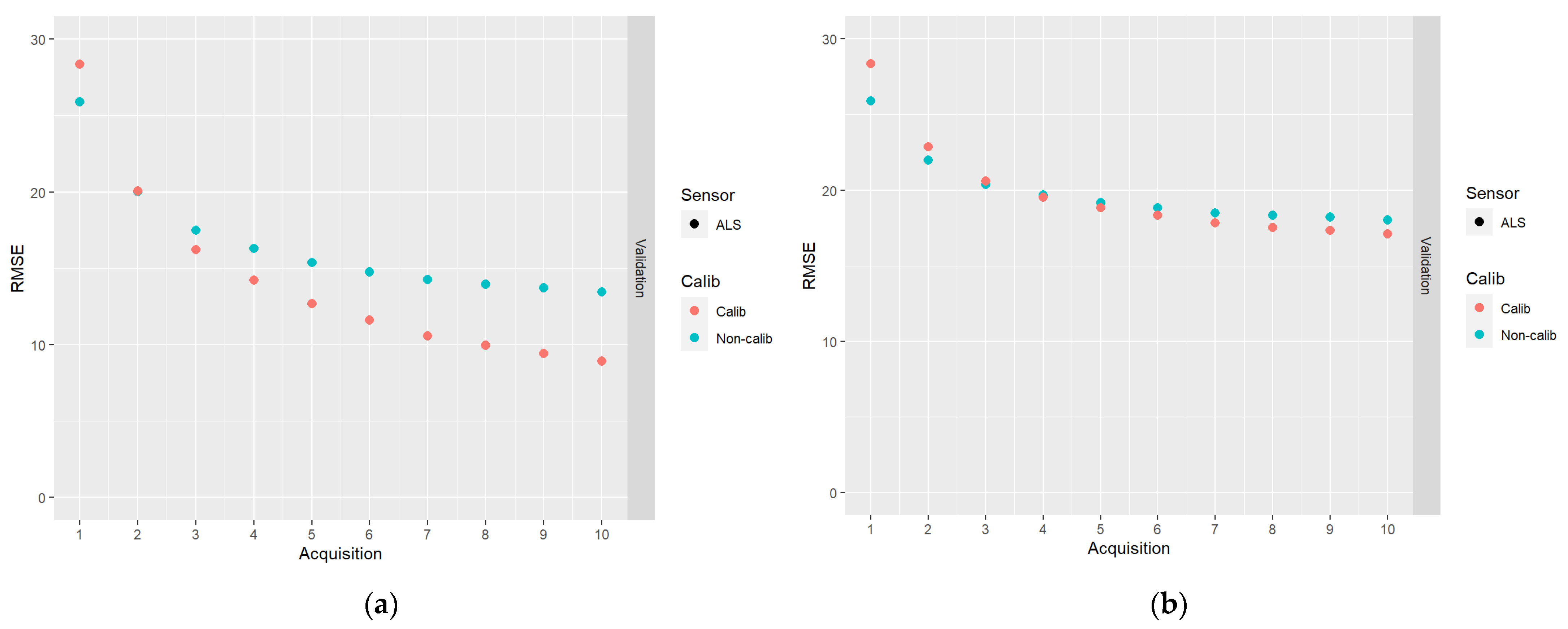
In Figure 6, results for the DA schemes based on 10 acquisitions of ALS data are shown.
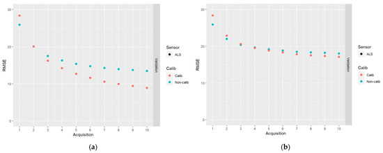
Figure 6.
The results of DA schemes applying a sequence of 10 acquisitions of ALS data: (a) no correlations between model errors were simulated (case I); (b) correlations were simulated according to Table 2 (case II).
From Figure 6, it can be seen that whereas the RMSEs initially increased due to the calibration, they decreased faster when predictions were calibrated compared to when they were not calibrated. Thus, at the end of the sequence of acquisitions, the RMSEs were smaller for the calibrated predictions compared to the non-calibrated predictions. This effect was stronger for the case of data simulated without plot level error correlations (case I). As could be observed in Figure 5, another advantage of calibrated predictions is that they are approximately unbiased.
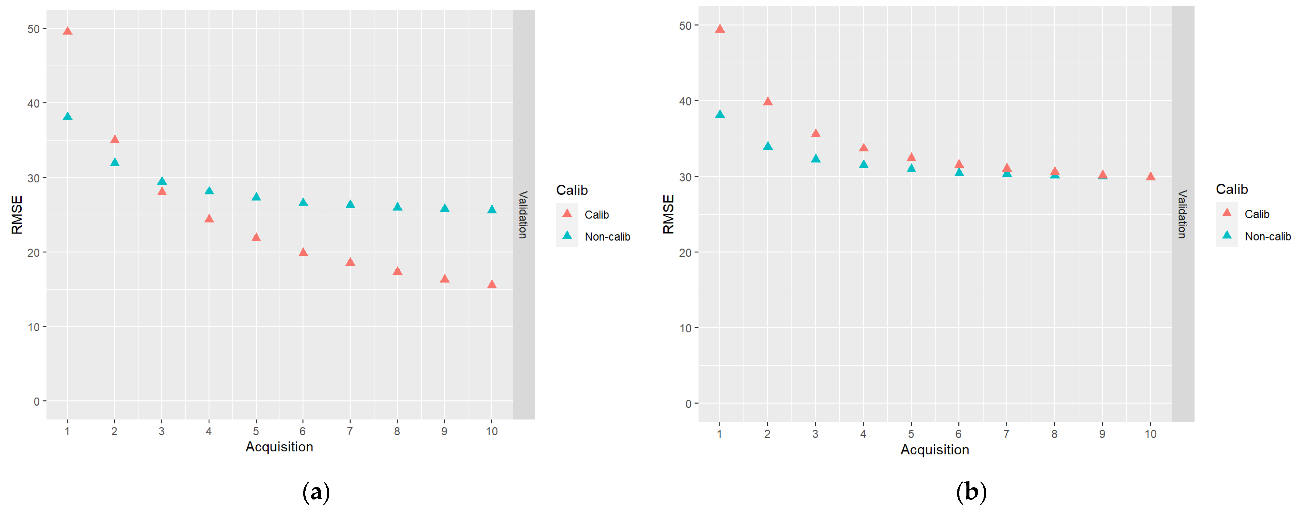
In Figure 7, results for the DA schemes based on 10 acquisitions of DP data are shown.
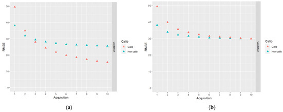
Figure 7.
The results of DA schemes applying a sequence of 10 acquisitions of DP data: (a) no correlations between model errors were simulated (case I); (b) correlations were simulated according to Table 2 (case II).
From Figure 7, the same general trends as in Figure 6 can be observed, i.e., the calibrated predictions initially have a larger RMSE and the decrease of the RMSE is faster than the non-calibrated predictions. In the case of DP predictions with simulated plot level error correlations, the endpoint RMSEs are about the same for calibrated and non-calibrated predictions. As for the ALS-based predictions, an advantage in the case of calibrated predictions is that they are approximately unbiased.
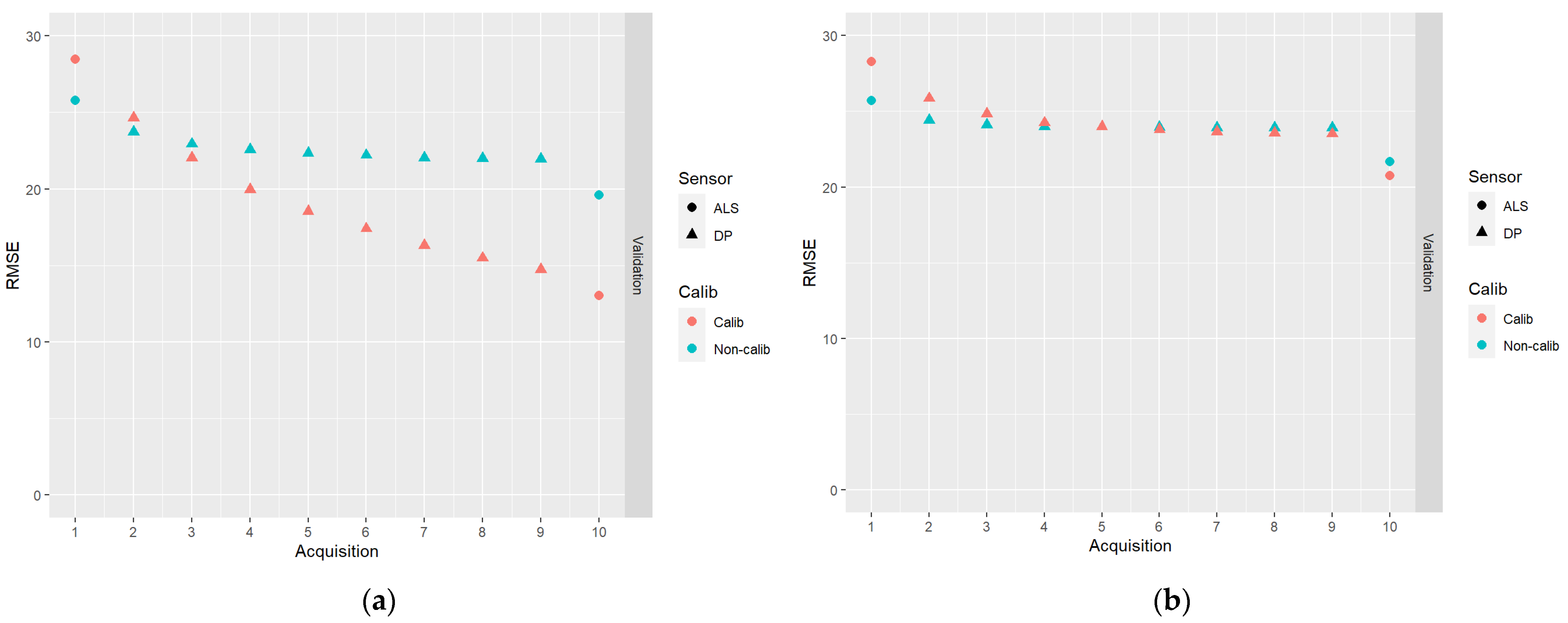
In Figure 8, results for the DA schemes based on the first acquisition of ALS data, followed by eight acquisitions of DP data, and ending with an ALS acquisition, are shown.
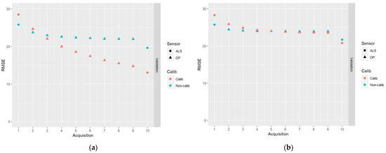
Figure 8.
The results of DA schemes based on the first acquisition of ALS data, followed by eight acquisitions of DP data, and ending with an ALS acquisition: (a) no correlations between model errors were simulated (case I); (b) correlations were simulated according to Table 2 (case II).
From Figure 8, it can be seen that predictions with poor accuracy (DP-based predictions in our study) can be successfully combined with accurate predictions (ALS-based in our study), especially in the case of calibrated predictions. It can be observed that the RMSEs of the endpoint predictions were only moderately larger than the RMSEs for the endpoint predictions using a full sequence of ALS-based predictions (Figure 6).
4. Discussion
This study emanated from the difference between the theoretical potential of DA in forestry, as demonstrated by [8], and the results from empirical studies obtained by [10] and [11]. While the first study indicated a substantial potential for DA to improve the precision of predictions, the latter two studies obtained only modest improvements for DA compared to using only the latest available prediction. A study by [12] suggested that correlated errors between successive predictions based on RS data could be an important reason for this. Different explanations for correlated errors were discussed (ibid.), and it was suggested that the tendency of RS-based estimates, following regression analysis and similar machine learning techniques, to be shrunk towards the mean value could be an important explanation (cf., [33]). This is a standard effect of regression analysis when variables that are poorly or moderately correlated with the dependent variable are applied as explanatory variables since regression analysis and similar machine learning techniques are designed to provide unbiased predictions conditional on the predictor variables, but not unbiased estimates conditional on the true values, i.e., the field reference values [25].
For efficient DA procedures, new observations or predictions need to be unbiased for each individual unit when DA is applied [28]. In this study, we suggest that classical calibration would be a means to achieve this, thus overcoming some of the problems identified in previous forest inventory studies. Our simulation results give strong support to this hypothesis, showing that calibration is especially important when assimilating predictions based on RS data that are only weakly correlated with the dependent variable. A study by Lindgren et al. [13], based on empirical data, also provided evidence that calibration improves the efficiency of DA in forest applications based on model predictions. The reason for this effect is that without calibration, a systematic deviation between the predicted value and the true value typically remains at the level of individual units regardless of the number of predictions added to the assimilation scheme. Since calibration removes this systematic deviation, the DA results improve, although the initial effect of calibration is increased RMSE. However, it should be noted that our results are based on simulations assuming a large number of observations available to fit and assess models. In practice, with small datasets, results would depend on data availability.
Alternatives to classical calibration exist, which might produce similar, although not identical results [27]. One such well-known calibration method is inverse calibration (e.g., [36]), the results of which could be worthwhile to investigate for the current application. Barth et al. [37] suggested an imputation-based calibration method where the composition of the calibrated plots was constrained to correspond to the composition of the plots in the reference dataset. Such an approach overcomes problems that might occur with other calibration methods, where some calibrated values could be negative. Thus, in practical applications, different calibration approaches might be needed for different parts of the dataset, or simple truncation be applied to avoid negative values.
If error correlations between predictions could be avoided, DA has a considerable potential to improve predictions of forest attributes at plot- and stand-level. In such a case, the standard deviation of the DA predictions would decrease by a factor , with n being the number of predictions included, provided that growth updates can be made accurately. In practice it is likely that several factors contribute to correlated errors. For example, special conditions on a sample plot with regard to foliage or topographic conditions might cause correlated errors, and it needs to be further investigated to what extent such conditions affect the correlations and, thus, the efficiency of DA procedures.
Although the proposed calibration method increased the RMSE when applied to predictions based on a single acquisition of RS data, it might be worthwhile to consider it also in connection with standard mapping and estimation based on RS data. For example, if RS-based estimates are severely shrunk towards the mean, the implications of using them in forest planning might be significant [37].
5. Conclusions
In this study, we have demonstrated that correlated model residual errors due to regression predictions being shrunk towards the mean make DA procedures less efficient. We have also shown that classical calibration is a means to overcome this problem, and our study suggests that classical calibration, in most cases, increased the accuracy of DA-based predictions when the growing stock volume was predicted at the level of plots. The study thus has the potential to contribute to implementing efficient DA schemes in practical forest inventories in the future. However, such schemes would need to take into account that the datasets available for model training and evaluation would mostly be much smaller than the ones available in this simulation study.
Author Contributions
Conceptualization, N.L., K.N., S.S., H.O. and G.S.; methodology, N.L., K.N., S.S., H.O. and G.S.; software, S.S.; validation, N.L., K.N., S.S., H.O. and G.S.; formal analysis, N.L. and S.S.; investigation, N.L., K.N., S.S., H.O. and G.S.; data curation, N.L. and S.S.; writing—original draft preparation, N.L. and G.S.; writing—review and editing, N.L., K.N., S.S., H.O. and G.S.; visualization, S.S.; supervision, H.O. and G.S.; project administration, H.O.; funding acquisition, H.O. and G.S. All authors have read and agreed to the published version of the manuscript.
Funding
This research was funded by the Swedish research council Formas (grant number 942-2015-63), by the Swedish University of Agricultural Science, and by the Research Council of Norway, project “SmartForest” (grant number 309671).
Institutional Review Board Statement
Not applicable.
Informed Consent Statement
Not applicable.
Data Availability Statement
Not applicable.
Acknowledgments
We thank three anonymous Reviewers for their comments, which helped us to improve the manuscript.
Conflicts of Interest
The authors declare no conflict of interest.
References
- Ghil, M.; Malanotte-Rizzoli, P. Data Assimilation in Meteorology and Oceanography. In Advances in Geophysics; Elsevier: Amsterdam, The Netherlands, 1991; Volume 33, pp. 141–266. ISBN 978-0-12-018833-8. [Google Scholar]
- Rabier, F. Overview of Global Data Assimilation Developments in Numerical Weather-Prediction Centres. Q. J. R. Meteorol. Soc. 2005, 131, 3215–3233. [Google Scholar] [CrossRef]
- Dowd, M. Bayesian Statistical Data Assimilation for Ecosystem Models Using Markov Chain Monte Carlo. J. Mar. Syst. 2007, 68, 439–456. [Google Scholar] [CrossRef]
- Dixon, B.L.; Howitt, R.E. Continuous Forest Inventory Using a Linear Filter. For. Sci. 1979, 25, 675–689. [Google Scholar] [CrossRef]
- Czaplewski, R.L.; Alig, R.J.; Cost, N.D. Monitoring Land/Forest Cover Using the Kalman Filter: A Proposal. In Ek, Alan R.; Shifley, Stephen R.; Burk, Thomas E. Forest Growth Modelling and Prediction: Volume 2. Gen. Tech. Report NC-120; US Deptartment of Agriculture, Forest Service, North Central Forest Experiment Station: St. Paul, MN, USA, 1988; pp. 1089–1096. [Google Scholar]
- Kangas, A. Updated Measurement Data as Prior Information in Forest Inventory. Silva Fenn. 1991, 25, 181–191. [Google Scholar] [CrossRef]
- Kalman, R.E. A New Approach to Linear Filtering and Prediction Problems. J. Basic Eng. 1960, 82, 35–45. [Google Scholar] [CrossRef]
- Ehlers, S.; Grafström, A.; Nyström, K.; Olsson, H.; Ståhl, G. Data Assimilation in Stand-Level Forest Inventories. Can. J. For. Res. 2013, 43, 1104–1113. [Google Scholar] [CrossRef]
- Saad, R.; Eyvindson, K.; Gong, P.; Lämås, T.; Ståhl, G. Potential of Using Data Assimilation to Support Forest Planning. Can. J. For. Res. 2017, 47, 690–695. [Google Scholar] [CrossRef]
- Nyström, M.; Lindgren, N.; Wallerman, J.; Grafström, A.; Muszta, A.; Nyström, K.; Bohlin, J.; Willén, E.; Fransson, J.; Ehlers, S.; et al. Data Assimilation in Forest Inventory: First Empirical Results. Forests 2015, 6, 4540–4557. [Google Scholar] [CrossRef]
- Lindgren, N.; Persson, H.J.; Nyström, M.; Nyström, K.; Grafström, A.; Muszta, A.; Willén, E.; Fransson, J.E.S.; Ståhl, G.; Olsson, H. Improved Prediction of Forest Variables Using Data Assimilation of Interferometric Synthetic Aperture Radar Data. Can. J. Remote Sens. 2017, 43, 374–383. [Google Scholar] [CrossRef]
- Ehlers, S.; Saarela, S.; Lindgren, N.; Lindberg, E.; Nyström, M.; Persson, H.; Olsson, H.; Ståhl, G. Assessing Error Correlations in Remote Sensing-Based Estimates of Forest Attributes for Improved Composite Estimation. Remote Sens. 2018, 10, 667. [Google Scholar] [CrossRef]
- Lindgren, N.; Olsson, H.; Nyström, K.; Nyström, M.; Ståhl, G. Data Assimilation of Growing Stock Volume Using a Sequence of Remote Sensing Data from Different Sensors. Can. J. Remote Sens. 2022, 48, 127–143. [Google Scholar] [CrossRef]
- Hou, Z.; Mehtätalo, L.; McRoberts, R.E.; Ståhl, G.; Tokola, T.; Rana, P.; Siipilehto, J.; Xu, Q. Remote Sensing-Assisted Data Assimilation and Simultaneous Inference for Forest Inventory. Remote Sens. Environ. 2019, 234, 111431. [Google Scholar] [CrossRef]
- Wallerman, J.; Holmgren, J. Estimating Field-Plot Data of Forest Stands Using Airborne Laser Scanning and SPOT HRG Data. Remote Sens. Environ. 2007, 110, 501–508. [Google Scholar] [CrossRef]
- Rahlf, J.; Breidenbach, J.; Solberg, S.; Næsset, E.; Astrup, R. Comparison of Four Types of 3D Data for Timber Volume Estimation. Remote Sens. Environ. 2014, 155, 325–333. [Google Scholar] [CrossRef]
- Yu, X.; Hyyppä, J.; Karjalainen, M.; Nurminen, K.; Karila, K.; Vastaranta, M.; Kankare, V.; Kaartinen, H.; Holopainen, M.; Honkavaara, E.; et al. Comparison of Laser and Stereo Optical, SAR and InSAR Point Clouds from Air- and Space-Borne Sources in the Retrieval of Forest Inventory Attributes. Remote Sens. 2015, 7, 15933–15954. [Google Scholar] [CrossRef]
- Tellinghuisen, J. Inverse vs. Classical Calibration for Small Data Sets. Fresenius J. Anal. Chem. 2000, 368, 585–588. [Google Scholar] [CrossRef] [PubMed]
- Persson, H.J.; Ståhl, G. Characterizing Uncertainty in Forest Remote Sensing Studies. Remote Sens. 2020, 12, 505. [Google Scholar] [CrossRef]
- Reese, H.; Nilsson, M.; Pahlén, T.G.; Hagner, O.; Joyce, S.; Tingelöf, U.; Egberth, M.; Olsson, H. Countrywide Estimates of Forest Variables Using Satellite Data and Field Data from the National Forest Inventory. AMBIO J. Hum. Environ. 2003, 32, 542–548. [Google Scholar] [CrossRef]
- Tomppo, E.; Olsson, H.; Ståhl, G.; Nilsson, M.; Hagner, O.; Katila, M. Combining National Forest Inventory Field Plots and Remote Sensing Data for Forest Databases. Remote Sens. Environ. 2008, 112, 1982–1999. [Google Scholar] [CrossRef]
- Næsset, E. Predicting Forest Stand Characteristics with Airborne Scanning Laser Using a Practical Two-Stage Procedure and Field Data. Remote Sens. Environ. 2002, 80, 88–99. [Google Scholar] [CrossRef]
- Næsset, E.; Gobakken, T.; Holmgren, J.; Hyyppä, H.; Hyyppä, J.; Maltamo, M.; Nilsson, M.; Olsson, H.; Persson, Å.; Söderman, U. Laser Scanning of Forest Resources: The Nordic Experience. Scand. J. For. Res. 2004, 19, 482–499. [Google Scholar] [CrossRef]
- Nilsson, M.; Nordkvist, K.; Jonzén, J.; Lindgren, N.; Axensten, P.; Wallerman, J.; Egberth, M.; Larsson, S.; Nilsson, L.; Eriksson, J.; et al. A Nationwide Forest Attribute Map of Sweden Predicted Using Airborne Laser Scanning Data and Field Data from the National Forest Inventory. Remote Sens. Environ. 2017, 194, 447–454. [Google Scholar] [CrossRef]
- Weisberg, S. Applied Linear Regression; John Wiley & Sons: Hoboken, NJ, USA, 2005; Volume 528, ISBN 0-471-70408-3. [Google Scholar]
- Eisenhart, C. The Interpretation of Certain Regression Methods and Their Use in Biological and Industrial Research. Ann. Math. Stat. 1939, 10, 162–186. [Google Scholar] [CrossRef]
- Osborne, C. Statistical Calibration: A Review. Int. Stat. Rev. Rev. Int. Stat. 1991, 59, 309. [Google Scholar] [CrossRef]
- Fridman, J.; Holm, S.; Nilsson, M.; Nilsson, P.; Ringvall, A.; Ståhl, G. Adapting National Forest Inventories to Changing Requirements—The Case of the Swedish National Forest Inventory at the Turn of the 20th Century. Silva Fenn. 2014, 48, 1095. [Google Scholar] [CrossRef]
- Chen, Q.; McRoberts, R.E.; Wang, C.; Radtke, P.J. Forest Aboveground Biomass Mapping and Estimation across Multiple Spatial Scales Using Model-Based Inference. Remote Sens. Environ. 2016, 184, 350–360. [Google Scholar] [CrossRef]
- Boucher, A.; Dimitrakopoulos, R. Block Simulation of Multiple Correlated Variables. Math. Geosci. 2009, 41, 215–237. [Google Scholar] [CrossRef]
- R Core Team. R: A Language and Environment for Statistical Computing; R Foundation for Statistical Computing: Vienna, Austria, 2022; Available online: https://www.R-project.org/ (accessed on 3 September 2022).
- Tian, Y.; Nearing, G.S.; Peters-Lidard, C.D.; Harrison, K.W.; Tang, L. Performance Metrics, Error Modeling, and Uncertainty Quantification. Mon. Weather Rev. 2016, 144, 607–613. [Google Scholar] [CrossRef]
- Hibbert, D.B.; Gooding, J.J. Data Analysis for Chemistry: An Introductory Guide for Students and Laboratory Scientists; Oxford University Press: New York, NY, USA, 2006; ISBN 0-19-516210-2. [Google Scholar]
- Grafström, A.; Ekström, M.; Jonsson, B.G.; Esseen, P.-A.; Ståhl, G. On Combining Independent Probability Samples. Surv. Methodol. 2019, 45, 349–364. [Google Scholar]
- Saarela, S.; Grafström, A. DatAssim: Data Assimilation; R Package Version 1.0. 2017. Available online: https://cran.r-project.org/package=DatAssim (accessed on 3 September 2022).
- Krutchkoff, R.G. Classical and Inverse Regression Methods of Calibration. Technometrics 1967, 9, 425–439. [Google Scholar] [CrossRef]
- Barth, A.; Lind, T.; Ståhl, G. Restricted Imputation for Improving Spatial Consistency in Landscape Level Data for Forest Scenario Analysis. For. Ecol. Manag. 2012, 272, 61–68. [Google Scholar] [CrossRef]
Publisher’s Note: MDPI stays neutral with regard to jurisdictional claims in published maps and institutional affiliations. |
© 2022 by the authors. Licensee MDPI, Basel, Switzerland. This article is an open access article distributed under the terms and conditions of the Creative Commons Attribution (CC BY) license (https://creativecommons.org/licenses/by/4.0/).

