Article

Spatiotemporal Variation, Driving Mechanism and Predictive Study of Total Column Ozone: A Case Study in the Yangtze River Delta Urban Agglomerations

1
School of Surveying and Land Information Engineering, Henan Polytechnic University, Jiaozuo 454000, China
2
South China Institute of Environmental Science, Ministry of Ecology and Environment, Guangzhou 510535, China
3
National Key Laboratory of Urban Ecological Environment Simulation and Protection, Guangzhou 510535, China
4
Guangzhou Urban Renewal Planning Institute, Guangzhou 510030, China
*
Author to whom correspondence should be addressed.
Remote Sens. 2022, 14(18), 4576; https://doi.org/10.3390/rs14184576
Submission received: 14 July 2022 / Revised: 17 August 2022 / Accepted: 5 September 2022 / Published: 13 September 2022

Abstract

:
Total column ozone (TCO) describes the amount of ozone in the entire atmosphere. Many scholars have used the lower resolution data to study TCO in different regions, but new phenomena can be discovered using high-precision and high-resolution TCO data. This paper used the long time, high accuracy, and high-resolution MSR2 dataset (2000–2019) to analyze the spatial and temporal variation characteristics of TCO over the Yangtze River Delta Urban Agglomeration to explore the relationship between the TCO and meteorological and socio-economic factors. The correlations between the TCO and climatic factors and the driving forces of meteorological and socio-economic factors on the spatial and temporal variability of TCO were also analyzed, and different mathematical models were constructed to fit the TCO for the past 20 years and predict the future trend of the TCO. The results show the following. (1) The TCO over the study area exhibited a quasi-latitudinal distribution, following a slight downtrend during 2000–2019 (0.01 ± 0.18 DU per year) and achieved its maximum in 2010 and minimum in 2019; throughout the year, an inverted V-shaped cycle characterizes the monthly variability of TCO; TCO was significantly higher in spring than in summer and autumn than winter. (2) Precipitation and the absorbed aerosol index (AAI) had critical effects on the spatial distribution of TCO, but meteorological factors were weakly correlated with the annual variation of TCO subject to the game interactions between different external driving factors. The monthly changes in the TCO were not in synergy with that of other meteorological factors, but with a significant hysteresis effect by 3–5 months. Socio-economic factors had a significant influence on TCO over the study area. (3) The Fourier function model can well describe the history and future trend of the annual TCO over the study area. The TCO over the study area shows a fluctuating upward trend (0.27 ± 1.35 DU per year) over the next 11 years. This study enriches the theoretical and technical system of ozone research, and its results can provide the necessary theoretical basis for ozone simulation and forecasting.

1. Introduction

Ozone (O3), also called super oxygen, is a light blue gas with a special odor at normal temperature. O3 is an essential trace gas in the atmosphere that keeps the Earth’s living things from being exposed to excess ultraviolet radiation by blocking the vast majority of the ultraviolet radiation from the Sun, thereby maintaining normal survival and reproduction for living beings [1]. O3 is also one of the greenhouse gases. The O3 in the stratosphere can absorb a large amount of the Earth’s long-wave radiation to increase the temperature of the low-level atmosphere, and it has an important effect on the atmospheric circulation and temperature field [2]. However, over the ground level, superhigh concentration O3 is considered as a harmful pollutive gas since it can damage the human respiratory system to a certain degree [3] and cause a reduction in the crop yield and damage in vegetation growth [4]. Over recent years, with the fast development of China’s economy and continuous advance in urbanization development, the concentration of O3 over the perigee surface has kept increasing to the point that O3 has evolved gradually as one of the most important air pollutants following the fine particulate matter (PM2.5) [5]. The frequent incidence of O3 pollution has severely damaged the human living environment and posed a huge barrier to social and economic development. Therefore, it has become increasingly important to monitor and study the O3 in the atmosphere.
The total column ozone (TCO) is the total amount of O3 in a column extending vertically from the Earth’s surface to the top of the atmosphere. It is measured using ground-based stations and satellites and is reported in Dobson units (DU). The continuous development in remote sensing technology has made it possible to monitor the TCO in a long-time sequence and continuous space. The emerging TCO products have played an increasingly important role in O3-related studies. For example, quite a few scholars have utilized satellite remote sensing based TCO products to study the ozonosphere hole and its repair [6,7,8]. Additionally, quite a few scholars have kept trying new methods for the inversion of TCO to obtain products with a higher accuracy and higher spatiotemporal resolution [9,10,11,12,13,14]. Under the support of these gradually superior and rich TCO products, the spatiotemporal variation characteristics and the influencing factors’ forcing mechanisms of O3 have also been more thoroughly revealed by scholars [15,16,17,18].
As an important factor representing the atmospheric concentration and distribution of O3 over an area, TCO has been used by many scholars to capture the pollution status of atmospheric O3 [19]. For example, J. Fishman et al. (1987) pointed out that measurements of the TCO from a space platform can be used to study the widespread O3 pollution episode over the southeastern United States [20]. A few years later, J. Fishman et al. (2017) further applied an empirically corrected technique on the TCO observations from a total ozone mapping spectrometer (TOMS) and stratospheric O3 profiles from the solar backscattered ultraviolet (SUBV) to obtain the global distribution of tropospheric O3 and further identified the regional O3 pollution in Northeastern India, Eastern United States, Eastern China, and West and Southern Africa [21]. Azmi, Awang, and Ya’Acob [19] studied the coordinated variations of ground level O3 and the TCO concentrations over Klang Valley, Malaysia in 2014 and 2015, and the results showed that the ground level ozone exhibited observable peaks at the same period as the TCO. To summarize the previous research, it can be found that there remain considerable blanks in exploring the mechanisms behind the regional spatiotemporal variations of TCO, and that little is known about the time-lag effects of climatic factors in the TCO changes; furthermore, few attempts have been made to predict the future TCO variations.
The Yangtze River Delta area is one of the most economically developed areas in China, one with oversized urban agglomerations featuring a developed economy, great urban density, and crowded population and industrial activities in China. Contributing one quarter of China’s economic aggregate and above one quarter of the industrial added value, it is deemed as an important engine for China’s economic development. With the rapid economic development over recent years, the concentration in the precursors NOx and VOCs to O3 and of other atmospheric pollutants has kept increasing over the Yangtze River Delta, and O3 pollution has become increasingly severe to the point that top priority has to be given to the research on O3 pollution targeting this area. As far as the current status of research is concerned on the TCO distribution across China, most studies have utilized the TOMS and Ozone Monitoring Instrument (OMI) satellite data about O3 in the relatively early years, whose spatial resolution were relatively low [22]. Furthermore, so far, few studies have targeted the Yangtze River Delta, leaving a considerable gap of research on the spatiotemporal variation in the local O3 and its driving factors and mechanisms [23]. High-precision and high-resolution TCO data enable a more detailed study of different regions to discover other phenomena. In addition, though there have been a few studies on correlation analysis with the TCO using numerous meteorological and socioeconomic factors, research in the Yangtze River Delta is also essential. It is also noteworthy that studying the TCO spatial and temporal variation and prediction can provide significant reference values for regional environmental studies.
To fill the research gap, this paper used the Yangtze River Delta urban agglomeration as a case-study area, adopting the TCO data of a high-resolution, high-accuracy, multi-sensor reanalysis to study the spatiotemporal variation characteristics of the TCO over the study area over the last 20 years. Furthermore, the driving factors behind the spatiotemporal variation in the TCO are also discussed. Finally, a prediction was made about the TCO variation over this area in the upcoming 11 years on the basis of the historical data. This paper provides the essential scientific basis and decision-making references for environmental protection administrations of the Yangtze River Delta with respect to the governance of the atmospheric total ozone and environmental protection policymaking.

2. Material and Methods

2.1. The Studied Area

The Yangtze River Delta Urban Agglomerations are located in the alluvial plain formed before the estuary of the Yangtze River. It consists of 26 prefecture-level cities within the geographical range 28°01′–34°48′N, 115°46′–123°25′E, covering an area of 211.7 thousand km2. This area belongs to the subtropic monsoon climate type, with a mean annual precipitation between 84 mm and 123 mm and an annual average temperature between 15 °C and 17 °C.

2.2. Data

The O3 data adopted in this paper were the global TCO data of the global multisensor reanalysis (MSR2) (http://www.temis.nl/protocols/O3global.html, last access: 19 May 2022). It is a long-time sequence, high-accuracy, high-resolution O3 product [10]. They are reported in DU (Dobson unit), with a spatial resolution of 0.5°, and a temporal resolution of month. The reliability and accuracy of this dataset have been well-confirmed in previous studies on the spatiotemporal variation of TCO over different areas of the globe [24,25].
The meteorological data (i.e., air temperature, precipitation, and vapor pressure applied) stem from the widely used and accepted climate dataset (CRU TS v. 4.05) [26]. The absorbing aerosol index (AAI) used here integrated the products derived from the reflectance measured by GOME-1, SCIAMACHY, GOME-2, and OMI [27,28]. The data of the total solar radiation are the sum of down-going long-wave radiation and short-wave radiation that originated from Princeton University [29]. The social data including population, regional GDP, and proportions of primary, secondary, and tertiary industries were gathered from the China City Statistical Yearbook. These data were mainly used to analyze the driving forces on the TCO variation.

2.3. Methods

2.3.1. Correlation Analyses

Pearson’s correlation coefficient (R) was applied to analyze the correlations between the TOC and climatic (or economic) factors. The value of R statistically ranges from −1 to +1, wherein the negative (positive) values denote the negative (positive) correlations and the value of 0 represents no linear correlation.
R x y = i = 1 n x i x ¯ y i y ¯ i = 1 n ( x i x ¯ ) 2 i = 1 n y i y ¯ 2
where x and y are the TOC and climatic (or economic) factors, respectively.

2.3.2. Time-Lag Effects Analyses

In this study, the time-lag effects analyses were carried out through the following steps to obtain the lagged time intervals of the climatic factors on the TOC variations. First, it was assumed that certain lagged intervals (0 ≤ kn months) were exhibited in the effects of the climatic factors on TOC variations; then, at each supposed time lag, the accompanying R values (R0, R1, …, and Rn) between the climatic factors on TOC were obtained; finally, the R (Rk, 0 ≤ kn) with its maximum determination coefficient ( R k 2 ) was taken as the optimal R (OR, Equation (2)), where k is considered as the optimal time lag (OTL, Equation (3)) for the TOC responses to the variations in climatic factors.
OR   = R k ,   when   R k 2 =   Max R 0 2 , R 1 2 , , R n 2 0 k n
OL   =   k ,   when   R k 2 =   Max R 0 2 , R 1 2 , , R n 2 0 k n

2.3.3. Predictive Studies on TOC

This paper predicts the future TCO over the study area based on the historical data from 2000 to 2019. Three functions (i.e., the polynomial function, trigonometric function and Fourier function) are selected for the fitting of the TCO variation during 2000–2019. Then, the mathematical statistical parameters (i.e., R2, SSE, and RMSE) were calculated to compare the capacities of these fitting functions. Finally, the best fitting function was selected to predict the future TCO over the study area for the period of 2020–2030.

3. Results

3.1. Spatio-Temporal Variations of TCO over the Yangtze River Delta Urban Agglomerations

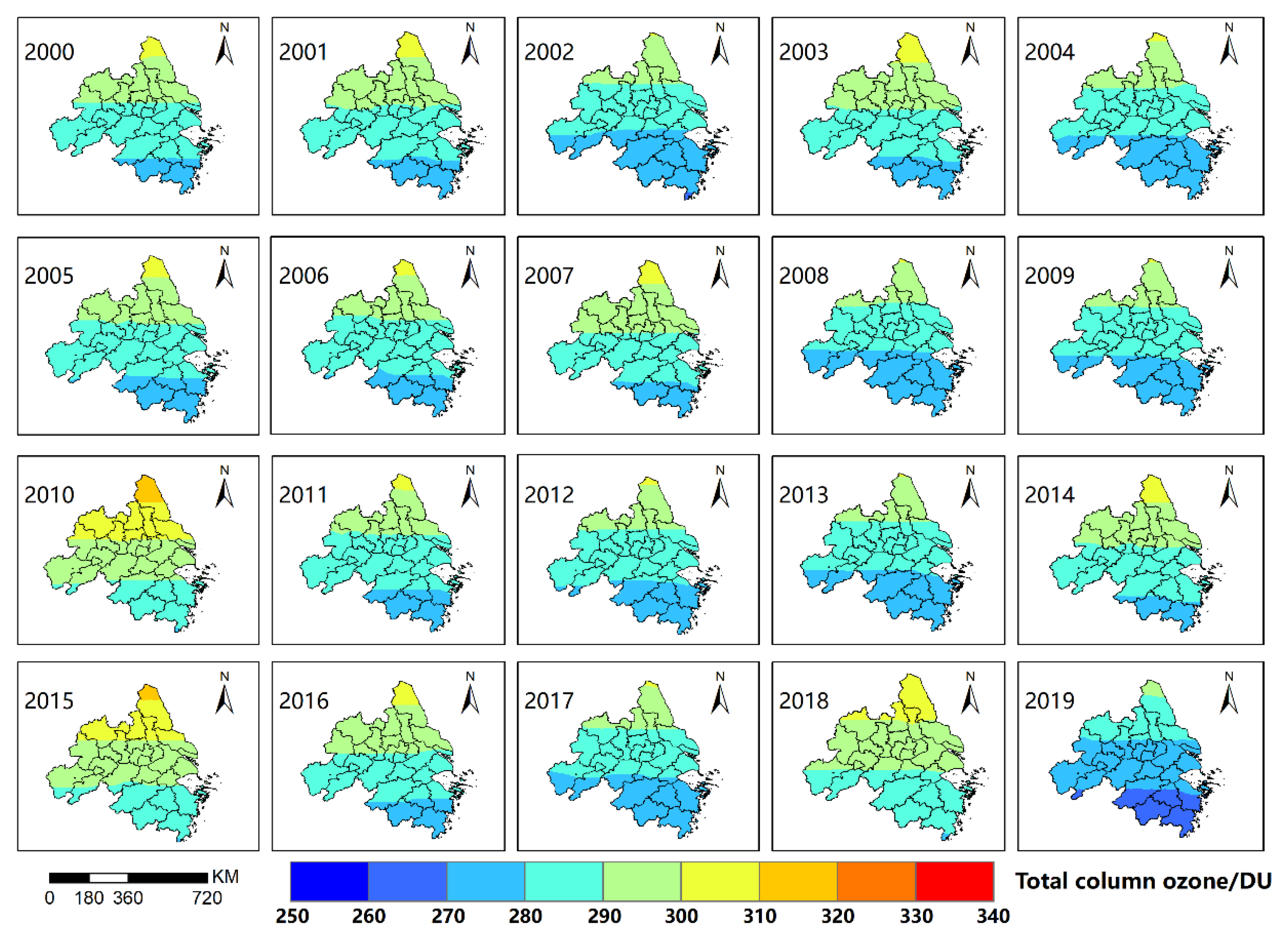
From Figure 1, the annual average TCO over the Yangtze River Delta Urban Agglomerations ranged between 270 DU and 310 DU during the past 20 years, with an average value of 286 DU, a minimum in Taizhou City, and a maximum in Yancheng City. The TCO exhibited a continuous quasi-latitudinal spatial distribution trend over the Yangtze River Delta Urban Agglomerations. However, certain differences existed in the TCO between different years (Appendix A, Figure A1). Obvious high-value intervals appeared in 2010, 2015, and 2018 compared to other years, mainly distributed in Yancheng City and a small part of areas in the nearby cities, while obvious low-value intervals appeared in 2002, 2008, and 2019, mainly distributed in the neighborhood around Jinhua City and Taizhou City.
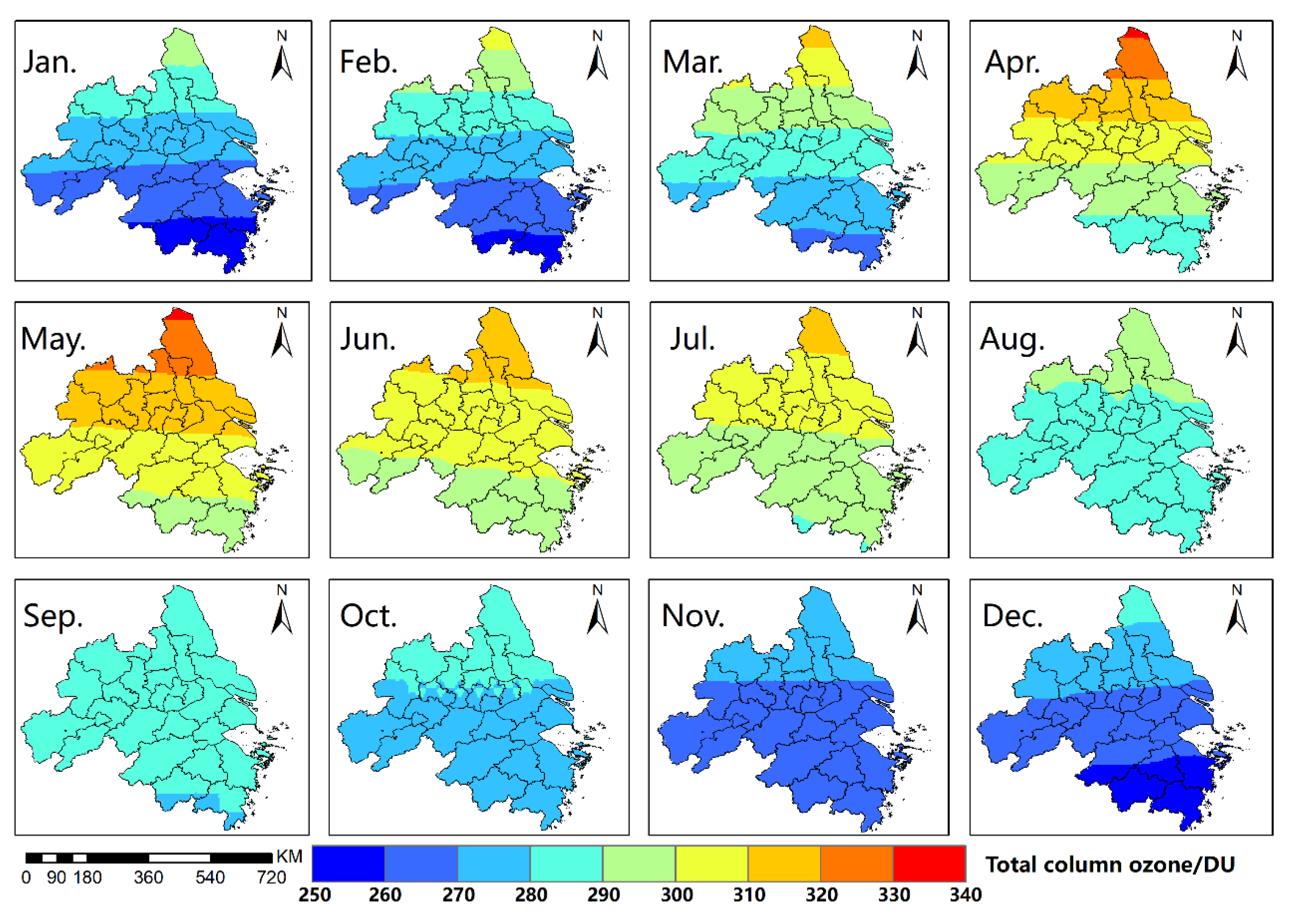
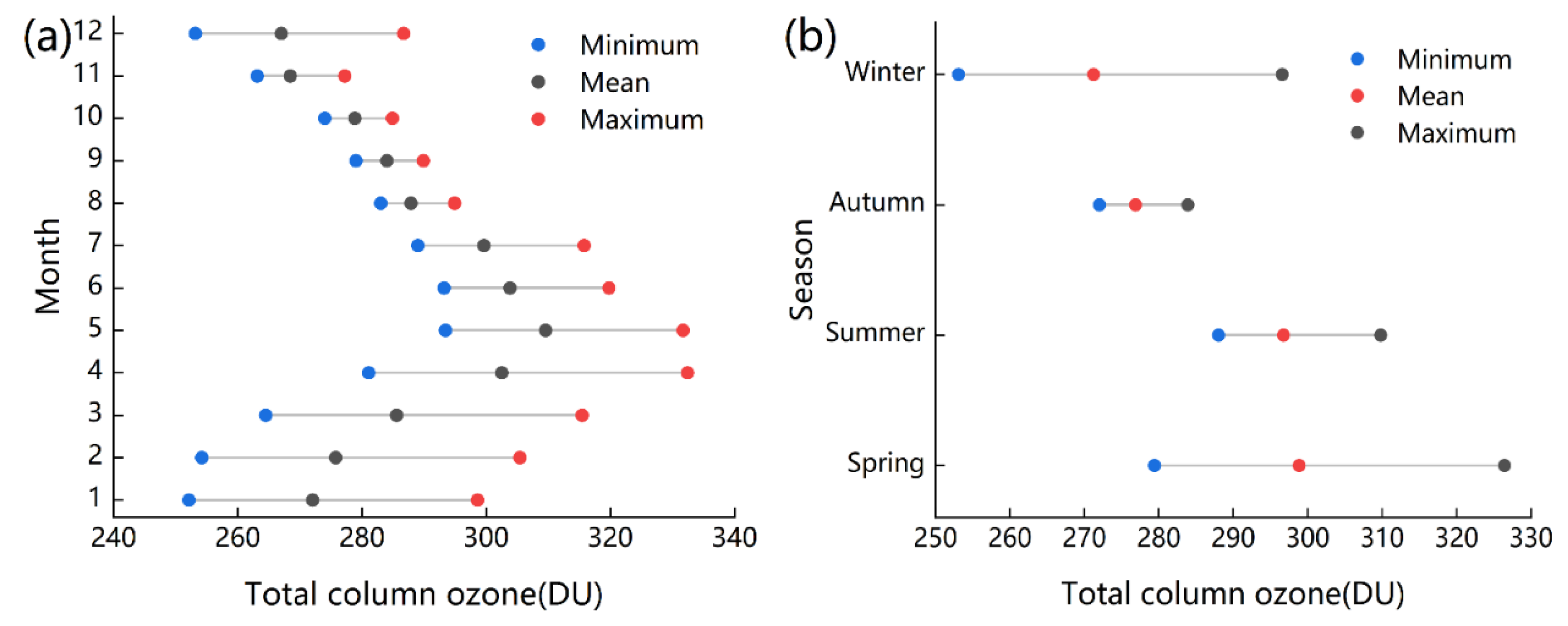
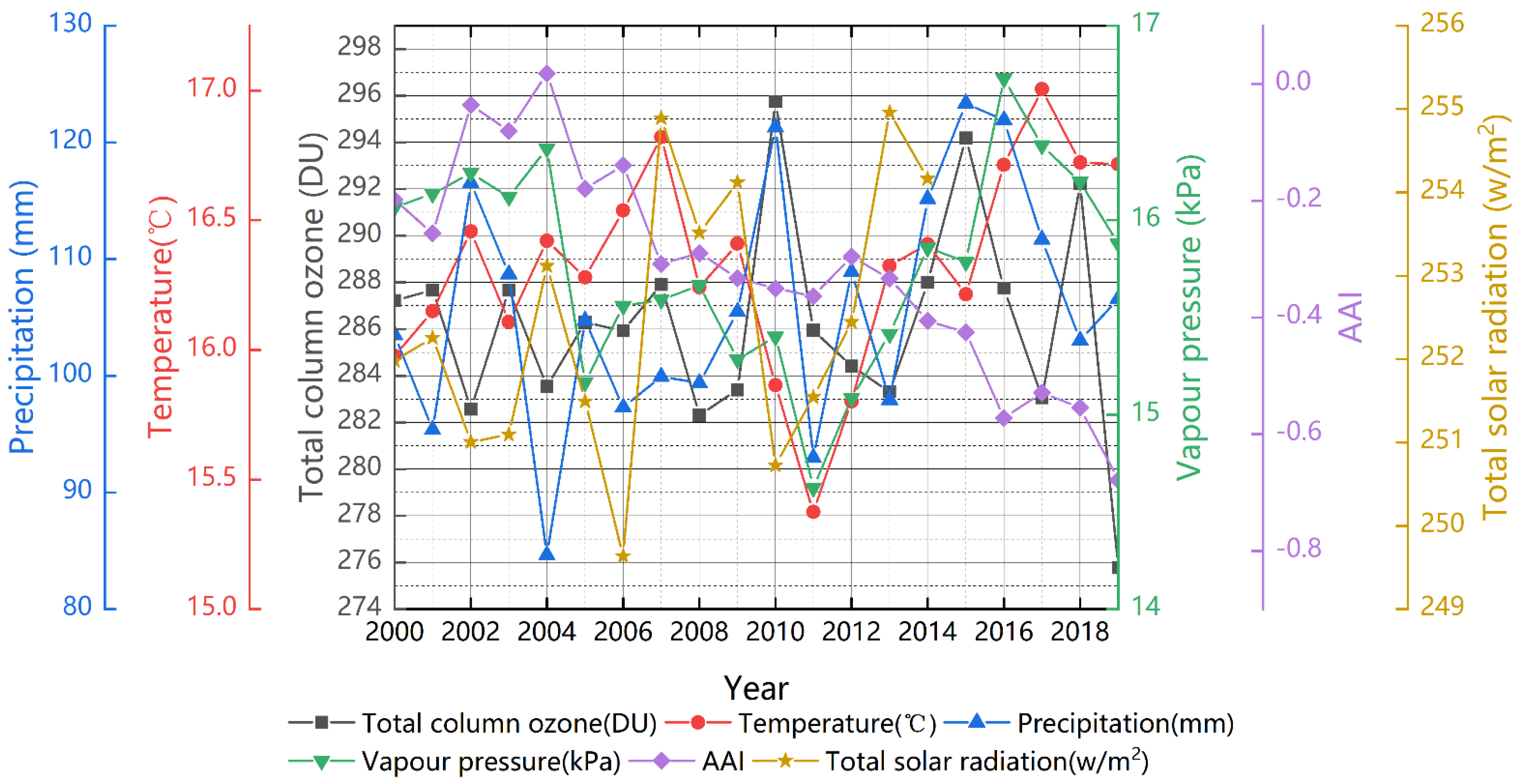
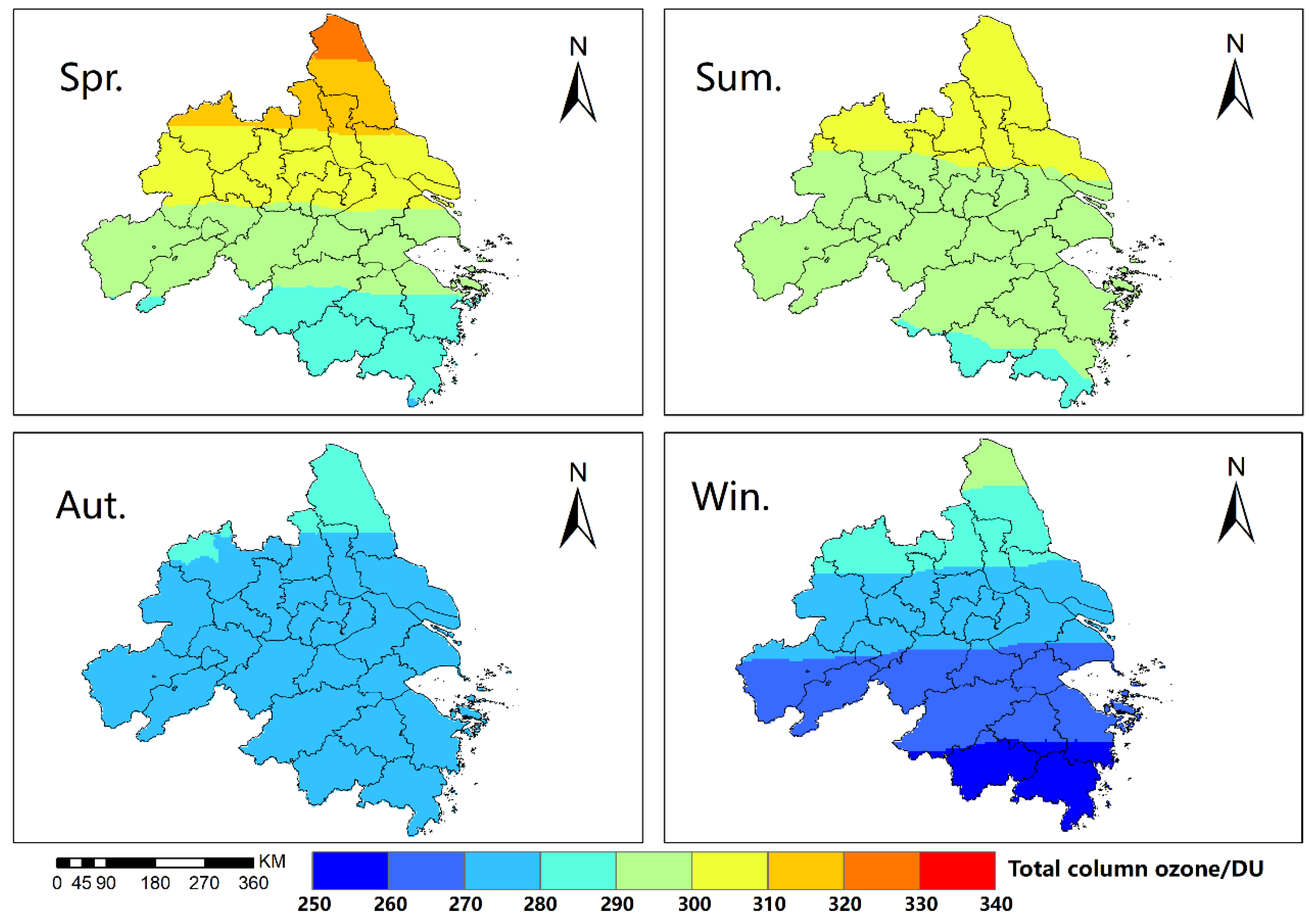
According to the annual variation curve of the mean of the TCO (Figure 2), the amplitude of the TCO variation over the study area was relatively steady during 2000–2009, after which the TCO rendered significant fluctuations; during the 20 years, the TCO over the Yangtze River Delta Urban Agglomerations dropped at a rate of −0.01 ± 0.18 DU per year, with the maximum of 295 DU in 2010 and the minimum of 275 DU in 2019 (a difference of 20 DU). From the TCO changes at the monthly scale in a year (Figure A2 and Figure A3), we can see that during January–May, the distribution of high-value intervals of the TCO rendered a gradually increasing trend, followed by a gradually decreasing trend afterward. The maxima of TCO occurred in April and May, whereas the minima occurred in January and December, which coincided with the preceding description regarding seasonal variation [30]. It can be seen from Figure 3 that the TCO over the Yangtze River Delta Urban Agglomerations was significantly higher in spring and summer than in autumn and winter; the spatially averaged TCO for the four seasons were 298 DU, 296 DU, 276 DU, and 271 DU [31].

3.2. TCO and Meteorological Factors Analysis

3.2.1. Analysis of Overall and Interannual Variability of TCO and Meteorological Factors

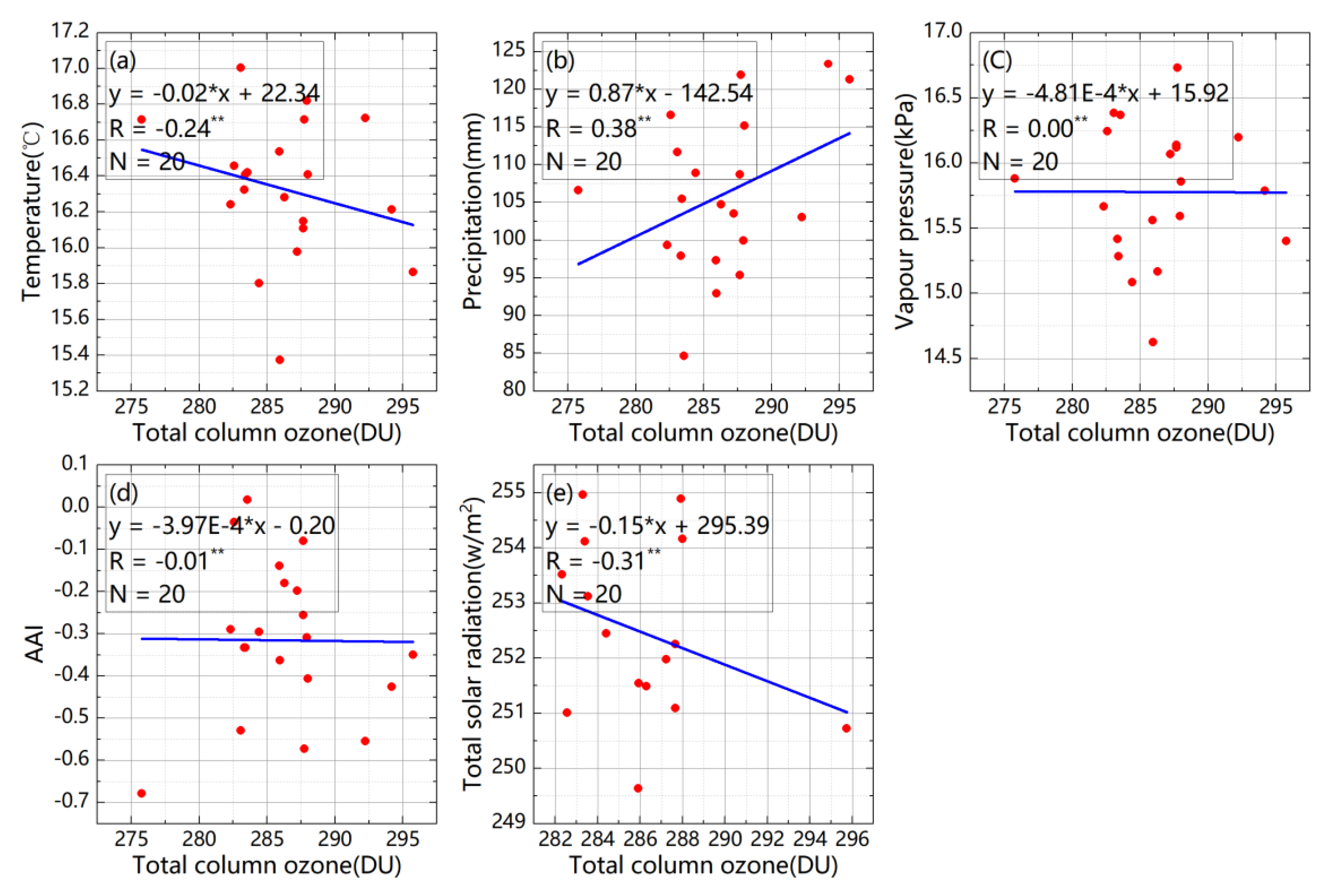
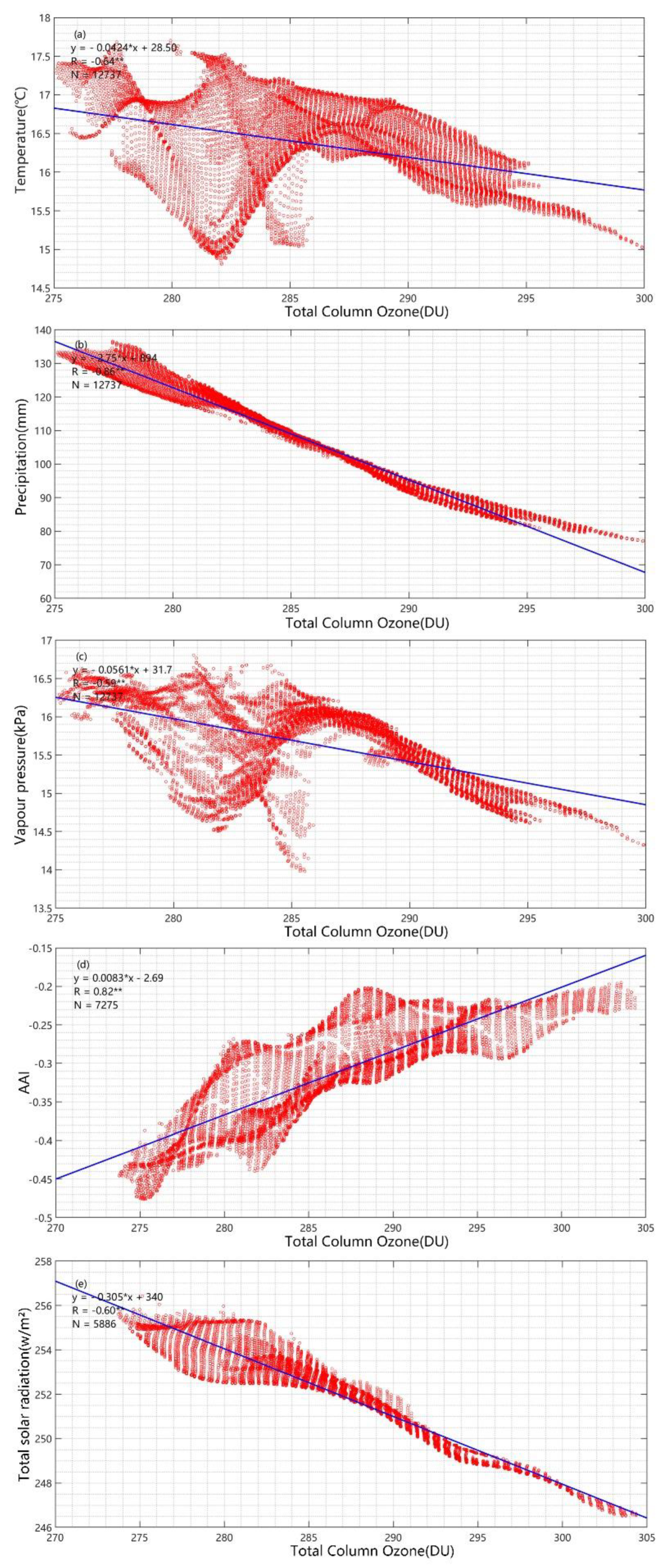
To investigate the relationship between the TCO and meteorological factors, we conducted a correlation analysis of the TCO and meteorological factors in time and space (Table 1, Figure A4 and Figure A5). For the space correlations (Table 1), there was a strong negative correlation between the TCO and precipitation, indicating that the decrease in the TCO in this area was mainly influenced by precipitation. There is a strong positive correlation between the TCO and AAI, indicating that the TCO is inextricably linked to the increase in the AAI. The correlation between the TCO and other meteorological factors was slightly weaker than this precipitation and the AAI. According to the results of the time correlations (Table 1), the TCO had a weak positive correlation to precipitation (R = 0.38) and a weak negative correlation to solar radiation (R = −0.31), and very weak correlations to all of the other meteorological factors. Furthermore, combining Figure 1a and Figure 4, it can be found that TCO had a similar quasi-latitudinal spatial distribution trend to precipitation and AAI, which further verified the significant influences of precipitation and AAI on the TCO in spatial variation.

3.2.2. Analysis of Inter-Monthly and Seasonal Variation of TCO and Meteorological Factors

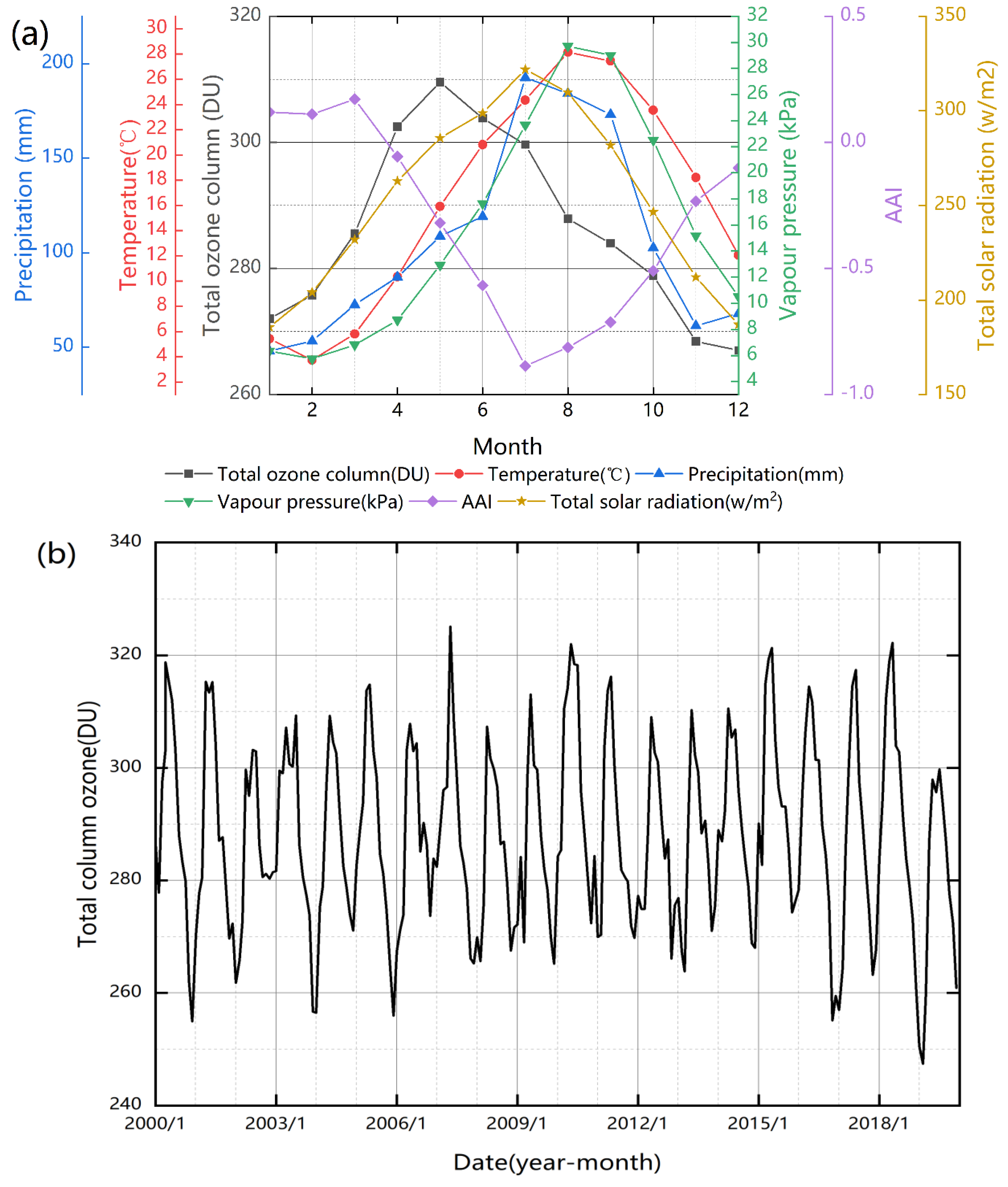
From Figure 5, the TCO, air temperature, precipitation, vapor pressure, and solar radiation presented obvious inverted V-shape time–sequence variation trends within a year. Furthermore, it was found that the TCO reached its maximum (309.55 DU, Figure 5, Table A1) in May, while the month for the maximum of these meteorological factors was not the same as the TCO. The AAI reached its annual minimum in July, presenting a V-shape time–sequence variation trend. From these results, we can see that there may exist a certain time lag between the changes in the TCO and climatic factors.
Based on the month-by-month data during 2000–2019, this paper further obtained the hysteretic response relation in the monthly variations between TCO and all of the meteorological factors. The results (Table 2) showed that the TCO had a three-month delayed response to air temperature and vapor pressure, a four-month delayed response to precipitation and AAI, and a five-month delayed response to solar radiation. These findings may provide important support and basis for the modeling, trend analyses, and future prediction of the TCO.

3.3. Correlation Analysis between TCO and Socioeconomic Factors

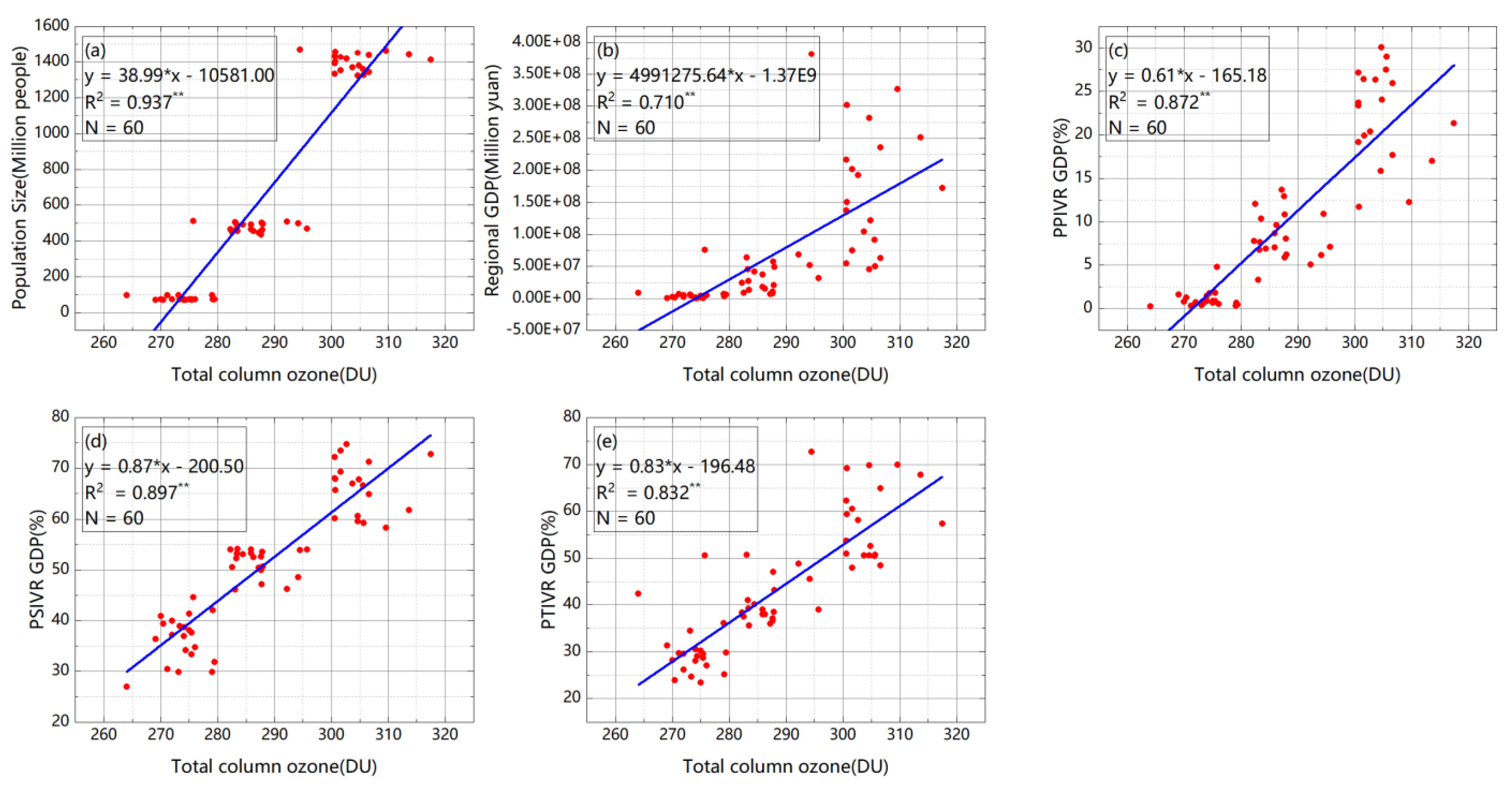
Population size, regional GDP, and the proportions of primary, secondary, and tertiary industries can reflect the economic development level of an area, which can further influence the changes in O3 [32]. From Table 3, TCO has the strongest correlation with population size. In addition, we found that the ratio value of the three industries had high positive correlations with the TCO, which was highest in the ratio value of secondary industry. These results might indicate that the TCO in the study area is closely and mainly influenced by the population size and the ratio value of the secondary industry there [33].

3.4. Predictive Analysis on TCO over the Yangtze River Delta Urban Agglomerations

3.4.1. Comparisons of the Fitting Functions of Historical TCO in the Yangtze River Delta Urban Agglomerations

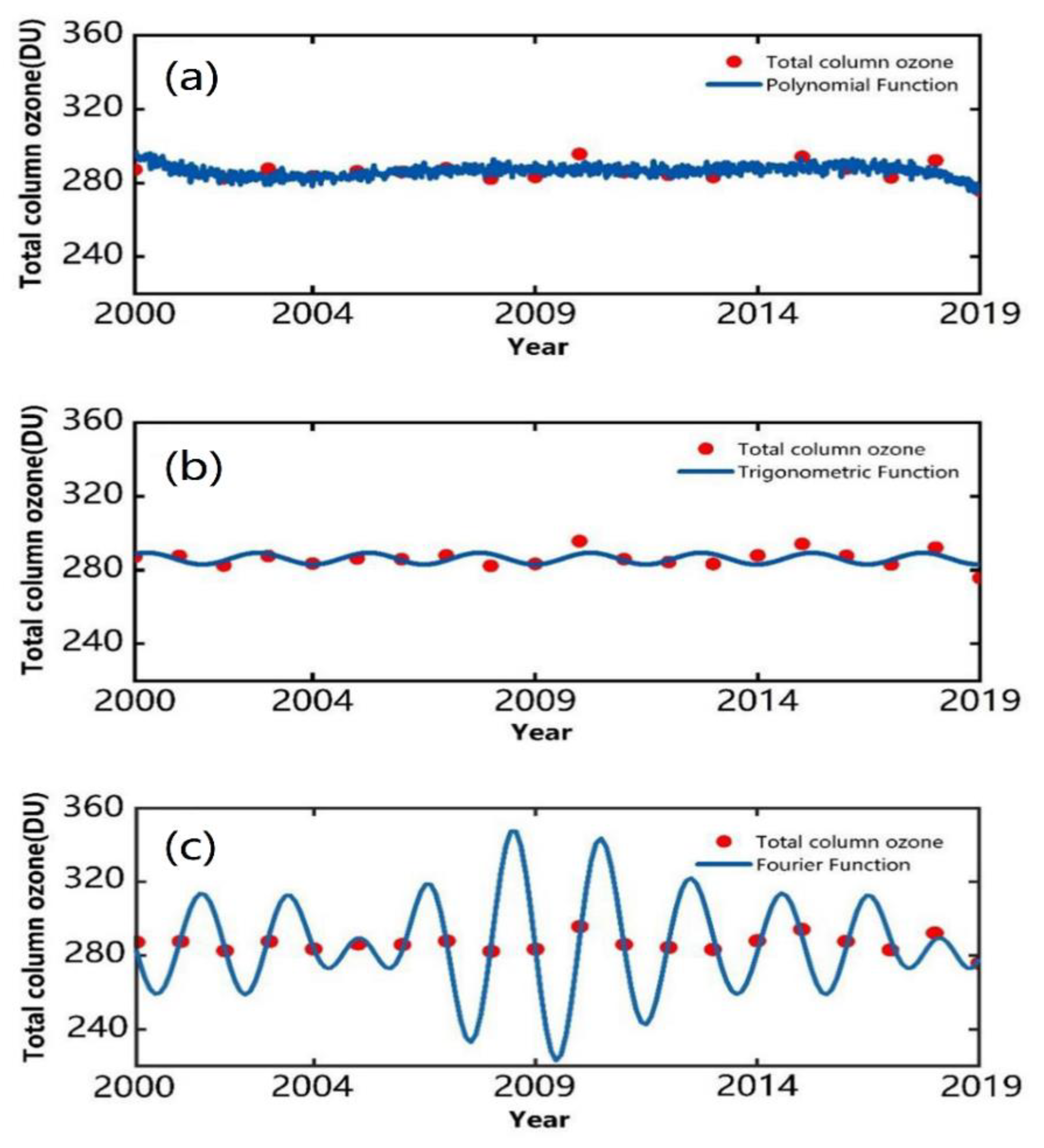
One linear function and two periodic functions were constructed to fit the annual TCO variations during 2000–2019 (Table 4). The results showed that the polynomial function was better fitted to the linear function. In addition, the Fourier function performed much better than the trigonometric function for the two polynomial functions. The fitting line charts of the three constructed functions for the historical TCO during 2000–2019 over the study area are shown in Figure 6. It can be found that the red points for the historical TCO fit very well with the fitting line of the Fourier function (Figure 6c), but not so well or badly with the fitting lines of the other two functions (Figure 6a,b). Furthermore, the accuracy analyses (Table 4) showed that the Fourier function was the best fitting function among the three functions constructed in this study, and it well depicted the annual TCO variations over the study area.

3.4.2. Analysis on the Prediction Results of Future TCO in the Yangtze River Delta Urban Agglomeration

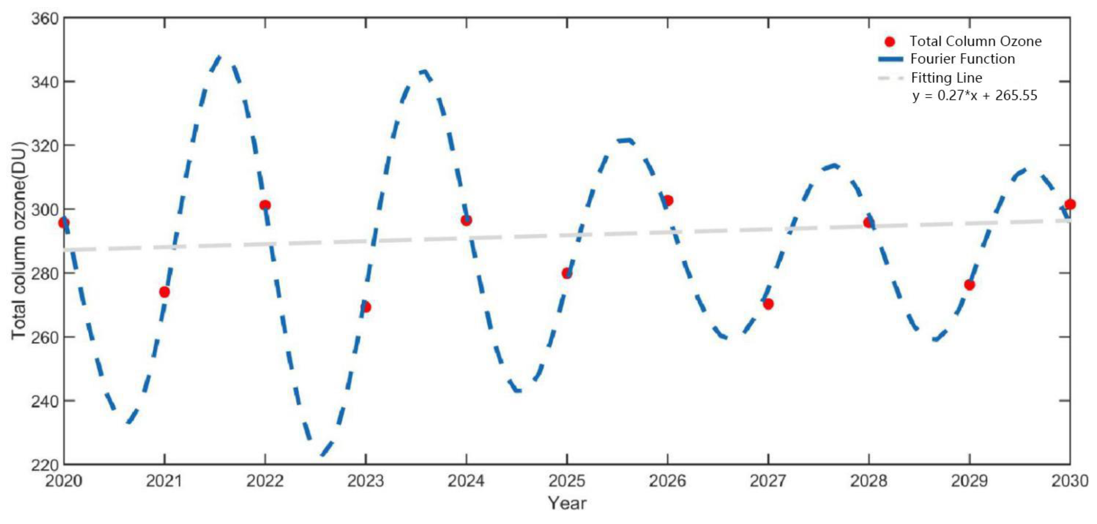
For the aforementioned reasons, the constructed Fourier function was utilized to predict the TCO over the study area during 2020–2030 (Figure 7 and Figure A8). The chart shows that the TCO over the Yangtze River Delta Urban Agglomerations rendered a fluctuating trend during this period, while the TCO overall rendered a faint rising trend (0.27 ± 1.35 DU per year), reaching its global maximum of 302.68 DU in 2026 and a global minimum of 269.31 DU in 2023.

4. Discussion

4.1. Analysis of the Overall Spatial Distribution and Interannual Temporal Variation of TCO

Spatially, the TCO over the Yangtze River Delta Urban Agglomerations exhibited an obvious longitudinal graded distribution and an even latitudinal distribution, featuring a quasi-latitudinal distribution, which coincided with our predecessors’ research conclusions [34]. The main factor explaining the special spatial distribution of TCO (Figure 1) is likely the dependence of TCO at the height of the tropopause. The south of the study area rendered an uneven latitudinal distribution, probably because of the O3 loss aloft the southern area as an atmospheric thermodynamic and dynamic effect induced by the local uplands [35]; meanwhile, the oceanic airflow may generate a turbulent flow and climbing effect when passing over the uplands in the south, and the atmospheric O3 carried therewith would sink at lowlands [36]; in addition, the study area was between 20°N and 35°N, and the TCO distribution fluctuated at the same latitude, probably due to the frequent presence of the subtropical upper tropospheric jet stream there. The research data revealed that the TCO reached its maximum in 2010, which agrees with the results of the TCO in the Chinese area [37]. Ziemke et al. (2014) suggested the reason behind this might have something to do with anticyclonic circulation and continuous subsidence [38].

4.2. Analysis of Seasonal and Monthly Variations of TCO

The TCO was higher in spring than in summer than in autumn, probably because the loss of O3 induced by precipitation and vapor pressure outweighs the formation of O3 through photochemical reactions in spring; while the TCO was lower in winter than in any other season as a possible result of the relatively low air temperature in winter [39,40]. The TCO over the Yangtze River Delta Urban Agglomerations ironically begins to decrease in summer, with the highest temperature all year long, plausibly because the study area belongs to the subtropic monsoon climate type, so that the precipitations start to concentrate in late spring and early summer, resulting in high moisture content in the atmosphere and great cloudage over the study area, which are adverse conditions to the generation of atmospheric O3 [31]. Additionally, further study has found that the TCO in summer and winter appears to tilt downward and upward spatially, respectively, and the same spatial distribution trends have been found in the 20-year average values of precipitations and total solar radiations, which indicates that the two meteorological factors have a significant influence on the spatial distributions of the TCO. The TCO showed a well-marked annual cycle (Figure 5b), probably due to a combination of different geophysical factors: annual variation in tropopause height, latitudinal position of the subtropical jet stream, solar radiation cycle, and photochemical activity in the troposphere [41].

4.3. Analysis of TCO and Driving Factors

Regarding the temporal correlations, the TCO had a weak negative correlation with air temperature and solar radiation on the interannual scale and a weak positive correlation with precipitation on the interannual scale. Regarding the spatial correlations, the TCO only had strong correlations with precipitation and AAI on the interannual scale. One possible reason is that the studied region has abundant annual rainfall and tends to be greatly affected by precipitation, which is beneficial to the reduction in TCO. All of the other parameters but AAI were negatively correlated with the TCO in spatial distribution, which was connected to the specific latitudinal distribution of the TCO and meteorological factors [42,43], that is, the TCO and AAI increased overall with the rise in latitude while other meteorological factors dropped with the rise in latitude (Figure 4). In Figure 4, temperature, precipitation, and water vapor also showed a similar north–south gradient, which was related to the subtropical climate in the south of the study region being wetter and warmer than the more temperate climate in the north. The TCO was significantly negatively correlated with the vapor pressure, probably because high vapor pressure is conducive to the dilution of pollutants and adverse to the generation of O3 from the photochemical reaction [31]. This might indicate that the annual variation of the TCO is subject to the effects of other climatic driving factors that are more important. The complex mechanisms behind this phenomenon need to be studied in more depth.
The variation in the TCO was not in synergy with that of other meteorological factors, probably because of the result of mutual game between different external driving factors. In spring, with less precipitation, the scouring effects by rainfall were short of counteracting the rise in the concentration of O3 that generated with the rise in air temperature and sunlight intensity, thereby leading to the continuous rise in the TCO during this period. After entering summer, the scouring effect with the increase in precipitation plus the diffusion effect created by the prevailing southwest wind that blows the O3 from the study area to the north, resulted in a continuous decline in the TCO over the study area. After late summer and early autumn, the air temperature falls, the solar radiation intensity weakens, and the photochemical reaction rate declines, leading to a continuous decline in the concentration of O3 over the study area thereafter. Furthermore, the rise in the TCO over the study area in late winter may also has something to do with the northwest wind, which conveys the high-concentration O3 from the north to the study area [31].
The emissions of NOx, CO, and VOCs from human activities are important precursors to the O3 generated through photochemical reactions, which contribute to the rise in the concentration of O3 [44,45]. Human daily production and life activities release substances that are good or bad for ozone formation such as ozone-depleting substances and ozone precursors into the atmosphere, leading to changes in the ozone concentration. Furthermore, the discharge of NOx and VOCs from the soil in agricultural planting activities may pose a new challenge to the prevention and control of O3 pollution [46]. Given that the Yangtze River Delta Urban Agglomerations have been developed with both light and heavy industries, with coal as the major energy source and petroleum and chemical engineering dominating the secondary industry, large amounts of O3 precursors may be generated in the industrial production process, leading to an exacerbation of atmospheric O3 pollution [47]. Furthermore, previous studies have revealed that the emissions of restaurant exhaust gases and motor vehicle exhausts in the service and tourism industries may also lead to O3 pollution [48]. Our results showed that the linear correlations between the TCO variations and meteorological factors (Table 3) were generally much larger than that between the TCO variations and socioeconomic factors (Table 1 and Table 2), which partially confirms the former study’s finding that from a long-term perspective, human-induced changes in the ozone concentration are usually linear [18].
Analysis of the TCO and driving factors helped us find the regional drivers that significantly impact the variations in the TCO, which is of great value in environment management, as we can present a better response to variations in the TCO, which results from climatic factors. This study quantified the lagged time that climatic factors have on the TCO, which provides valuable information for understanding the responses of the TCO to climate factors, and based on these results, the environmental management departments may forecast the TCO changes and implement the corresponding control measures in advance when an abnormal climatic event occurs in a region.

4.4. TCO Prediction Analysis

In this paper, three functions were used to fit the historical TCO of the study area, and it was found that the periodic function of the Fourier function performed the best. This may have something to do with the phenomena that the TCO changes circularly via globe atmospheric circulation due to natural factors such as El Niño–Southern Oscillation (ENSO), Arctic Oscillation (AO), solar activity, and aerosol optical depth, which are usually periodic [18,49]. Wei et al. (2022) [50] employed an extended ensemble learning of the space–time extremely randomized tree (STET) model to estimate the ground-level O3 product fully covering China (called ChinaHighO3), which is a new high-quality dataset with a spatial resolution at 10 km and available from 2013 to 2020 at the daily scale. In contrast, this paper predicted the TCO over the Yangtze River Delta Urban Agglomerations by a simple efficient mathematical–statistical way (i.e., the Fourier Function) at annual scale based on the historical TCO data. The efforts of this paper provide a good attempt and an new method for future TCO simulations, which works efficiently and provides valuable reliable decision supports for local government to deal with future ozone pollution in advance. It is a simple approach and is worthy of widespread promotion. Using the Fourier function, we also tried to fit the TCO data at the monthly scale. The fit was good, with R2 reaching 0.74, thus showing that the Fourier function is an acceptable fitted prediction model for portraying the TCO changes at the annual and monthly scales, as convinced by previous studies [51,52] that also used the Fourier function to analyze and predict the changes in the concentration values of the air pollutants efficiently.
Certainly, there are uncertainties in the predictions of this paper. The Fourier function is a mathematical–statistical method, it uses historical data to fit and predict TCO, which is limited by the information provided by historical data; furthermore, it might also superimpose periodic information from the historical data to the future predicted values. Therefore, new and better methods are highly recommended for future investigation.

5. Summary and Conclusions

Using a long-time series, high-precision, high-resolution TCO dataset, the spatial and temporal variation characteristics of the TCO in the Yangtze River Delta region from 2000 to 2019 were studied. The instantaneous and lagged correlations between the TCO and five meteorological factors were analyzed and the driving forces of five socio-economic factors on the spatial and temporal variation of the TCO in the study area were also explored. Finally, a periodic TCO fitting function was constructed to predict the future TCO of the study area. The main findings are summarized as follows.
The TCO over the Yangtze River Delta Urban Agglomerations rendered a quasi-latitudinal distribution and showed a slight declining trend during the 20 years (0.01 ± 0.18 DU per year) from 2000 to 2019. The monthly variation in the TCO showed a clear inverted V-shaped trend during the year. The TCO over the study area was more significant in spring than in summer and in autumn than in winter. Precipitation and AAI play essential roles in the spatial distribution of the TCO. The annual variations in TCO were weakly correlated with the meteorological factors. Influenced by the game interactions of different external drivers, the changes in the TCO were not synergistic with the changes in the meteorological factors but had significant lagging effects within 3–5 months. Localized population size and ratio of secondary industry value play dominant roles in correlating to the TCO. The Fourier function is an “acceptable” model for fitting and predicting the history and future changes in the TCO. The TCO characterizes the distribution of the ozone content in the atmosphere. The predictive TCO values provide valuable information for decision makers and strategists working on air pollution. The present study provides crucial theoretical support for atmospheric ozone simulation and forecasting.

Author Contributions

P.Z.: Data curation, Formal analysis, Investigation, Software, Writing-original draft, Writing -review & editing. Y.W.: Conceptualization, Methodology, Funding acquisition, Resources, Supervision, Writing—original draft, Writing—review & editing. J.Y.: Methodology, Resources, Supervision, Writing—review & editing. L.Y.: Funding acquisition, Resources, Supervision. M.L.: Formal analysis, Visualization. T.W.: Validation, Visualization. S.C.: Validation, Visualization. All authors have read and agreed to the published version of the manuscript.

Funding

This work was funded by the National Natural Science Foundation of China (General Program, No.41975036), the Fundamental Research Funds for the Non-Key Project of South China Institute of Environmental Science, MEE (No. PM-zx703-202104-069).

Data Availability Statement

Not applicable.

Acknowledgments

The authors are sincerely grateful for the data support from all the institutes. We thank the anonymous reviewers and editors for their constructive comments and suggestions that greatly improved this paper.

Conflicts of Interest

The authors declare no conflict of interest.

Appendix A

Figure A1. Spatial Distribution of Annual the TCO over the Yangtze River Delta Urban Agglomerations during 2000–2019. This result is calculated by averaging all monthly TCO in each year over the study area.
Remotesensing 14 04576 g0a1
Figure A2. Spatial Distribution of Monthly the TCO over the Yangtze River Delta Urban Agglomerations during 2000–2019. The monthly TCO distribution of Jan. is calculated by averaging the TCO in Jan. of the 20 years over the study area. The same progress was conducted on the other months in a year.
Remotesensing 14 04576 g0a2
Figure A3. Lollipop Diagram of Monthly (a) and Seasonal (b) Spatial Distributions of the TCO over the Yangtze River Delta Urban Agglomerations during 2000–2019.
Remotesensing 14 04576 g0a3
Figure A4. Scatter plot of inter-annual time variation of the TCO and meteorological factors.
Remotesensing 14 04576 g0a4
Figure A5. Scatter plot of inter-annual spatial variation of the TCO and meteorological factors.
Remotesensing 14 04576 g0a5
Table A1. Scatter plot of monthly statistical parameters of the TCO and meteorological factors.
VariableMeanMinMaxMedianSTDRMSE
TCO (DU)286.25267.00309.55284.7814.644.23
Temperature (°C)16.323.7428.1517.078.772.53
Precipitation (mm)105.8948.14192.5994.8851.6414.91
Vapour pressure (kPa)15.735.7429.7114.058.722.52
AAI−0.32−0.890.17−0.280.380.11
Total solar radiation (w/m2)252.34185.68321.85254.7448.1313.89
Figure A6. Scatterplot of the TCO and socioeconomic factors. Where PPIVR, PSIVR, and PTIVR distribution are Proportion of Primary Industry Value over Regional GDP, Proportion of Secondary Industry Value over Regional GDP, and Proportion of Tertiary Industry Value over Regional GDP.
Remotesensing 14 04576 g0a6
Figure A7. Fourier function fit plots of historical results of monthly changes in the TCO for the Yangtze River Delta Urban Agglomeration from 2000−2019. Notes: y = 287.9 − 1.688 × cos(x × 1.257) + 1.326 × sin(x × 1.257) − 0.6962 × cos(2 × x × 1.257) − 3.16 × sin(2 × x × 1.257)+1.13 × cos(3 × x × 1.257) − 2.256 × sin(3 × x × 1.257) + 0.5984 × cos(4 × x × 1.257) + 1.87 × sin(4 × x × 1.257) + 0.5391 × cos(5 × x × 1.257) − 19.38 × sin(5 × x × 1.257) + 1.407 × cos(6 × x × 1.257) + 0.3501 × sin(6 × x × 1.257) − 0.1064 × cos(7 × x × 1.257) + 1.514 × sin(7 × x × 1.257) + 0.1737 × cos(8 × x × 1.257) + 1.581 × sin(8 × x × 1.257). Number of terms is 8, R2 is 0.74, SSE is 1.709 × 10⁴, and RMSE is 8.773.
Remotesensing 14 04576 g0a7
Figure A8. Line graph of the projected monthly change in the TCO results for the Yangtze River Delta Urban Agglomeration in 2020–2030. The Red Points Stand for the TCO Prediction Results over the Studied Area in Each Corresponding Year. The Dotted Blue Line is the Fitting Line of the TCO Predicted Results based on the Constructed Fourier Function. The Solid Gray Line is the Linear Fitting Line for the TCO Prediction Results, and its linear Fitting Function is Shown in the Up-right of the Figure.
Remotesensing 14 04576 g0a8

References

  1. Lucas, R.M.; Ponsonby, A.L. Ultraviolet radiation and health: Friend and foe. Med. J. Aust. 2002, 177, 594–598. [Google Scholar] [CrossRef] [PubMed]
  2. Meraner, K.; Schmidt, H. Climate impact of idealized winter polar mesospheric and stratospheric ozone losses as caused by energetic particle precipitation. Atmos. Chem. Phys. 2018, 18, 1079–1089. [Google Scholar] [CrossRef]
  3. Zhang, J.; Wei, Y.; Fang, Z. Ozone Pollution: A Major Health Hazard Worldwide. Front. Immunol. 2019, 10, 2518. [Google Scholar] [CrossRef] [PubMed]
  4. Tai, A.; Martin, M.V.; Heald, C.L. Threat to future global food security from climate change and ozone air pollution. Nat. Clim. Chang. 2014, 4, 817–821. [Google Scholar] [CrossRef]
  5. Lu, X.; Hong, J.; Zhang, L.; Cooper, O.R.; Schultz, M.G.; Xu, X.; Wang, T.; Gao, M.; Zhao, Y.; Zhang, Y. Severe Surface Ozone Pollution in China: A Global Perspective. Environ. Sci. Technol. 2018, 5, 487–494. [Google Scholar] [CrossRef]
  6. Kuttippurath, J.; Kumar, P.; Nair, P.J.; Pandey, P.C. Emergence of ozone recovery evidenced by reduction in the occurrence of Antarctic ozone loss saturation. Npj Clim. Atmos. Sci. 2018, 1, 42. [Google Scholar] [CrossRef]
  7. Weber, M.; Coldewey-Egbers, M.; Fioletov, V.E.; Frith, S.M.; Loyola, D. Total ozone trends from 1979 to 2016 derived from five merged observational datasets—The emergence into ozone recovery. Atmos. Chem. Phys. 2017, 2017, 1–37. [Google Scholar] [CrossRef]
  8. Kuttippurath, J.; Lefèvre, F.; Raj, S.; Kumar, P. The ozone hole measurements at the Indian station Maitri in Antarctica. Polar. Sci. 2021, 30, 100701. [Google Scholar] [CrossRef]
  9. Kumar, R.R.; Vankayalapati, K.R.; Soni, V.K.; Dasari, H.P.; Desamsetti, S. Comparison of INSAT-3D retrieved total column ozone with ground-based and AIRS observations over India. Sci. Total Environ. 2021, 793, 148518. [Google Scholar] [CrossRef] [PubMed]
  10. Van der A, R.J.; Allaart, M.A.F.; Eskes, H.J. Extended and refined multi sensor reanalysis of total ozone for the period 1970–2012. Atmos. Meas. Tech. 2015, 8, 3021–3035. [Google Scholar] [CrossRef] [Green Version]
  11. Kokhanovsky, A.; Iodice, F.; Lelli, L.; Zschaege, A.; Retscher, C. Retrieval of total ozone column using high spatial resolution top-of-atmosphere measurements by OLCI/S-3 in the ozone Chappuis absorption bands over bright underlying surfaces. J. Quant. Spectrosc. Radiat. Transf. 2021, 276, 107903. [Google Scholar] [CrossRef]
  12. Veefkind, J.P.; de Haan, J.F.; Brinksma, E.J.; Kroon, M.; Levelt, P.F. Total ozone from the ozone monitoring instrument (OMI) using the DOAS technique. IEEE Trans. Geosci. Remote Sens. 2006, 44, 1239–1244. [Google Scholar] [CrossRef]
  13. Eskes, H.J.; Brinksma, E.J.; Veefkind, J.P.; Valks, P.J.M. Retrieval and validation of ozone columns derived from measurements of SCIAMACHY on Envisat. Atmos. Chem. Phys. 2005, 5, 4429–4475. [Google Scholar] [CrossRef]
  14. Valks, P.; Haan, J.D. TOGOMI: An improved total ozone retrieval algorithm for GOME. In XX Quadrennial Ozone Symposium; University of Athens: Athens, Greece; Volume 1, pp. 2004–2008.
  15. Richard, T.A.; Araya, C.; Felipe, L.O.; Morales, L.; Morales, R.G.E.; Leiva G, M.A. Trend and recovery of the total ozone column in South America and Antarctica. Clim. Dynam. 2017, 49, 3735–3752. [Google Scholar] [CrossRef]
  16. Correa, M.P.; Yamamoto, A.L.C.; Moraes, G.R.; Godin Beekmann, S.; Mahé, E. Changes in the total ozone content over the period 2006 to 2100 and the effects on the erythemal and vitamin D effective UV doses for South America and Antarctica. Photoch. Photobio. Sci. 2019, 18, 2931–2941. [Google Scholar] [CrossRef]
  17. Zou, M.; Xiong, X.; Wu, Z.; Yu, C. Ozone Trends during 1979–2019 over Tibetan Plateau Derived from Satellite Observations. Front. Earth Sci. 2020, 8, 579624. [Google Scholar] [CrossRef]
  18. Shin, D.; Oh, Y.-S.; Seo, W.; Chung, C.-Y.; Koo, J.-H. Total Ozone Trends in East Asia from Long-Term Satellite and Ground Observations. Atmosphere 2021, 12, 982. [Google Scholar] [CrossRef]
  19. Azmi, N.A.; Awang, N.R.; Ya’Acob, S.H. Comparative study of variation of ground level ozone concentrations and total column ozone concentrations over Klang Valley. In Proceedings of the 3rd International Conference on Tropical Resources and Sustainable Sciences, Kelantan, Malaysia, 14–15 July 2021; Volume 842, p. 012039. [Google Scholar]
  20. Fishman, J.; Vukovich, F.M.; Cahoon, D.R.; Shipham, M.C. The Characterization of an Air Pollution Episode Using Satellite Total Ozone Measurements. J. Clim. Appl. Meteor. 1987, 26, 1638–1654. [Google Scholar] [CrossRef]
  21. Fishman, J.; Wozniak, A.E.; Creilson, J.K. Global distribution of tropospheric ozone from satellite measurements using the empirically corrected tropospheric ozone residual technique: Identification of the regional aspects of air pollution. Atmos. Chem. Phys. 2017, 3, 893–907. [Google Scholar] [CrossRef]
  22. Wang, W.; van der A, R.; Ding, J.; Michiel Van, W.; Cheng, T. Spatial and temporal changes of the ozone sensitivity in China based on satellite and ground-based observations. Atmos. Chem. Phys. 2021, 21, 7253–7269. [Google Scholar] [CrossRef]
  23. Wang, Y.; Du, H.; Xu, Y.; Lu, D.; Wang, X.; Guo, Z. Temporal and spatial variation relationship and influence factors on surface urban heat island and ozone pollution in the Yangtze River Delta, China. Sci. Total Environ. 2018, 631–632, 921–933. [Google Scholar] [CrossRef] [PubMed]
  24. de Laat, A.T.J.; van Weele, M.; van der A, R.J. Onset of Stratospheric Ozone Recovery in the Antarctic Ozone Hole in Assimilated Daily Total Ozone Columns. J. Geophys. Res. Atmos. 2017, 122, 11880–11899. [Google Scholar] [CrossRef]
  25. Pazmiño, A.; Godin-Beekmann, S.; Hauchecorne, A.; Claud, C.; Khaykin, S. Multiple symptoms of total ozone recovery inside the Antarctic vortex during austral spring. Atmos. Chem. Phys. 2018, 18, 7557–7572. [Google Scholar] [CrossRef]
  26. Harris, I.; Osborn, T.J.; Jones, P.; Lister, D. Version 4 of the CRU TS monthly high-resolution gridded multivariate climate dataset. Sci. Data 2020, 7, 109. [Google Scholar] [CrossRef] [PubMed]
  27. De Graaf, M.; Stammes, P.; Torres, O.; Koelemeijer, R.B.A. Absorbing Aerosol Index: Sensitivity analysis, application to GOME and comparison with TOMS. J. Geophys. Res. Atmos. 2005, 110, D01201. [Google Scholar] [CrossRef]
  28. Tilstra, L.G.; Graaf, M.D.; Aben, I.; Stammes, P. In-flight degradation correction of SCIAMACHY UV reflectances and Absorbing Aerosol Index. J. Geophys. Res. Atmos. 2012, 117, D06209. [Google Scholar] [CrossRef]
  29. Sheffield, J.; Goteti, G.; Wood, E.F. Development of a 50-Year High-Resolution Global Dataset of Meteorological Forcings for Land Surface Modeling. J. Clim. 2006, 19, 3088–3111. [Google Scholar] [CrossRef]
  30. Shan, Y.; Li, L.; Liu, Q.; Qin, Y.; Chen, Y.; Shi, Y.; Liu, X.; Wang, H.; Ling, Y. Spatial-Temporal Distribution of Ozone and Its Precursors in the Typical Cities in the Yangtze River Delta. Desert. Oasis. Meteor. 2016, 10, 7. (In Chinese) [Google Scholar] [CrossRef]
  31. Yu, R.; Liu, M.; Li, L.; Song, J.; Sun, R.; Zhang, G.; Xu, L.; Mu, R. Spatial and temporal variation of atmospheric ozone column concentration and influencing factors in the Yangtze River Delta region in recent 15 years. Acta Scient. Circum. 2021, 41, 770–784. (In Chinese) [Google Scholar] [CrossRef]
  32. Bian, Y.; Ou, J.; Huang, Z.; Zhong, Z.; Zheng, J. Evolution of Anthropogenic Air Pollutant Emissions in Guangdong Province, China, from 2006 to 2015. Atmos. Chem. Phys. 2019, 19, 11701–11719. [Google Scholar] [CrossRef] [Green Version]
  33. Li, L.; An, J.; Huang, L.; Yan, R.; Huang, C.; Yarwood, G. Ozone source apportionment over the Yangtze River Delta region, China: Investigation of regional transport, sectoral contributions and seasonal differences. Atmos. Environ. 2019, 202, 269–280. [Google Scholar] [CrossRef]
  34. Yang, J. Differences in Ozone Distribution Patterns of East and West Parts in the North of China Based on Satellite Data. J. Appl. Meteor.Sci. 2009, 20, 1–7. [Google Scholar] [CrossRef]
  35. ZOU, H.; Gao, Y. Ozone deficit and trend over the large scale mountains. Mounta. Resear. 1997, 15, 209–213. (In Chinese) [Google Scholar] [CrossRef]
  36. Wei, H.; Zheng, Y. Analysis of the temporal and spatial distributions of the total ozone over China. J. Nanjing Inst. Meteor. 2006, 29, 390–395. (In Chinese) [Google Scholar] [CrossRef]
  37. Du, P.; Zhu, X.; Liu, R.; Xie, T.; Yao, X. Analysis on Spatiotemporal Characteristics of Total Column Ozone over China Based on OMI Product, China. Environ. Monit. 2014, 30, 191–196. (In Chinese) [Google Scholar] [CrossRef]
  38. Ziemke, J.R.; Olsen, M.A.; Witte, J.C.; Douglass, A.R.; Strahan, S.E.; Wargan, K.; Liu, X.; Schoeberl, M.R.; Yang, K.; Kaplan, T.B. Assessment and applications of NASA ozone data products derived from Aura OMI/MLS satellite measurements in context of the GMI chemical transport model. J. Geophys. Res. Atmos. 2014, 119, 5671–5699. [Google Scholar] [CrossRef]
  39. Huang, X.; Shao, T.; Zhao, J.; Cao, J.; Song, Y. Spatio-temporal Differentiation of Ozone Concentration and Its Driving Factors in Yangtze River Delta Urban Agglomeration. Resour. Environ. Yangtze Basin 2019, 28, 1434–1445. (In Chinese) [Google Scholar] [CrossRef]
  40. Gao, D.; Xie, M.; Chen, X.; Wang, T.J.; Liu, Q.; Zhan, C.C.; Ren, J.Y. Numerical Modeling of Effects of Climate Change on Air Quality in the Yangtze River Delta Region. Equipm. Environ. Eng. 2019, 16, 8. (In Chinese) [Google Scholar]
  41. Ziemke, J.R.; Chandra, S.; Duncan, B.N.; Froidevaux, L.; Bhartia, P.K.; Levelt, P.F.; Waters, J.W. Tropospheric ozone determined from Aura OMI and MLS: Evaluation of measurements and comparison with the Global Modeling Initiative’s Chemical Transport Model. J. Geophys. Res. 2006, 111, D19303. [Google Scholar] [CrossRef]
  42. Zhao, F.; Wang, W.; Deng, X.; Yang, J.; Peng, Y. Relationship between absorbing aerosol index and total column ozone. J. Remote Sens. 2017, 21, 9. (In Chinese) [Google Scholar] [CrossRef]
  43. Bais, A.F.; Zerefos, C.S.; Meleti, C.; Ziomas, I.C.; Tourpali, K. Spectral measurements of solar UVB radiation and its relations to total ozone, SO2, and clouds. J. Geophys. Res. Atmos. 1993, 98, 5199–5204. [Google Scholar] [CrossRef]
  44. Li, Y.; Lau, A.K.H.; Fung, J.C.H.; Zheng, J.; Liu, S. Importance of NOx control for peak ozone reduction in the Pearl River Delta region. J. Geophys. Res. Atmos. 2013, 118, 9428–9443. [Google Scholar] [CrossRef]
  45. Qin, Y.; Tonnesen, G.S.; Wang, Z. Weekend/weekday differences of ozone, NOx, Co, VOCs, PM 10 and the light scatter during ozone season in southern California. Atmos. Environ. 2004, 38, 3069–3087. [Google Scholar] [CrossRef]
  46. Lu, X.; Ye, X.; Zhou, M.; Zhao, Y.; Weng, H.; Kong, H.; Li, K.; Gao, M.; Zheng, B.; Lin, J.; et al. The underappreciated role of agricultural soil nitrogen oxide emissions in ozone pollution regulation in North China. Nat. Commun. 2021, 12, 5021. [Google Scholar] [CrossRef]
  47. Yao, S.; Wang, Q.; Zhang, J.; Zhang, R.; Zhou, Z. Ambient volatile organic compounds in a heavy industrial city: Concentration, ozone formation potential, sources, and health risk assessment. Atmos. Pollut. Res. 2021, 12, 101053. [Google Scholar] [CrossRef]
  48. Sun, R.; Zhang, H.; Wang, S.; Wei, Y. Temporal and Spatial Distribution of Ozone in Typical Cities of Yangtze River Delta Region and Its Correlation with Meteorological Factors. J. Atmosp Environ. Opt. 2021, 16, 483–494. (In Chinese) [Google Scholar] [CrossRef]
  49. Bencherif, H.; Toihir, A.M.; Mbatha, N.; Sivakumar, V.; Preez, D.J.; Bègue, N.; Coetzee, G. Ozone Variability and Trend Estimates from 20-Years of Ground-Based and Satellite Observations at Irene Station, South Africa. Atmosphere 2020, 11, 1216. [Google Scholar] [CrossRef]
  50. Wei, J.; Li, Z.; Li, K.; Dickerson, R.R.; Pinker, R.T.; Wang, J.; Liu, X.; Sun, L.; Xue, W.; Cribb, M. Full-coverage mapping and spatiotemporal variations of ground-level ozone (O3) pollution from 2013 to 2020 across China. Remote Sens. Environ. 2022, 270, 112775. [Google Scholar] [CrossRef]
  51. Tchepel, O.; Borrego, C. Frequency analysis of air quality time series for traffic related pollutants. J. Environ. Monit. 2010, 12, 544–550. [Google Scholar] [CrossRef] [Green Version]
  52. Güler, E.; Özcan, B. PM2.5 Concentration Prediction Based on Winters’ and Fourier Analysis withLeast Squares Methods in Çerkezköy district of Tekirdağ. Int. J. Environ. Pollut. Environ. Modell. 2019, 4, 8–16. [Google Scholar]
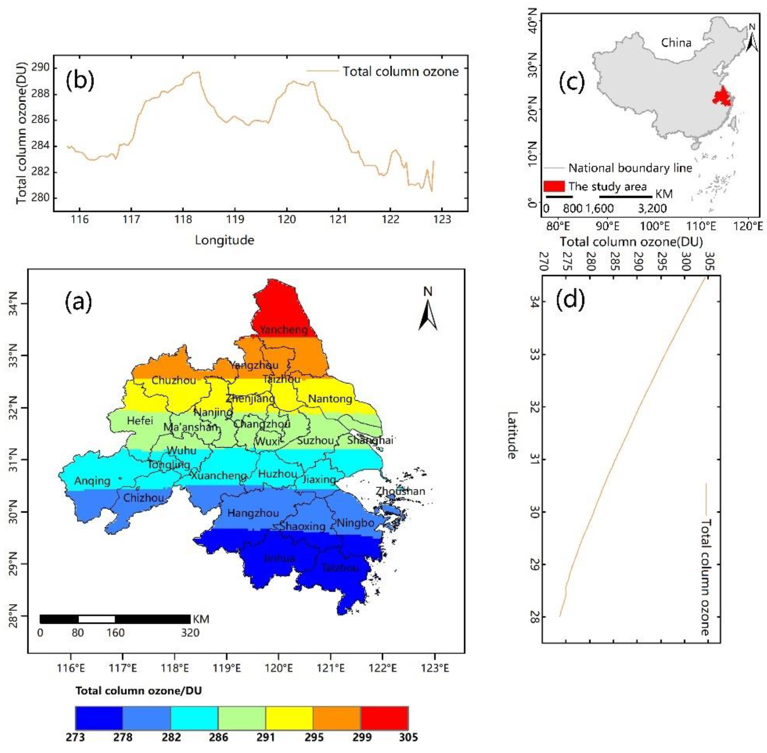
Figure 1. (a) Spatial distribution of the 20-year average TCO over the Yangtze River Delta Urban Agglomerations during 2000–2019. This result was calculated by averaging all annual TCO over the study area. (b) Longitudinal TCO variation in the study area. (c) Location of the study area. (d) Latitudinal TCO variation in the study area.
Remotesensing 14 04576 g001
Figure 2. A line chart of the annual variation in the TCO and the meteorological factors over the Yangtze River Delta Urban Agglomerations during 2000–2019.
Remotesensing 14 04576 g002
Figure 3. The seasonal variation distribution of the TCO over the Yangtze River Delta Urban Agglomerations during 2000–2019. These results were calculated by averaging the monthly data in spring (Spr., the months from March to May in a year) during 2000–2019, and the same progressed for summer (Sum., the months from June to August in a year), autumn (Aut., the months from September to November in a year), and winter (Win., the months from December to February in a year).
Remotesensing 14 04576 g003
Figure 4. The spatial distribution of the 20-year average values of the meteorological factors of temperature (a) precipitation (b) vapor pressure (c) AAI (d) and total solar radiation (e) over the Yangtze River Delta Urban Agglomerations during 2000–2019.
Remotesensing 14 04576 g004
Figure 5. (a) The monthly variation curves of the TCO and meteorological factors over the Yangtze River Delta Urban Agglomerations within a year; (b) the monthly change in the TCO of the Yangtze River Delta Urban Agglomerations during 2000–2019. Note: The TCO and meteorological factors in Figure 5a are the mean values of the same months for all years. Figure 5b shows the monthly variation of the TCO for 20 years.
Remotesensing 14 04576 g005
Figure 6. The fitting line charts of the TCO historical results during 2000–2019 over the Yangtze River Delta Urban Agglomerations by the polynomial function (a), the trigonometric function (b), and the Fourier function (c). Note: The fitted models were constructed based on the annual scale data, so the data corresponding to integer years (such as 2000, 2008, 2009, 2014, etc.) are meaningful and accurate data, and there is little reference in the other values and the fluctuance patterns of the fitting lines; for real interannual changes, please refer to Figure 5b.
Remotesensing 14 04576 g006
Figure 7. The line chart of the TCO prediction results over the Yangtze River Delta Urban Agglomerations during 2020–2030. The red points stand for the TCO prediction results over the study area in each corresponding year. The dotted blue line shows the fitting line of the TCO predicted results based on the constructed Fourier function. The solid gray line is the linear fitting line for the TCO prediction results, and its linear fitting function is shown in the upper-right of the figure. Note: Only the data corresponding to integer years (such as 2020, 2025, 2027, etc.) are meaningful and accurate data, and there is little reference in the other values and the fluctuance patterns of the fitting lines. For more precise interannual changes, please refer to Figure A8.
Remotesensing 14 04576 g007
Table 1. The correlations in the annual variation between the TCO and different meteorological factors.
Air TemperaturePrecipitationVapor PressureAAITotal Solar Radiation
Correlation in Temporal Variation−0.240.380.00−0.01−0.31
Correlation in Spatial Distribution−0.64−0.86−0.590.82−0.60
Note: The absolute value of the correlation coefficients ranging from 0.8 to 1.0 indicate extremely strong correlations; 0.6–0.8 indicates strong correlations; 0.4–0.6 indicates medium-level correlations; 0.2–0.4 indicates weak correlations; 0.0–0.2 indicates extremely weak or no correlations. Correlation in the temporal variation is the time correlations based on the annual values of TCO and meteorological factors during 2000–2019. Correlations in the spatial distribution are the results of spatial autocorrelation analysis by ArcGIS software based on the 20-year average values of the TCO and meteorological factors. The corresponding scatter plot is provided in Figure A4 and Figure A5.
Table 2. The hysteretic response relations between the TCO and different meteorological factors.
Delayed Time (in Months)Air TemperaturePrecipitationVapor PressureAAISolar Radiation
00.170.250.10−0.220.67
1−0.250.01−0.270.110.35
2−0.61−0.25−0.600.41−0.06
3−0.82−0.48−0.790.61−0.48
4−0.79−0.60−0.760.67−0.77
5−0.55−0.53−0.530.54−0.83
6−0.17−0.33−0.150.28−0.67
Table 3. The correlations between the total ozone and economic development of the Yangtze River Delta Urban Agglomerations from 2000 to 2019.
Population SizeRegional GDPRatio of 1st
Industry Value
Ratio of 2nd
Industry Value
Ratio of 3rd
Industry Value
0.937 **0.710 **0.872 **0.897 **0.832 **
Note: The correlations are time correlations and were calculated based on the annual values of the TCO and socioeconomic factors. ** Correlation was significant at the 0.01 level (2-tailed), with significant correlation.
Table 4. The accuracy analysis of the results by different fitting functions.
Fitting FunctionFunction ExpressionNumber of TermsR2SSERMSE
Polynomial Functiony = −1.04833 × 10¹⁵ + 3.13898 × 10¹² × x − 3.9162 × 10⁹ × x2 + 2,605,761.52997 × x3 − 975.26491 × x4 + 0.19467 × x51.61909 × 10−5 × x660.35 **247.7419.06
Trigonometric Functiony = 286.2518 + 7.99065 × sin(pi × (x − 1.24479)/3.14706)-0.26 **281.1317.57
Fourier Functiony = 286.6 − 0.5792 × cos(x × 414) − 0.9698 × sin(x × 414) − 0.5071 × cos(2 × x × 414 − 0.8766 × sin(2 × x × 414) − 1.865 × cos(3 × x × 414) + 2.296 × sin(3 × x × 414) + 2.22 × cos(4 × x × 414) − 1.814 × sin(4 × x × 414) + 0.8274 × cos(5 × x × 414) + 0.2748 × sin(5 × x × 414) − 2.574 × cos(6 × x × 414) − 1.754 × sin(6 × x × 414) − 8.4 × cos(7 × x × 414) + 9.747 × sin(7 × x × 414) + 1.663 × cos(8 × x × 414) − 16.5 × sin(8 × x × 0.414)80.99 **3.361.35
Note: ** Correlation was significant at the 0.01 level (2-tailed) with significant correlation.
Publisher’s Note: MDPI stays neutral with regard to jurisdictional claims in published maps and institutional affiliations.