Article

Pulse Radar Imaging Method in an Anechoic Chamber Based on an Amplitude Modulation Design

State Key Laboratory of Complex Electromagnetic Environmental Effects on Electronics and Information System, National University of Defense Technology, Changsha 410005, China
*
Author to whom correspondence should be addressed.
Remote Sens. 2022, 14(18), 4560; https://doi.org/10.3390/rs14184560
Submission received: 27 June 2022 / Revised: 1 August 2022 / Accepted: 9 September 2022 / Published: 12 September 2022

Abstract

:
The application of a pulse radar in anechoic chamber imaging is a new way to obtain the electromagnetic characteristics of targets. However, the limited size of an anechoic chamber causes the coupling between the transmitted signal and echo so the target image cannot be accurately achieved. To solve this problem, an imaging method using a pulse radar in an anechoic chamber based on an amplitude modulation design is proposed in this paper. Firstly, amplitude modulation is performed to solve the coupling of the transmitted signal and echo. In order to cancel the false targets in the target image after the amplitude modulation, different amplitude modulation sequences are designed. Secondly, echo processing based on the designed amplitude modulation is discussed to obtain the target image. Simulations and experiments are conducted and the results show that the proposed amplitude design and echo processing method can accurately obtain the target image in an anechoic chamber.

1. Introduction

Wideband pulse radar signals are widely used in imaging radars due to their high-range resolution, especially for inverse synthetic aperture radars (ISAR) [1,2,3]. ISAR usually uses the relative motion of the target to image and then obtains the characteristics of the target [4,5]. Currently, field experiments are the main ways to evaluate the imaging performance of the ISAR system and obtain target electromagnetic characteristics. Field experiments are conducted outdoors and are easily affected by non-cooperative interferences so the controllability and reproducibility are poor [6,7,8]. In addition, field experiments require a large experimental space, resulting in difficult management and high costs. Therefore, the experimental data are usually insufficient [9].
In contrast, conducting experiments in an anechoic chamber can overcome the above shortcomings. The process of signal transmission, target reflection, echo reception, and processing can be reproduced in an anechoic chamber so that the radar system can be tested repeatedly and the target electromagnetic characteristics can be obtained at a low cost [10,11]. In addition, the anechoic chamber is an electromagnetic shielding space with high confidentiality. At present, the signals mainly used in anechoic chamber measurements include the impulse pulse and swept frequency signal [12,13,14]. Because the energy of the impulse signal is limited and the equivalent pulse repetition rate of the swept frequency signal is relatively low, the two signals are rarely used in actual radar systems. Instead, pulse radar signals are widely used for target detection and imaging in practical environments. Using pulse radar signals for target imaging in an anechoic chamber can not only obtain the target characteristics but also is not affected by adverse external factors. Thus, it is important to carry out pulse radar imaging experiments in an anechoic chamber.
However, due to the size limitation of an anechoic chamber, the reflected signal is coupled with the transmitted signal so the target cannot be accurately imaged. Inspired by interrupted sampling [15,16,17,18], a pulse radar imaging method based on an amplitude modulation design is proposed in this paper to solve this problem. First, the linear frequency modulation (LFM) signal is divided into many short pulses by designing the amplitude modulation. The duration of each short pulse is less than the arrival time of the echo so that the transmitted signal and the echo are staggered in the time domain to avoid coupling. Then, the imaging method is provided to eliminate the false targets caused by the amplitude modulation. The first segment of echoes within each pulse repetition interval (PRI) is selected and then imaged, and all echoes within each PRI are combined and then imaged. Finally, the real image of the target is obtained by canceling the two images. The novelties and contributions of this paper are summarized as follows.
  • The proposed amplitude modulation method solves the coupling problem between the transmitted signal and echo.
  • The imaging method based on an amplitude modulation design can eliminate the false targets caused by the amplitude-modulated signal and accurately realize the target imaging.
The remainder of this paper is organized as follows. In Section 2, the amplitude modulation design method of the LFM signal is presented. In Section 3, the ISAR imaging method based on an amplitude modulation design and the whole imaging process in an anechoic chamber are given. In Section 4, simulations and experiments are conducted to verify the effectiveness of the proposed method. Finally, conclusions are drawn in Section 5.

2. Amplitude Modulation Design

2.1. Signal Coupling and Amplitude Modulation

The size of an anechoic chamber is usually tens of meters, which is far less than the range corresponding to the pulse width. As shown in Figure 1a, the echo returns before the signal is fully transmitted if the pulse signal is utilized in an anechoic chamber, which causes the coupling in the time domain. The correct target image is difficult to obtain from the mixed transmitted signal and echo. In order to solve the problem, we divide the pulse signal into many short pulses by amplitude modulation, as shown in Figure 1b, ensuring that the transmitted signal and the echo are staggered in the time domain to avoid coupling.
The amplitude modulation function p(t) can be modeled as
p ( t ) = rect ( t / τ ) n = + δ ( t n T s )
where δ(·) is the impulse function, rect(·) is the rectangle function, and “*” represents the convolution operation. p(t) can be viewed as a combination of multiple rectangle functions, τ is the width of a single rectangle function, and Ts is the time interval between two adjacent rectangle functions. The rectangle function can be written as
rect ( t / τ ) = { 1 , | t / τ | < 0.5 0 ,   others
The coupling problem can be solved if the pulse signal is modulated by p(t). The parameter constraints of p(t) are derived in the following equations.
The target size is L and the distance between the target and the antenna is R, the electromagnetic wave velocity is C so the arrival time of the echo is 2R/C. The constraint to ensure that the previous signal is transmitted completely before its echo arrives is
τ 2 R / C
The echo width is τ + 2L/C. The constraint to ensure that the later transmitted signal and the previous echo are staggered in the time domain is
T s τ + 2 L / C + 2 R / C
In summary, the parameter constraints to ensure that the signal after amplitude modulation and its echo are separated in the time domain are
{ τ 2 R / C τ + 2 ( R + L ) / C T s
As long as the parameters τ and Ts satisfy Equation (5), the signal after amplitude modulation and its echo will be staggered in the time domain. As shown in Figure 1b, a pure echo can be obtained by canceling the transmitted signal as it is known previously.

2.2. Properties of Amplitude Modulation Functions

The amplitude modulation function p(t) is shown in Figure 2a. p(t) is shifted downward by λ to obtain the amplitude modulation function pλ(t), as shown in Figure 2b. pλ(t) can be written as
p λ ( t ) = p ( t ) λ = rect ( t / τ ) n = + δ ( t n T s ) λ
where λ is a constant between 0 and 1.
The spectrum of p(t) can be obtained after the Fourier transform
P ( f ) = D n = + sin c ( n D ) δ ( f n f s )
where D = τ/Ts is the duty ratio, fs = 1/Ts, and sinc(x) = sin(πx)/πx. It can be seen in Equation (7) that the spectrum consists of several peaks with a frequency interval of fs, which will cause the spectrum distortion of the pulse signal after amplitude modulation by p(t).
The spectrum of p−λ(t) can be obtained as
P λ ( f ) = D n = + sin c ( n D ) δ ( f n f s ) λ δ ( f )
It can be seen in Equations (7) and (8) that the value of P−λ(f) equals P(f) when n ≠ 0 and f ≠ 0, and the following equation can be obtained:
P ( f ) P λ ( f ) = λ δ ( f )
There are several peaks with a frequency interval of fs in P−λ(f) and P(f). However, only λδ(f) is left after subtracting P−λ(f) from P(f) according to Equation (9). δ(f) is an impulse function and δ(f) ≠ 0 only when f = 0. Thus, all peaks are eliminated, except for λδ(f). This property can be used to recover the spectrum of the pulse signal after amplitude modulation.
Figure 1b shows the schematic diagram of decoupling by amplitude modulation. The complete pulse is divided into many short pulses to ensure that the transmitted signal and the echo are staggered in the time domain to avoid coupling. As a result, the amplitude modulation must be partially 0. Obviously, the amplitude modulation function p(t) meets this requirement, but the amplitude modulation function pλ(t) in Figure 2b should be redesigned. Therefore, the amplitude modulation design is discussed in Section 2.3.

2.3. Amplitude Modulation Design of Pulse Signal

The way to ensure that the p−λ(t) is partially 0 is to decompose it into several parts similar to p(t) as follows.
The amplitude modulation function of the first pulse signal is p1(t) and it can be written as
p 1 ( t ) = ( 1 λ ) rect ( t / τ ) n = + δ ( t n T s )
Let N = ⌈1/D⌉, where ⌈1/D⌉ is the ceil operation of 1/D. The nth pulse signal is modulated by the amplitude modulation function pn(t), n = 2, 3, … , N − 1, and pn(t) can be written as
p n ( t ) = λ ( 1 λ ) p 1 ( t ( n 1 ) τ )
The Nth pulse signal is modulated by the amplitude modulation function pN(t).
p N ( t ) = λ rect [ t ( T s + N τ - 2 τ ) / 2 T s ( N 1 ) τ ] * n = + δ ( t n T s )
The amplitude modulation design of the pulse signal is shown in Figure 3. The first pulse signal is modulated by p1(t) to obtain the first transmission signal (red waveform) and the second pulse signal is modulated by p2(t) to obtain the second transmission signal (yellow waveform), and so on. The Nth pulse signal is modulated by pN(t) to obtain the Nth transmission signal (green waveform). After the target scattering, the first segment of the echo is selected and multiplied by 1/(1 − λ) according to Equations (1) and (10), which is called amplitude compensation. Then the echo modulated by p(t) is equivalently obtained. At the same time, all amplitude-modulated echoes are combined according to their relative positions in Figure 2b, which is called echo combination. Then, the echo modulated by pλ(t) is equivalently obtained.

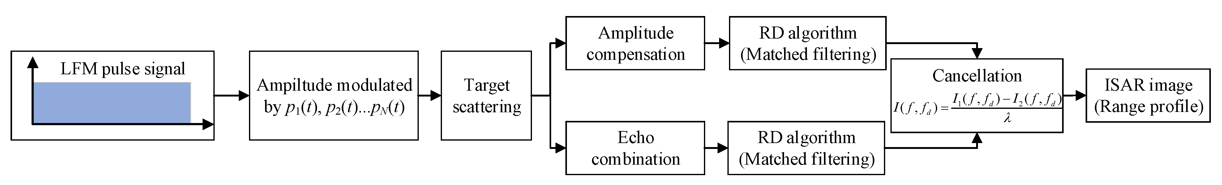
3. Target Imaging Method

3.1. Range Profile Acquisition Based on Amplitude Modulation Design

The transmitting signal is the LFM signal and the echo is
S ( t ) = k = 1 K X k ( t )
where the target has K scattering points, Xk(t) is the echo of the kth scattering point, and its expression is
X k ( t ) = α k rect [ t 2 R k / C T p ] exp { j π [ 2 f 0 ( t 2 R k C ) + μ ( t 2 R k C ) 2 ] }
where αk is the scattering coefficient of the kth scattering point, f0 is the carrier frequency, Tp is the single pulse width, B is the bandwidth, μ = B/Tp is the chirp rate, and Rk is the distance between the kth scattering point and the antenna.
The dechirp reference signal is
S r e f ( t ) = rect ( t T r e f ) exp [ j 2 π ( f 0 t + 0.5 μ t 2 ) ]
where Tref is the duration of the reference dechirp signal.
According to the dechirp principle, the difference-frequency output is
S y ( t ) = S ( t ) S r e f * ( t )
where Sref*(t) is the conjugation of Sref(t).
Denote the range profile of the LFM signal as y(f) and it can be obtained after the Fourier transform of Sy(t)
y ( f ) = T p k = 1 K α k sin c [ T p ( f + 2 μ C R k ) ] exp ( j 4 π f 0 C R k )
The echo of the LFM signal modulated by p(t) is
S 1 ( t ) = k = 1 K p ( t 2 R k C ) X k ( t )
The difference-frequency output of S1(t) is
S y 1 ( t ) = S 1 ( t ) S r e f * ( t )
Denote the range profile of the LFM signal modulated by p(t) as y1(f) and it can be obtained after the Fourier transform of Sy1(t)
y 1 ( f ) = τ f s T p k = 1 K { α k exp ( j 4 π f 0 C R k ) n = n = + sin c ( n f s τ ) sin c [ T p ( f n f s + 2 μ C R k ) ] }
Compared with Equation (17), there are many false peaks in the range profile of the LFM signal modulated by p(t). From Equation (20), we can see that y1(f) is the sum of the range profiles of K scattering points. For the kth scattering point, the main part of y1(f) is the product of two sinc functions. The property of sinc(x) is that its peak occurs at x = 0. We only focus on the second sinc function as sinc(nfsτ) is independent of f. Obviously, its peak appears at nfs − (2μRk)/C and (2μRk)/C is a constant for the kth scattering point. Thus, the interval of the adjacent peaks in the frequency domain is fs and the interval in the distance is Cfs/(2μ) according to the characteristics of the LFM signal.
The echo of the LFM signal modulated by pλ(t) is
S 2 ( t ) = k = 1 K [ p ( t 2 R k C ) λ ] X k ( t )
The difference-frequency output of S2(t) is
S y 2 ( t ) = S 2 ( t ) S r e f * ( t )
Denote the range profile of the LFM signal modulated by p−λ(t) as y2(f) and it can be obtained after the Fourier transform of Sy2(t)
y 2 ( f ) = τ f s T p k = 1 K { α k exp ( j 4 π f 0 C R k ) n = n = + sin c ( n f s τ ) sin c [ T p ( f n f s + 2 μ C R k ) ] } λ T p k = 1 K α k sin c [ T p ( f + 2 μ C R k ) ] exp ( j 4 π f 0 C R k )
Similar to the analysis of Equation (20), it can be seen in Equation (23) that there are also false peaks in y2(f). The interval of the adjacent peaks in the frequency domain is fs and the interval in the distance is Cfs/(). However, according to Equations (17), (20), and (23), the following equation can be obtained:
y ( f ) = [ y 1 ( f ) y 2 ( f ) ] λ
According to Equation (24), y(f) can be obtained by subtracting y2(f) from y1(f) and then multiplying by 1/λ, which is called cancellation. The false peaks caused by amplitude modulation can be eliminated by cancellation, and the range profile after cancellation is the same as the range profile of the LFM signal. Thus, if we use the two amplitude modulation functions in Figure 2 to modulate the LFM signal in an anechoic chamber, the target range profile can be obtained according to Equation (24).

3.2. ISAR Imaging Based on Amplitude Modulation Design

From Section 3.1, we know that the range profile will appear with false peaks after LFM signals are modulated by p(t) and pλ(t). After imaging with the Range Doppler (RD) algorithm, false targets will also appear in the range dimension of the ISAR image. Thus, based on the range profile properties after amplitude modulation, the false image cancellation method is discussed to obtain the correct target image.
Considering an ideal scene where the isolation is so high that the coupling can be ignored, the results of ISAR imaging with theLFM signal are derived as follows. After the translational motion compensation, the target can be regarded as a turnable model rotating around its origin [19,20] and the turntable model is the basis for the derivation in this section.
The LFM signal echo at a certain slow time tm is S(t, tm).
S ( t , t m ) = k = 1 K X k ( t , t m )
where the target has K scattering points, Xk(t, tm) is the LFM signal echo of the kth scattering point at a certain slow time tm, and its expression is
X k ( t , t m ) = α k rect [ t 2 R k ( t m ) / C T p ] exp { j π [ 2 f 0 ( t 2 R k ( t m ) C ) + μ ( t 2 R k ( t m ) C ) 2 ] }
where αk is the scattering coefficient of the kth scattering point, t is the fast time, Rk(tm) is the distance between the kth scattering point and the antenna at a certain slow time tm, and Rk(tm) is a variable about tm as the target rotates around its origin.
The dechirp reference signal at each slow time tm is
S r e f ( t , t m ) = r e c t ( t T r e f ) exp [ j 2 π ( f 0 t + 0.5 u t 2 ) ]
Denote the ISAR imaging result of the LFM signal as I(f, fd). According to the RD algorithm, I(f, fd) can be written as
I ( f , f d ) = k = 1 K FFT t m [ FFT t ( X k ( t , t m ) S r e f * ( t , t m ) ) ]
where S*ref(t, tm) is the conjugate operation of Sref(t, tm), FFTt is the fast Fourier transform of the fast time t, and FFTtm is the fast Fourier transform of the slow time tm.
The echo of the LFM signal modulated by p(t) is S1(t, tm), and S1(t, tm) can be written as
S 1 ( t , t m ) = k = 1 K p ( t 2 R k ( t m ) C ) X k ( t , t m )
where 2Rk(tm)/C is the time delay caused by the kth scattering point. Xk(t, tm) is the echo of the LFM signal. p(t − 2Rk(tm)/C) is the amplitude modulation function considering the time delay. p(t − 2Rk(tm)/C)Xk(t, tm) is the echo of the kth scattering point of the LFM signal modulated by p(t) and S1(t, tm) is the sum of the echoes of K scattering points.
Denote the ISAR imaging result of S1(t, tm) as I1(f, fd). According to the RD algorithm, I1(f, fd) can be written as
I 1 ( f , f d ) = = k = 1 K FFT t m { FFT t [ p ( t 2 R k ( t m ) C ) ] * FFT t ( X k ( t , t m ) S r e f * ( t , t m ) ) }
The echo of the LFM signal modulated by pλ(t) is S2(t, tm), and S2(t, tm) can be written as
S 2 ( t , t m ) = k = 1 K [ p ( t 2 R k ( t m ) C ) λ ] X k ( t , t m )
where 2Rk(tm)/C is the time delay caused by the kth scattering point. Xk(t, tm) is the echo of the LFM signal. p(t − 2Rk(tm)/C) – λ is the amplitude modulation function considering the time delay. [p(t − 2Rk(tm)/C) – λ]Xk(t, tm) is the echo of the kth scattering point of the LFM signal modulated by p(t) and S2(t, tm) is the sum of the echoes of K scattering points.
Denote the ISAR imaging result of S2(t, tm) as I2(f, fd). According to the RD algorithm, I2(f, fd) can be written as
I 2 ( f , f d ) = k = 1 K FFT t m { FFT t [ p ( t 2 R k ( t m ) C ) ] * FFT t ( X k ( t , t m ) S r e f * ( t , t m ) ) } λ k = 1 K FFT t m { FFT t ( X k ( t , t m ) S r e f * ( t , t m ) ) }
According to Equations (28), (30), and (32), the following equation can be obtained
I ( f , f d ) = I 1 ( f , f d ) I 2 ( f , f d ) λ
The false targets caused by amplitude modulation can be eliminated according to Equation (33). The echoes of the LFM signals modulated by p(t) and pλ(t) can be obtained as in Figure 3. Their echoes are imaged and then the real target image is obtained by image cancellation according to Equation (33).

3.3. Imaging Process in Anechoic Chamber

The imaging process based on an amplitude modulation design is shown in Figure 4. The specific steps are as follows.
Step 1: The LFM signal is transmitted after amplitude modulation by p1(t), p2(t),…, pN(t).
Step 2: The specific methods of amplitude compensation and echo combination are defined in Section 2.3. After target scattering, the echo modulated by p(t) is equivalently obtained by amplitude compensation of the first segment of the echo. The echo modulated by p-λ(t) is equivalently obtained by echo combination.
Step 3: The echoes modulated by p(t) and pλ(t) are imaged by the RD algorithm, respectively, and then canceled to obtain the real target image according to Equation (33). When acquiring the target range profile, the difference is that matched filtering is required after amplitude compensation and echo combination, instead of using the RD algorithm.

4. Simulation and Experiment

In order to verify the effectiveness of the proposed method, numerical simulations are first carried out in Section 4.1. Then, the influence of the signal-to-noise ratio (SNR) on the correlation coefficient is analyzed in Section 4.2. Finally, anechoic chamber experiments are carried out in Section 4.3.

4.1. Numerical Simulation

4.1.1. Range Profile Simulation

In this section, numerical simulations of the range profile are carried out. The simulation parameters of the range profile are listed in Table 1. According to Equation (5), set Ts = 0.9 μs, τ = 0.36 μs. The imaging process is shown in Figure 4 and the range profile simulation results are shown in Figure 5.
The duty ratio D is 0.4 so the amplitude modulation functions p1(t), p2(t), and p3(t) are used to modulate the LFM signal and the echo is shown in Figure 5a. The echo modulated by p(t) is obtained by amplitude compensation of the first segment of the echo then, its range profile is obtained by dechirp processing and the range profile is shown in Figure 5b. The echo modulated by p−λ(t) is obtained by echo combination then, its range profile is obtained by dechirp processing, as shown in Figure 5c. It can be seen in Figure 5b,c that there are false peaks in the range profile of the LFM signals after amplitude modulation. However, the real target range profile can be obtained by cancellation with Figure 5b,c. Figure 5d presents the comparison of the range profile after cancellation and the complete LFM range profile. It is worth noting that the range profile of the LFM signal is an ideal result based on the assumption that the isolation between antennas is high enough to ignore the coupling, and it is a reference used to evaluate the imaging effect of the method proposed in this paper. As shown in Figure 5d, the range profile after cancellation coincides with the range profile of the LFM signal, and the characteristics of the range profile, such as the range resolution, remain unchanged.

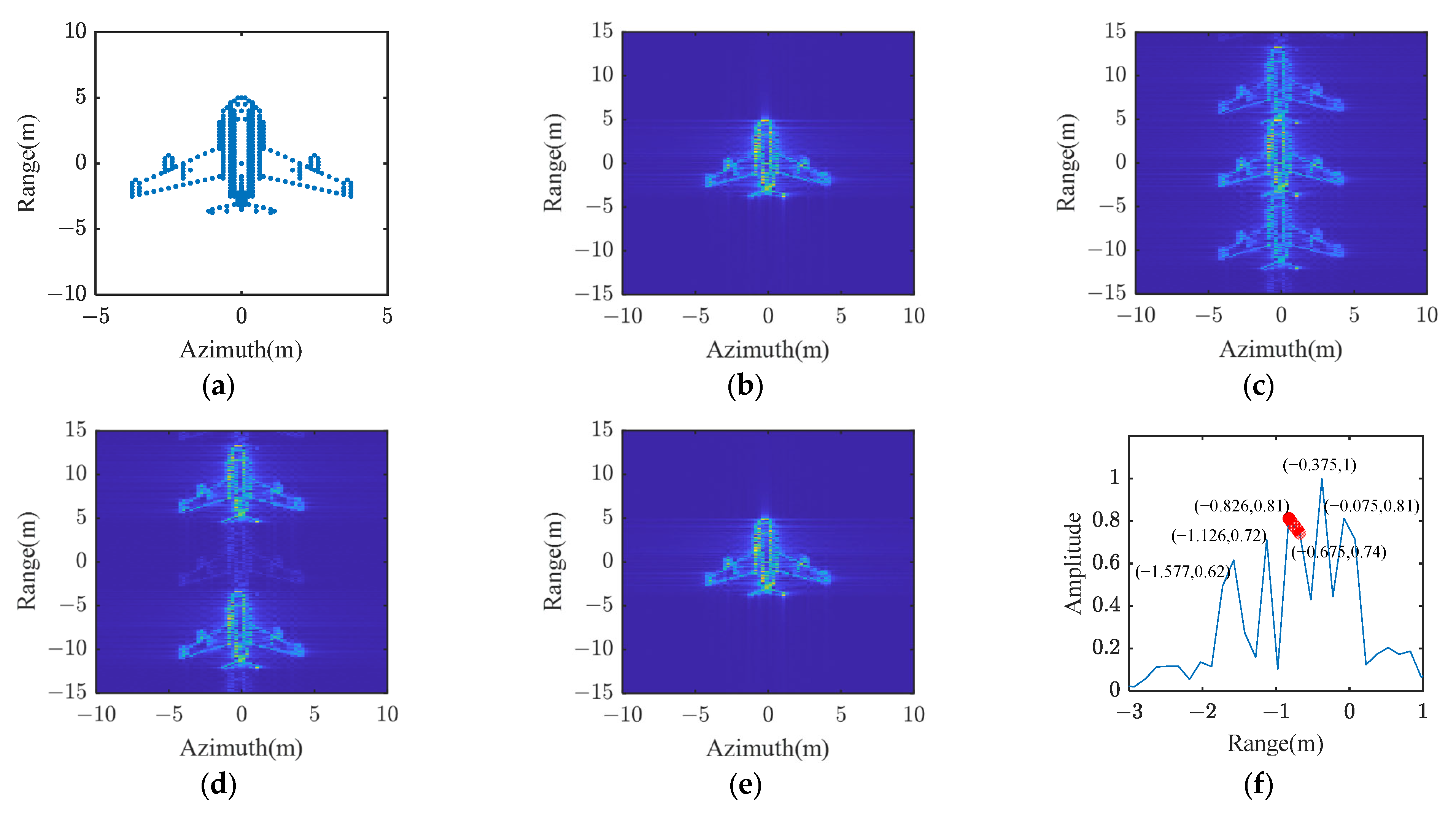
4.1.2. ISAR Imaging Simulation

Consider the following ISAR imaging simulation scenarios. The target is a Yak-42 aircraft model with 330 scattering points. The distance between the target and antennas is 80 m and the target rotation angular velocity is 0.05π rad/s. The signal parameters are the same as in Table 1. The PRI is 1 ms and the imaging accumulation time is 400 ms. The imaging process is revealed in Figure 4, and the imaging results of the Yak-42 aircraft model based on an amplitude modulation design are shown in Figure 6.
Figure 6a is the 330 scattering-points model of the Yak-42 aircraft. The size is 8.75 m (range direction) × 7.5 m (azimuth direction). Assuming that the isolation between antennas is high enough to ignore the coupling, we obtain the ideal ISAR imaging result of the complete LFM signal, as shown in Figure 6b. The duty ratio of the amplitude modulation function is D = 0.4. According to Section 2.3, the number of LFM signals continuously transmitted in each PRI is N = ⌈1/D⌉ = 3. After the target scattering, the first segment of the echo in each PRI is selected for amplitude compensation so the echo modulated by p(t) is equivalently obtained. Then the RD algorithm is used to obtain the image in Figure 6c. The echoes of each PRI are combined to obtain the echoes modulated by pλ(t) equivalently, and then the RD algorithm is used to obtain the image in Figure 6d. It can be seen in Figure 6c,d that there are false targets in the ISAR images of the LFM signals after amplitude modulating by p(t) and pλ(t). According to Equation (33), Figure 6c,d are canceled to obtain the real image of the Yak-42 aircraft model in Figure 6e. The size of the Yak-42 aircraft model and the locations of the scattering points are basically the same as in Figure 6b.
Figure 6a is the 330 scattering-points model of the Yak-42 aircraft. The size is 8.75 m (range direction) × 7.5 m (azimuth direction). Assuming that the isolation between antennas is high enough to ignore the coupling, we obtain the ideal ISAR imaging result of the complete LFM signal, as shown in b. The duty ratio of the amplitude modulation function is D = 0.4. According to Section 2.3, the number of LFM signals continuously transmitted in each PRI is N = ⌈1/D⌉ = 3. After the target scattering, the first segment of the echo in each PRI is selected for amplitude compensation so the echo modulated by p(t) is equivalently obtained. Then the RD algorithm is used to obtain the image in c. The echoes of each PRI are combined to obtain the echoes modulated by pλ(t) equivalently, and then the RD algorithm is used to obtain the image in Figure 6d. It can be seen in Figure 6c,d that there are false targets in the ISAR images of the LFM signals after amplitude modulating by p(t) and pλ(t). According to Equation (33), Figure 6c,d are canceled to obtain the real image of the Yak-42 aircraft model in Figure 6e. The size of the Yak-42 aircraft model and the locations of the scattering points are basically the same as in Figure 6b.
The range profile with an azimuth of −2 m is shown in Figure 6f. It can be seen in Figure 6f that when the azimuth is −2 m, there are five scattering points and their positions are [−1.577 m, −1.126 m, −0.826 m, −0.675 m, −0.375 m, −0.075 m]. When the azimuth is −2 m, the aircraft model in Figure 6a has 5 scattering points and the positions are [−1.625 m, −1.125 m, −0.865 m, −0.625 m, −0.375 m, −0.125 m]. The relative error of each scattering point is less than 5%, which proves that the imaging method based on an amplitude modulation design proposed in this paper is effective and can accurately obtain the characteristics of the target.

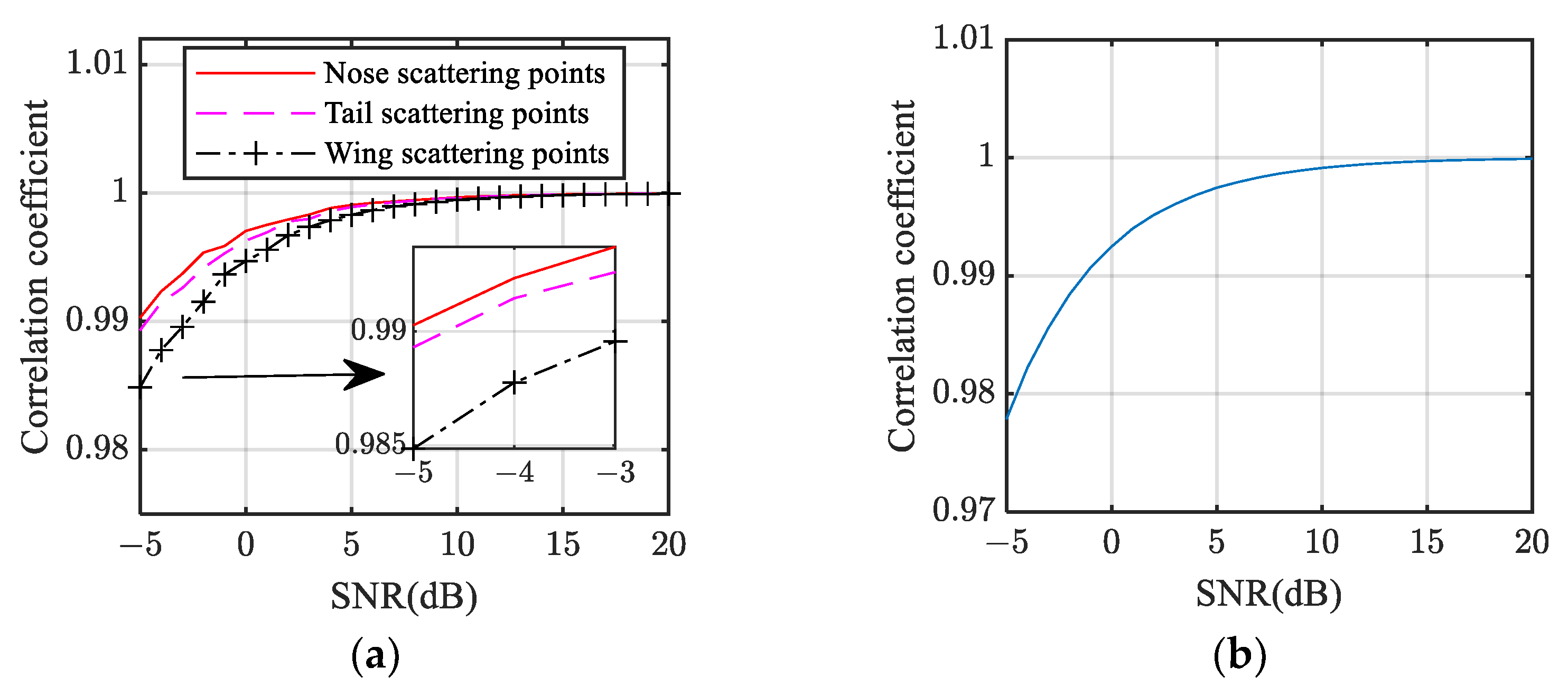
4.2. Influence of SNR on Correlation Coefficient

Although the original LFM signal cannot be used for imaging in an anechoic chamber, we can obtain the theoretical imaging result of the original LFM signal by assuming that the isolation between antennas is high enough to ignore the coupling. Then, the correlation coefficients between the imaging results of the original LFM signal and the imaging results based on the proposed method are calculated to evaluate the effectiveness of the proposed method. According to [21,22], the correlation coefficient between the two N × M blocks of images IA and IB is defined as
C o r r ( I A , I B ) = m = 1 M n = 1 N ( I A ( m , n ) a 0 ) ( I B ( m , n ) b 0 ) m = 1 M n = 1 N ( I A ( m , n ) a 0 ) 2 m = 1 M n = 1 N ( I B ( m , n ) b 0 ) 2
where IA(m, n) is the intensity of the (m, n)th pixel in image IA, IB(m, n) is the intensity of the (m, n)th pixel in image IB, and a0 and b0 are the mean intensity values of image IA and IB, respectively. The correlation coefficients are calculated under different SNRs and the results are shown in Figure 7.
The correlation coefficients of the aircraft nose, tail, and wing are calculated, respectively, and the results are shown in Figure 7a. When the SNR is the same, the correlation coefficient of the nose is the largest, followed by the tail, and the wing is the smallest. It is because the average scattering coefficients of the aircraft nose, tail, and wing are [0.75, 0.5, 0.35]. The imaging performance is positively correlated with the scattering coefficient. When the SNR is −5 dB, the correlation coefficients of the aircraft nose, tail, and wing are higher than 0.985. In addition, their correlation coefficients increase as the SNR increases. Figure 7b presents the correlation coefficient of the whole image. The variation trend of the correlation coefficient in Figure 7b is similar to that in Figure 7a. The nose, wing, and tail are strong scattering points in the aircraft so the correlation coefficients are higher than the correlation coefficient of the whole image. In general, the correlation coefficients are at a high level, which verifies the effectiveness of the imaging method proposed in this paper.

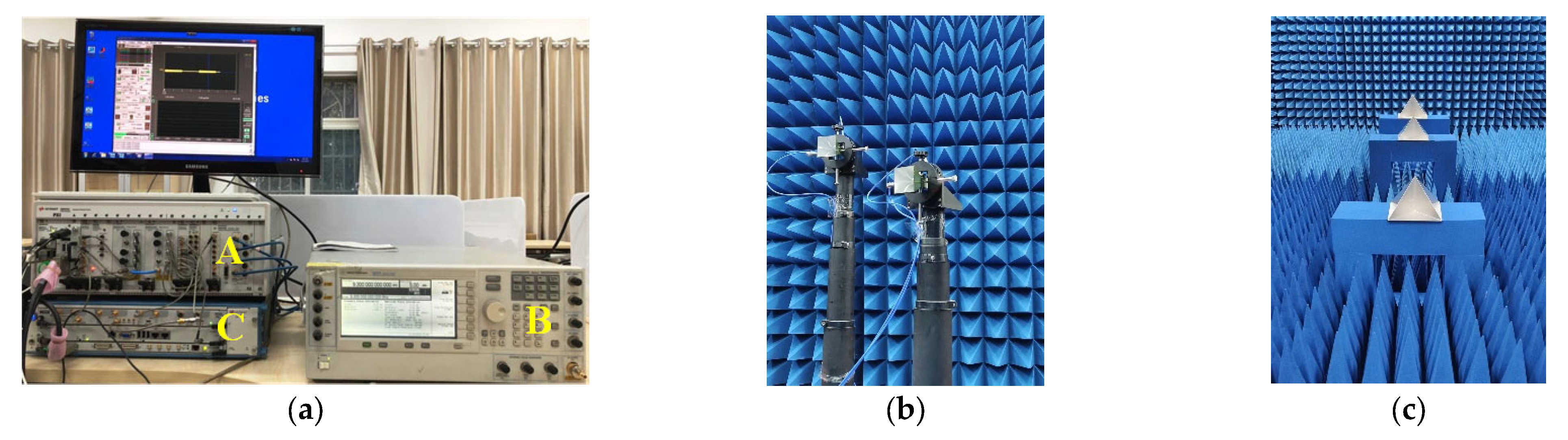
4.3. Anechoic Chamber Experimental Results

On the basis of the numerical simulation, the effectiveness of the imaging method based on an amplitude modulation design is further verified by anechoic chamber experiments. The range profile experiment and the unmanned aerial vehicle (UAV) ISAR imaging experiment are carried out in this section.

4.3.1. Experiment Results of Range Profile

Figure 8a is the experimental system that contains three parts. Part A is the arbitrary waveform generator (AWG). The LFM signal with 500 MHz and 12 μs is generated by the AWG. Part B is the up-converter to up-convert the baseband signal to 9 GHz. Part C is the data acquisition to store the target echo. Figure 8b shows the transmit and receive antennas. Figure 8c shows the three reflectors used to simulate the target scattering centers. The distance between the reflectors and the antennas is [21 m, 23.2 m, 24.9 m]. The results of the range profile experiment are presented in Figure 9.
The echo of the LFM signal after amplitude modulation is shown in Figure 9a. The range profile of the first segment of the echo and the combined echo are shown in Figure 9b,c. There are false peaks in Figure 9b,c. However, after cancellation, the real target range profile can be obtained, as shown in Figure 9d. It can be seen in Figure 9d that there are three peaks and the position of the peaks are correct.

4.3.2. Experiment Results of ISAR Imaging

To further verify the imaging performance of the proposed method, the unmanned aerial vehicle (UAV)-measured data in an anechoic chamber is used in Section 4.3.2.
The pioneer UAV model is shown in Figure 10a. The measurement scene of the UAV in an anechoic chamber is shown in Figure 10b and the Pioneer UAV model rotates under the control of the turntable. The UAV is 2.3 m long with a wingspan of 2.9 m and a height of 0.66 m. The nose direction is placed along the X-axis and is defined as 0° in the azimuth direction.
The signal parameters are shown in Table 2. The transmitted signal consists of 200 sub-pulses with a frequency range from 8 GHz to 12 GHz and a bandwidth of 4 GHz. The parameters of the amplitude modulation functions are Ts = 0.9 μs, τ = 0.36 μs. The UAV imaging results in the anechoic chamber based on an amplitude modulation design are shown in Figure 11.
The imaging result of the first segment of the echo is presented in Figure 11a. The imaging result of the combined echo is presented in Figure 11b. There are false targets in Figure 11a,b. However, after cancellation by Figure 11a,b, the real image of the UAV is obtained in Figure 11c. The ISAR image in Figure 11c accurately obtains the size, shape, and other information of the UAV, which verifies the effectiveness of the proposed method.

5. Conclusions

An amplitude modulation design is proposed in this paper to solve the problem where the pulse signal cannot be used for anechoic chamber imaging because of coupling. Based on the analysis of the properties of the amplitude modulation functions, the amplitude modulation design method of the LFM signal is given. Furthermore, the properties of the LFM signal after amplitude modulation are analyzed and then the corresponding imaging method is provided. The numerical simulation and experiment results illustrate that the corresponding imaging method can effectively eliminate the false targets caused by the LFM signal after amplitude modulation and realize the target imaging. Amplitude modulation design is of significance for pulse radar target imaging and recognition in anechoic chambers in the future.

Author Contributions

Conceptualization, S.X. and F.Z.; methodology, X.L. and F.Z.; software, X.L. and A.X.; validation, A.X.; formal analysis, A.X. and X.L.; data curation, A.X.; writing—original draft preparation, A.X. and X.L.; writing—review and editing, A.X., F.Z. and X.L.; visualization, A.X. and X.L.; funding acquisition, F.Z. All authors have read and agreed to the published version of the manuscript.

Funding

This work was supported in part by the National Natural Science Foundation of China under Grant 61890542 and Grant 62001481, and in part by the Natural Science Foundation of Hunan Province under Grant 2020JJ40686.

Data Availability Statement

Not applicable.

Conflicts of Interest

The authors declare no conflict of interest.

References

  1. Liu, F.; Huang, D.; Guo, X.; Feng, C. Unambiguous ISAR Imaging Method for Complex Maneuvering Group Targets. Remote Sens. 2022, 14, 2554. [Google Scholar] [CrossRef]
  2. Wei, S.; Zhang, L.; Liu, H. Integrated Kalman filter of accurate ranging and tracking with wideband radar. IEEE Trans. Geosci. Remote Sens. 2022, 58, 8395–8411. [Google Scholar] [CrossRef]
  3. Yang, S.; Li, S.; Jia, X.; Liu, Y. An Efficient Translational Motion Compensation Approach for ISAR Imaging of Rapidly Spinning Targets. Remote Sens. 2022, 14, 2208. [Google Scholar] [CrossRef]
  4. Li, H.; Liao, G.; Xu, J.; Lan, L. An Efficient Maritime Target Joint Detection and Imaging Method with Airborne ISAR System. Remote Sens. 2022, 14, 193. [Google Scholar] [CrossRef]
  5. Yang, Z.; Li, D.; Tan, X.; Liu, H.; Liu, Y.; Liao, G. ISAR Imaging for Maneuvering Targets with Complex Motion Based on Generalized Radon-Fourier Transform and Gradient-Based Descent under Low SNR. Remote Sens. 2021, 13, 2198. [Google Scholar] [CrossRef]
  6. Fan, W.; Kyösti, P.; Hentilä, L.; Pedersen, G.F. Experimental Evaluation of MIMO Terminals with User Influence in OTA Setups. IEEE Antennas Wirel. Propag. Lett. 2017, 16, 3030–3033. [Google Scholar] [CrossRef]
  7. Hashim, M.; Stavrou, S. Dynamic impact characterization of vegetation movements on radiowave propagation in controlled environment. IEEE Antennas Wirel. Propag. Lett. 2003, 2, 316–318. [Google Scholar] [CrossRef]
  8. Tice, T.E. An overview of radar cross section measurement techniques. In Proceedings of the Instrumentation and Measurement Technology Conference, Washington, DC, USA, 25–27 April 1989; pp. 344–346. [Google Scholar]
  9. Liu, X.; Liu, J.; Zhao, F.; Ai, X.; Wang, G. A novel strategy for pulse radar HRRP reconstruction based on randomly interrupted transmitting and receiving in radio frequency simulation. IEEE Trans. Antennas Propag. 2018, 66, 2569–2580. [Google Scholar] [CrossRef]
  10. Huang, H.; Pan, M.; Lu, Z. Hardware-in-the-loop simulation technology of wide-band radar targets based on scattering center model. Chin. J. Aeronaut. 2015, 28, 1476–1484. [Google Scholar] [CrossRef]
  11. Lee, J.; Kim, H.; Myung, N. Analysis of structural anechoic chamber design for improvement of anechoic chamber performance. In Proceedings of the 2015 Asia-Pacific Microwave Conference (APMC), Nanjing, China, 6–9 December 2015; pp. 1–3. [Google Scholar]
  12. Chen, X.; Kildal, P.; Carlsson, J.; Yang, J. MRC diversity and MIMO capacity evaluations of multi-port antennas using reverberation chamber and anechoic chamber. IEEE Trans. Antennas Propag. 2013, 61, 917–926. [Google Scholar] [CrossRef] [Green Version]
  13. He, L.; Xue, Z.; Ren, W.; Li, W. S-band time domain near field planar measurement for RCS inside an anechoic chamber. In Proceedings of the 2015 7th Asia-Pacific Conference on Environmental Electromagnetics (CEEM), Hangzhou, China, 4 January 2016; pp. 108–111. [Google Scholar]
  14. Kudyan, H.M. Sensitivity of frequency-swept shielding effectiveness measurements to reflecting surfaces and EMI noise in the test area. In Proceedings of the 2003 IEEE Symposium on Electromagnetic Compatibility, Boston, MA, USA, 14 October 2003; pp. 526–531. [Google Scholar]
  15. Lu, L.; Gao, M. A Truncated Matched Filter Method for Interrupted Sampling Repeater Jamming Suppression Based on Jamming Reconstruction. Remote Sens. 2022, 14, 97. [Google Scholar] [CrossRef]
  16. Wang, F.; Li, N.; Pang, C.; Li, C.; Li, Y.; Wang, X. Complementary Sequences and Receiving Filters Design for Suppressing Interrupted Sampling Repeater Jamming. IEEE Geosci. Remote Sens. Lett. 2022, 19, 1–5. [Google Scholar]
  17. Wu, W.; Zou, J.; Chen, J.; Xu, S.; Chen, Z. False-target recognition against interrupted-sampling repeater jamming based on integration decomposition. IEEE Trans. Aerosp. Electron. Syst. 2021, 57, 2979–2991. [Google Scholar] [CrossRef]
  18. Zhou, C.; Liu, Q.; Chen, X. Parameter estimation and suppression for DRFM-based interrupted sampling repeater jammer. IET Radar Sonar Navig. 2018, 12, 56–63. [Google Scholar] [CrossRef]
  19. Tan, X.; Yang, Z.; Li, D.; Liu, H.; Liao, G.; Wu, Y.; Liu, Y. An efficient range-Doppler domain ISAR imaging approach for rapidly spinning targets. IEEE Trans. Geosci. Remote Sen. 2019, 58, 2670–2681. [Google Scholar] [CrossRef]
  20. Qian, J.; Huang, S.; Wang, L.; Bi, G.; Yang, X. Super-resolution ISAR imaging for maneuvering target based on deep-learning-assisted time–frequency analysis. IEEE Trans. Geosci. Remote Sens. 2021, 60, 1–14. [Google Scholar] [CrossRef]
  21. Gupta, N.; Bhargava, N.; Verma, B.; Khan, M.I.; Kumar, S. A New Approach for CBIR Using Coefficient of Correlation. In Proceedings of the 2009 International Conference on Advances in Computing, Control, and Telecommunication Technologies, Bangalore, India, 28–29 December 2009; pp. 380–384. [Google Scholar]
  22. Naji, M.A.; Aghagolzadeh, A. Multi-focus image fusion in DCT domain based on correlation coefficient. In Proceedings of the 2015 2nd International Conference on Knowledge-Based Engineering and Innovation (KBEI), Tehran, Iran, 21 March 2016; pp. 632–639. [Google Scholar]
Figure 1. Signal coupling and decoupling by amplitude modulation: (a) Coupling diagram; (b) Decoupling by amplitude modulation.
Remotesensing 14 04560 g001
Figure 2. Amplitude modulation function: (a) Amplitude modulation function p(t); (b) Amplitude modulation function p−λ(t).
Remotesensing 14 04560 g002
Figure 3. Amplitude modulation design of pulse signal.
Remotesensing 14 04560 g003
Figure 4. Imaging process based on amplitude modulation design.
Remotesensing 14 04560 g004
Figure 5. Range profile simulation results: (a) LFM signal echo after amplitude modulation; (b) Range profile of the first segment of the echo; (c) Range profile of the combined echo; (d) Range profile comparison.
Remotesensing 14 04560 g005
Figure 6. Imaging results of Yak-42 aircraft model: (a) Yak-42 aircraft model; (b) Imaging result of the complete LFM signal; (c) Imaging result of the first segment of the echo; (d) Imaging result of the combined echo; (e) Imaging result after cancellation; (f) Range profile with an azimuth of −2 m.
Remotesensing 14 04560 g006
Figure 7. Correlation coefficients at different SNRs: (a) Correlation coefficients of specific scattering points; (b) Correlation coefficient of the whole image.
Remotesensing 14 04560 g007
Figure 8. Figure 8. Measurement scene in the anechoic chamber: (a) Experiment system; (b) Antennas; (c) Targets.
Remotesensing 14 04560 g008
Figure 9. Measurement results: (a) Echo in the anechoic chamber; (b) Range profile of the first segment of echo; (c) Range profile of the combined echo; (d) Range profile after cancellation.
Remotesensing 14 04560 g009
Figure 10. UAV model and measurement scene in the anechoic chamber: (a) Pioneer UAV model; (b) Measurement scene in the anechoic chamber.
Remotesensing 14 04560 g010
Figure 11. UAV imaging results in an anechoic chamber: (a) Imaging result of the first segment of the echo; (b) Imaging result of the combined echo; (c) Imaging result after cancellation.
Remotesensing 14 04560 g011
Table 1. Parameters of range profile simulation.
ParameterValue
Pulse width50 μs
Bandwidth1 GHz
Wavelength0.0375 m
Distances of scattering centers[0 m, 1 m, 4.1 m]
Scattering coefficients[0.7, 0.5, 0.9]
Duty ratio D0.4
Table 2. Signal parameters.
ParameterValue
Initial frequency8 GHz
Terminal frequency12 GHz
Bandwidth4 GHz
Number of sub-pulses200
Pitch angle
Azimuth angle−180~180°
Azimuth interval0.2°
Publisher’s Note: MDPI stays neutral with regard to jurisdictional claims in published maps and institutional affiliations.

