Article

Application and Analysis of XCO2 Data from OCO Satellite Using a Synthetic DINEOF–BME Spatiotemporal Interpolation Framework

1
Ocean College, Zhejiang University, Zhoushan 316000, China
2
Ocean Academy, Zhejiang University, Zhoushan 316000, China
3
Department of Geography, San Diego State University, San Diego, CA 92108, USA
*
Author to whom correspondence should be addressed.
Remote Sens. 2022, 14(17), 4422; https://doi.org/10.3390/rs14174422
Submission received: 14 July 2022 / Revised: 17 August 2022 / Accepted: 21 August 2022 / Published: 5 September 2022

Abstract

:
Carbon dioxide (CO2) is one of the main greenhouse gases leading to global warming, and the ocean is the largest carbon reservoir on the earth that plays an important role in regulating CO2 concentration on a global scale. The column-averaged dry-air mole fraction of atmospheric CO2 (XCO2) is a key parameter in describing ocean carbon content. In this paper, the Data Interpolation Empirical Orthogonal Function (DINEOF) and the Bayesian Maximum Entropy (BME) methods are combined to interpolate XCO2 data of Orbiting Carbon Observatory 2 (OCO-2) and Orbiting Carbon Observatory 3 (OCO-3) from January to December 2020 occurring within the geographical range of 15–45°N and 120–150°E. At the first stage of our proposed analysis, spatiotemporal information was used by the DINEOF method to perform XCO2 interpolation that improved data coverage; at the second stage, the DINEOF-generated interpolation results were regarded as soft data and were subsequently assimilated using the BME method to obtain improved XCO2 interpolation values. The performance of the synthetic DINEOF–BME interpolation method was evaluated by means of a five-fold cross-validation method. The results showed that the Mean Absolute Error (MAE), the Root Mean Square Error (RMSE), and the Bias of the DINEOF-based OCO-2 and OCO-3 interpolations were 2.106 ppm, 3.046 ppm, and 1.035 ppm, respectively. On the other hand, the MAE, RMSE, and Bias of the cross-validation results obtained by the DINEOF–BME were 1.285 ppm, 2.422 ppm, and −0.085 ppm, respectively, i.e., smaller than the results obtained by DINEOF. In addition, based on the in situ measured XCO2 data provided by the Total Carbon Column Observing Network (TCCON), the original OCO-2 and OCO-3 data were combined and compared with the interpolated products of the synthetic DINEOF–BME framework. The accuracy of the original OCO-2 and OCO-3 products is lower than the DINEOF–BME-generated XCO2 products in terms of MAE (1.751 ppm vs. 2.616 ppm), RMSE (2.877 ppm vs. 3.566 ppm) and Bias (1.379 ppm vs 1.622 ppm), the spatiotemporal coverage of XCO2 product also improved dramatically from 16% to 100%. Lastly, this study demonstrated the feasibility of the synthetic DINEOF–BME approach for XCO2 interpolation purposes and the ability of the BME method to be successfully combined with other techniques.

Graphical Abstract

1. Introduction

Since the industrial revolution, the global temperature has shown an obvious upward trend worldwide, and, therefore, the global climate has undergone significant changes [1]. In this process, the greenhouse gas emission caused by increased human activities has become one of the important factors driving global warming [2]. Among them, carbon dioxide (CO2) is a key greenhouse gas that contributes considerably to global warming. In order to change such a grim situation, the necessary measures include the reduction of greenhouse gas emission, the development of low-carbon industries, carbon storage, and related research activities. The fifth report of the Intergovernmental Panel on Climate Change IPCC pointed out that the continuous change in human fossil energy use and land use pattern led to the rising trend of carbon emissions, so the research on carbon fixation and storage became crucial [1]. The oceans account for up to 71% of the earth’s surface area and absorb about 30% of anthropogenic carbon dioxide from the atmosphere every year [3]. As a very important sink of atmospheric carbon dioxide, the ocean is also a very important carbon reservoir worldwide and plays a role in regulating carbon dioxide concentration to a large extent. It has been estimated that in addition to 4.0 Pg C/a remaining outside the atmosphere, the remaining 2.3 Pg C/a is absorbed by the oceans, collectively known as marine blue carbon [4]. The XCO2 data have an obvious variability across space and time. Being an important parameter describing ocean carbon content, obtaining XCO2 time series data is of great significance for related research purposes.
At present, carbon satellites are employed to monitor the XCO2 on Earth, such as the Orbiting Carbon Observatory 2(OCO-2) and Orbiting Carbon Observatory 3(OCO-3) satellites in the United States [5,6], the GOSAT satellite in Japan [7], and the SCIAMACHY and CarbonSat satellites in Europe [8,9]. China also launched its own carbon satellite TanSat at the end of 2016 [10]. Given that the clouds, water vapor, atmospheric aerosol, and other factors will influence the coverage and quality of remote sensing data, it is of great importance to consider using statistical methods to improve the integrity of remote XCO2 data in the space and time domains with high resolution and accuracy. At present, relevant studies have used the spatiotemporal Kriging method to interpolate XCO2 data and attempted to achieve better interpolation results by modifying the spatiotemporal variogram model [11,12]. In this study, the Data Interpolating Empirical Orthogonal Functions (DINEOF) [13,14] and the Bayesian Maximum Entropy method (BME) [15,16] will be integrated to map XCO2 in the composite space–time domain.
The BME method is considered the most advanced spatiotemporal geostatistics method with strong theoretical support. The strong inclusivity aspect of BME can effectively integrate different kinds of uncertain data sources in spatiotemporal interpolation, as well as core knowledge bases and auxiliary information (such as physical laws, empirical models, and expert experience) to improve the accuracy of the interpolation process [15,16]. In the past, the BME method has been widely used in many scientific and engineering fields such as earth and atmospheric sciences, environmental engineering, ecological research, and geography studies; and, in recent years, the BME approach has been increasingly used in ocean studies, too [17]. For example, BME has been combined with physical oceanography formulae to quantitatively assess the severity of marine pollution [18]. Furthermore, BME was used to improve the modeling estimation accuracy of chl-a (chlorophyll a) inversion in a complex water body [19]. XCO2 data comes from carbon satellites in orbit, and XCO2 data obtained from the sea surface will show obvious distribution characteristics, but the overall spatiotemporal coverage is low. Hence, if only the BME method is used in this case, the influence of the spatiotemporal distance factor on data will be greatly enhanced. Some studies have used a new covariance model to describe the spatiotemporal correlation characteristics and then used it with the BME method to carry out the correlation study of sea surface salinity (SSS) [20]. In this study, instead, data will be processed using the DINEOF method before implementing the standard BME method. The DINEOF analysis is based on empirical orthogonal functions; it does not need any prior information and can completely carry out data interpolation and spatiotemporal modal decomposition based on the data itself [21,22]. The DINEOF method can be used for preprocessing, and the spatiotemporal structure information of the spatiotemporal random field can be retained, which can be then effectively combined with the BME method to improve the overall prediction accuracy.
In view of the above considerations, the proposed approach is described as follows. Section 2 next introduces the data sources and scope of the research. Section 3 describes the data handling process, including data preprocessing and the main DINEOF process combined with BME spatiotemporal interpolation. Section 4 presents the XCO2 interpolation results, together with a systematic analysis of the synthetic DINEOF–BME interpolation framework, including aspects of the space–time modal, cross-validation, and data comparison. Section 5 discusses the methodological framework and XCO2 products. Lastly, Section 6 is a summary of the proposed study approach.

2. Data Sources and Research Scope

2.1. Data Sources

The data sources for this study include the following. The Orbiting Carbon Observatory 2 (OCO-2_L2_Lite) is the second dedicated carbon satellite in the world, following Japan’s GOSAT, successfully launched by NASA in July 2014 [23]. OCO-2 is a polar-orbiting satellite that monitors carbon sources and sinks near the surface. Its XCO2 product has a high spatial resolution, but since it is affected by clouds, aerosols, and other factors, it is difficult to cover the global scope. NASA’s Orbiting Carbon Observatory 3 (OCO-3_L2_Lite) was launched in April 2019 and became fully operational on 6 August 2019 [24]. The orbit of OCO-3 allows it to observe the earth in all regions of latitude less than 52° and also provides high-precision XCO2 data [25]. Moreover, XCO2 measurements provided by the Total Carbon Column Observing Network (TCCON) were used as a comparative dataset [26,27].

2.2. Research Scope

In this study, the period from January 2020 to December 2020 was selected as the time range of interest, and the ocean region of 15–45°N and 120–150°E was selected as the corresponding space range. The XCO2 products of OCO-2 and OCO-3 are daily data, and daily data coverage and data accuracy are limited. As will be described in the next section, average daily data are processed to obtain monthly-averaged XCO2 data from January to December 2020. Figure 1 below shows the ground track images of OCO-2 and OCO-3 satellites in the study area.

3. Data Processing and the Synthetic DINEOF–BME Interpolation Approach

3.1. Data Preprocessing

The OCO-2 and OCO-3 data need to be briefly processed before the interpolation method is used. The preprocessing procedure can be roughly divided into three steps:
(a)
Outlier analysis: analyze the overall situation of XCO2.
(b)
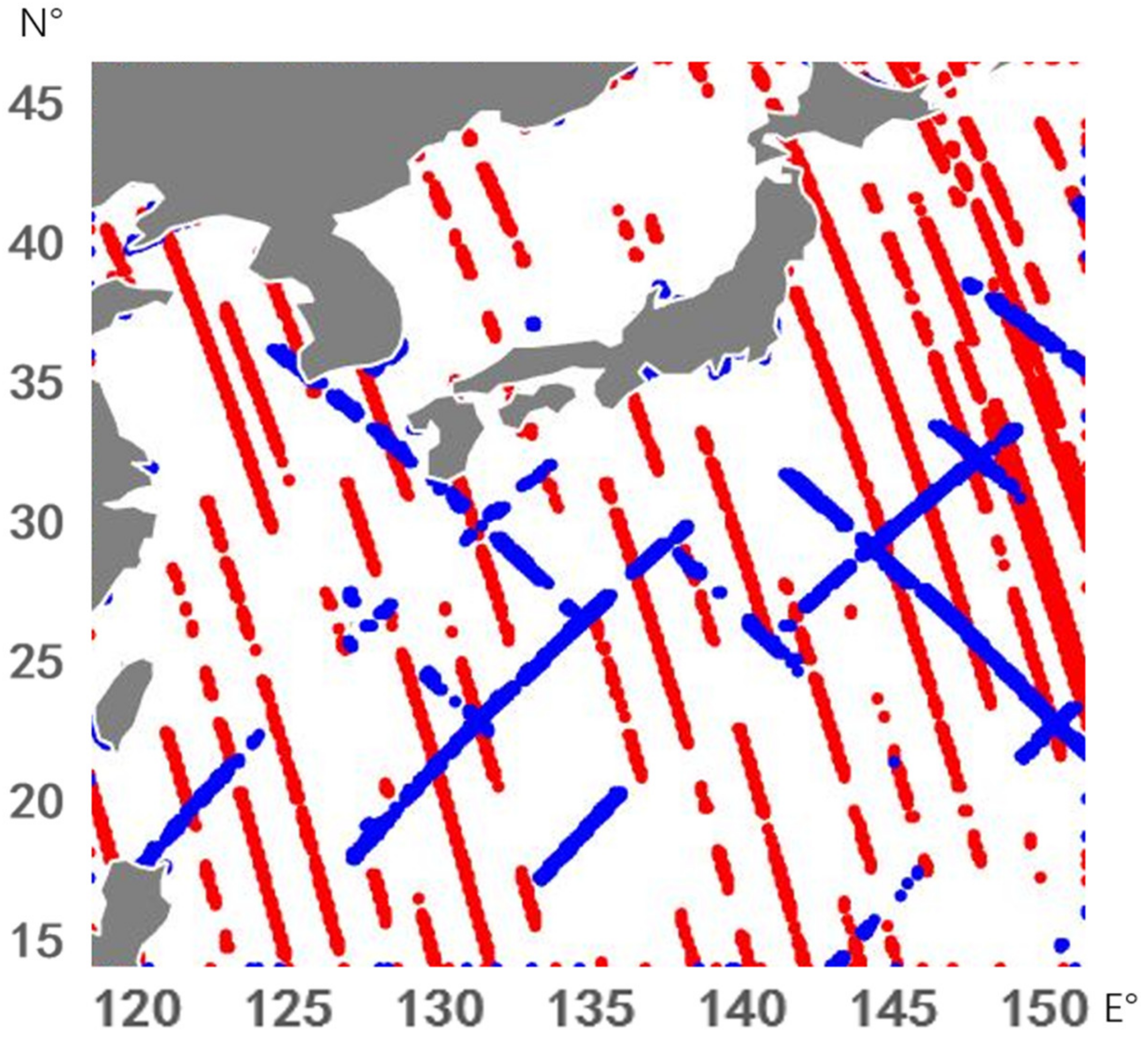
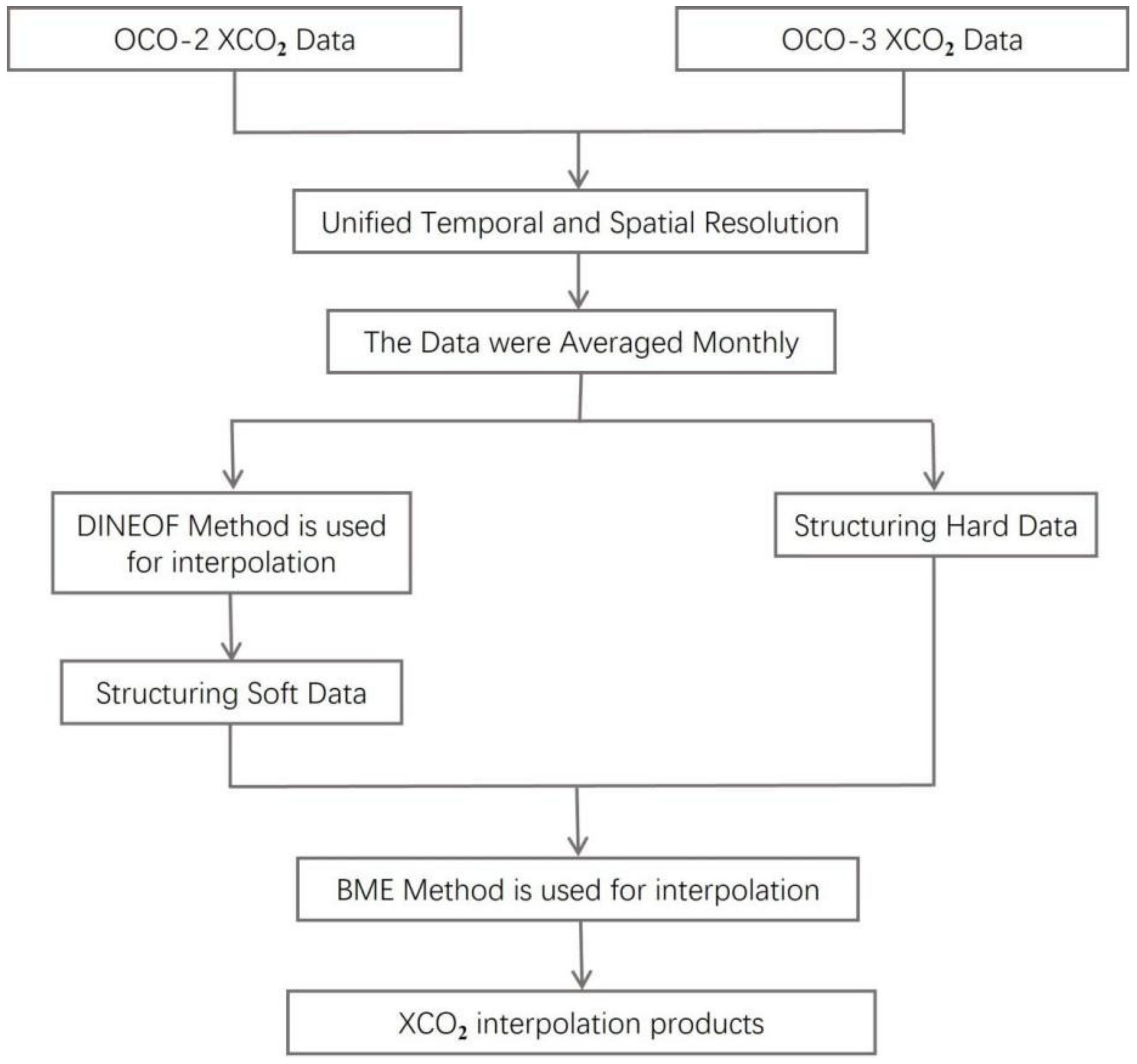
Simple fusion: the daily XCO2 data of OCO-2 and OCO-3 were directly and simply fused. First, the resolution of the two data was processed as a 0.1 latitude and longitude by averaging the data points in the same grid. Due to the great difference in the orbits of the two satellites, the data of the two satellites were rarely duplicated.
(c)
Monthly average processing: The time resolution of XCO2 data fused by OCO-2 and OCO-3 is daily, but the time range of this study is long. Therefore, the time resolution is adjusted to monthly, and the XCO2 data within the same grid point are averaged every month.

3.2. The DINEOF Method

DINEOF is an analysis method based on empirical orthogonal function analysis (EOF) for missing data interpolation and spatiotemporal modal extraction [21].
In the DINEOF method, X is assumed to be the original data matrix, where the dimension of Xmn is m × n (m > n), where m is the dimension of data Xmn in space, and n is the dimension of data Xmn in time. In this study, m refers to 90,000 spatial points in the study area (30°×30°), and n refers to 12-time instants (with unit month) units of the study. In the matrix X m n , each column represents all spatial points at the same time instant, and there are 90,000 spatial points corresponding to that time in each individual column, so the matrix X m n in this study has a total of 12 columns and 90,000 rows.
X m n = x 11 x 12 x 21 x 22 x 1 n x 2 n x m 1 x m 1 x m n
The space–time variable field X m n is decomposed into two parts: time function Z m n and space function V m m
X m n = V m m Z m n
The space function and the time function are respectively composed of m orthogonal space typical fields and corresponding time coefficients; that is, the decomposition of the time function and the decomposition of the space function must meet certain conditions:
v i T v j = 0 ,     i j 1 ,     i j z i T z j = 0 ,     i j λ j ,     i j z i T z j = 0 ,     i j λ j ,     i j
i , j = 1 , 2 m
After this premise is satisfied, the typical field in space point j can be expressed as:
v j = v 1 j , v 2 j v m j T
The time coefficient of space point i and time point t can be expressed as
z i t = p = 1 m v i p x p t
The space field at the space point k can be expressed as:
x k = v 1 z 1 k + v 2 z 2 k v m z m k
Let, A = X X T Then, according to the properties of space typical fields and corresponding time coefficients:
A = V Λ V T
The column vector of V is the feature vector of A, and the Λ is the eigenvalue matrix of A. Based on the decomposition principle of the EOF method mentioned above, the EOF calculation process of actual data can be summarized as the following six steps:
  • Determine the morphology of spatiotemporal variable field X m n ;
  • Find the covariance matrix of X m n : A = X X T ;
  • Calculate the eigenvalues and eigenvectors of matrix A;
  • The eigenvalues are arranged in ascending order to obtain the eigenvalue matrix, and the eigenvector matrix is changed accordingly;
  • Calculate time function;
  • Select the first N effective space typical fields and combine them with the corresponding time coefficients for modal calculation and output.
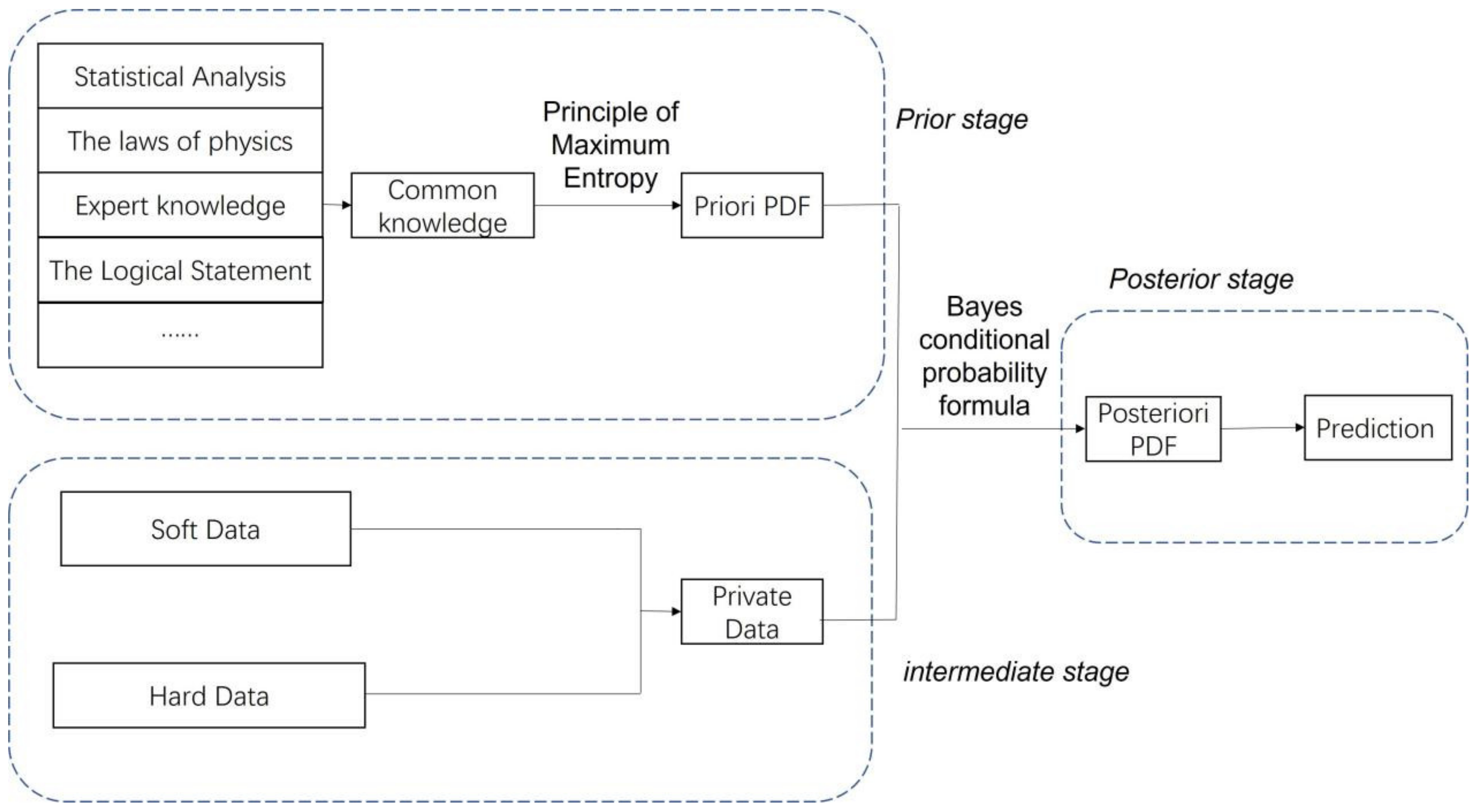
The EOF data reconstruction mentioned above is for complete data. However, a part of the actual data is missing to the extent that some additional processing must be performed on the missing dataset. Since EOF decomposition of large data volume is not affected by local minority changes, it can be used to obtain reconstructed values of missing regions through iterative EOF. Let matrix I include the set of not observed data points; when (i, j) ∈ I it means that the data at the space point i and time point j are missing. Then, EOF decomposition is performed for the spatiotemporal variable field X m n (refer to the EOF calculation steps above). The first N spatial typical fields are selected to reconstruct the whole space–time variable field
X m n = V m N Z N n
Then the unknown point X i j is updated immediately
x i j = v i 1 z 1 j + v i 2 z 2 j v i N Z N j
In this study, the DINEOF method is mainly used for the reconstruction of the missing data based on EOF for XCO2 data with large-scale missing data. The reconstructed data will be assimilated as soft data by the BME method, which is discussed in Section 3.3 below. In order to ensure the accuracy of the DINEOF results obtained within the time range considered in this study (January 2020 to December 2020), the DINEOF process was extended by one month before and after the time range. Data from December 2019 and January 2021 was also used in the DINEOF interpolation process. Finally, the DINEOF data results and the spatiotemporal modal images were obtained (see Section 4.2.1 for detailed analysis).

3.3. The BME Method

The BME method is a modern spatiotemporal geostatistics method that is a considerable improvement over the traditional geostatistics methods such as the Kriging method: for example, while Kriging techniques are limited to pure hard data interpolation, BME can integrate uncertain data from multiple sources in the spatiotemporal interpolation process to improve its accuracy; BME can be used in the case of nonlinear interpolation and non-Gaussian distributions, thus avoid some of the restrictions of the Kriging techniques. Several other advantages of BME have been discussed in detail in the relevant literature [16,28,29,30,31,32].
The three main stages of the BME method are as follows (Figure 2):
-
The prior stage considers the core or general knowledge base G–KB (including spatiotemporal covariance models, physical laws, and scientific theories). The general knowledge base in this study is the covariance function c X p , p (Equation (10)). The Spatiotemporal Random Field (STRF) X p is a collection of individual Random Variables (RV).
c X p , p = E X p E X p X p E X p
-
The intermediate stage involves the site-specific knowledge base (S-KB ‘Private data’ in Figure 2) consisting of hard (or accurate) data and soft data (i.e., data with inherent uncertainty, such as remote sensing data with low precision and information based on limited experience). In this study, the hard data were monthly average XCO2 data after the fusion of pretreated OCO-2 and OCO-3, whereas interpolating data processed by the DINEOF method will be used as soft data after removing the fusion data of OCO-2 and OCO-3.
-
The posterior stage integrates the two main knowledge bases above, G and S, to obtain the posterior probability density of the XCO2 spatiotemporal distribution or f G S = f K , where K = G S is the total KB expressed as the union of the core G and the site-specific S bases.
The above spatiotemporal XCO2 interpolation procedure is quantified in terms of the solution of the fundamental BME equations, as follows [17,32]:
d χ g g ¯ e μ · g = 0
d ψ χ e μ · g A f K = 0
where χ denotes the XCO2 concentrations across space–time, g is a vector of functions expressing mathematically the available core knowledge base G mentioned earlier; the g ¯ denotes the mean value of g ; the function ψ represents the available site-specific knowledge base S also mentioned earlier; the μ is a vector of coefficients representing the relative importance of each g -function ( μ · g denotes the inner product of the vectors g and μ , which are both functions of space–time); and A is a normalization parameter. Equations (11) and (12) can be solved with respect to the XCO2 probability law f K at all mapping points of interest (i.e., space–time points at which XCO2 interpolations are sought). Software libraries have been developed dealing with the solution of Equations (11) and (12) in real-world conditions, including BMElib, QuantumBME, and StarBME [33]. More technical details and physical interpretations of the basic BME equations above can be found in the relevant literature.

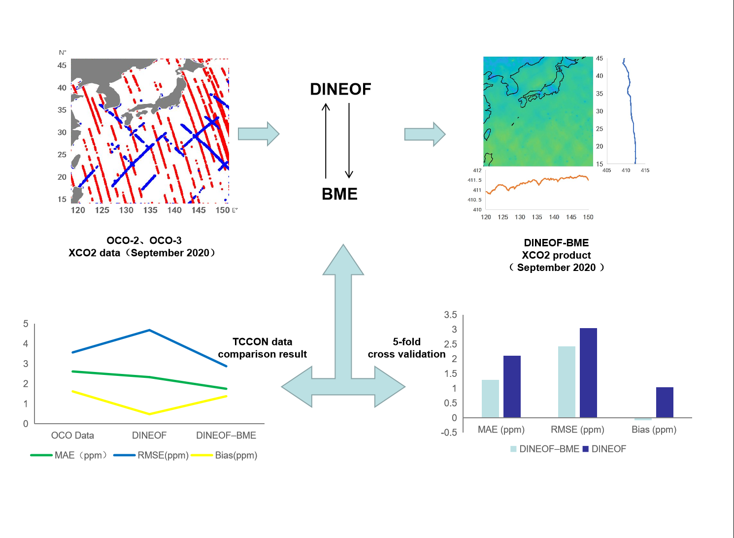
3.4. The Synthetic DINEOF–BME Interpolation Approach

In this study, the DINEOF and the BME methods are combined to interpolate the XCO2 remote sensing data of OCO-2 and OCO-3 satellites. The process can be roughly divided into four stages: (a) in the data pretreatment stage, the OCO-2 and OCO-3 data are merged into the OCO XCO2 dataset, the spatial resolution is processed to 0.1 decimal degree, and the monthly average is carried out; (b) the DINEOF stage, where the method is used to process the monthly averaged remote sensing data to produce the result data and spatiotemporal images; (c) the data structuring, where the remote sensing data processed by monthly average is directly constructed as hard data, while the data processed by DINEOF method excludes hard data points, and the rest is constructed as soft data; (d) the BME stage, where the method is used to interpolate the constructed hard data and soft data to obtain the final XCO2 product. The above process is outlined in Figure 3 below.

3.5. Validation and Comparison

In order to assess the accuracy of the synthetic DINEOF–BME method as well as the accuracy of the XCO2 interpolation results, this study implemented spatiotemporal image analysis and cross-validation analysis to verify the performance of the synthetic method, using TCCON as a comparison dataset. By calculating the mean deviation and root mean square error of TCCON XCO2 data with OCO-2 and OCO-3 satellite XCO2 data and using the synthetic DINEOF–BME interpolation framework, the product performance was analyzed.
EOF analyzes the data structure features in the matrix and extracts the feature quantity of the main data. It is also known as space–time modal decomposition in geostatistics and is a key data analysis element of the DINEOF method [33]. In this study, the temporal and spatial modes of OCO-2 and OCO-3 satellite XCO2 data were extracted for cartographic analysis.
The k-fold cross validation technique [34] was used to verify the interpolation accuracy of the BME method itself. In this study, taking the data volume and processing efficiency into consideration, the k value was set to five, and the time resolution was the month. In other words, in the hard data of 12 months from January to December 2020, the data of each month were randomly divided into five groups. In the cross-validation process, four of these groups were used as hard data for BME modeling purposes, and the other group was used for validation purposes. After all, five groups of data were validated, and the mean value of the five validation results was taken as the cross-validation result of that month.

4. Results

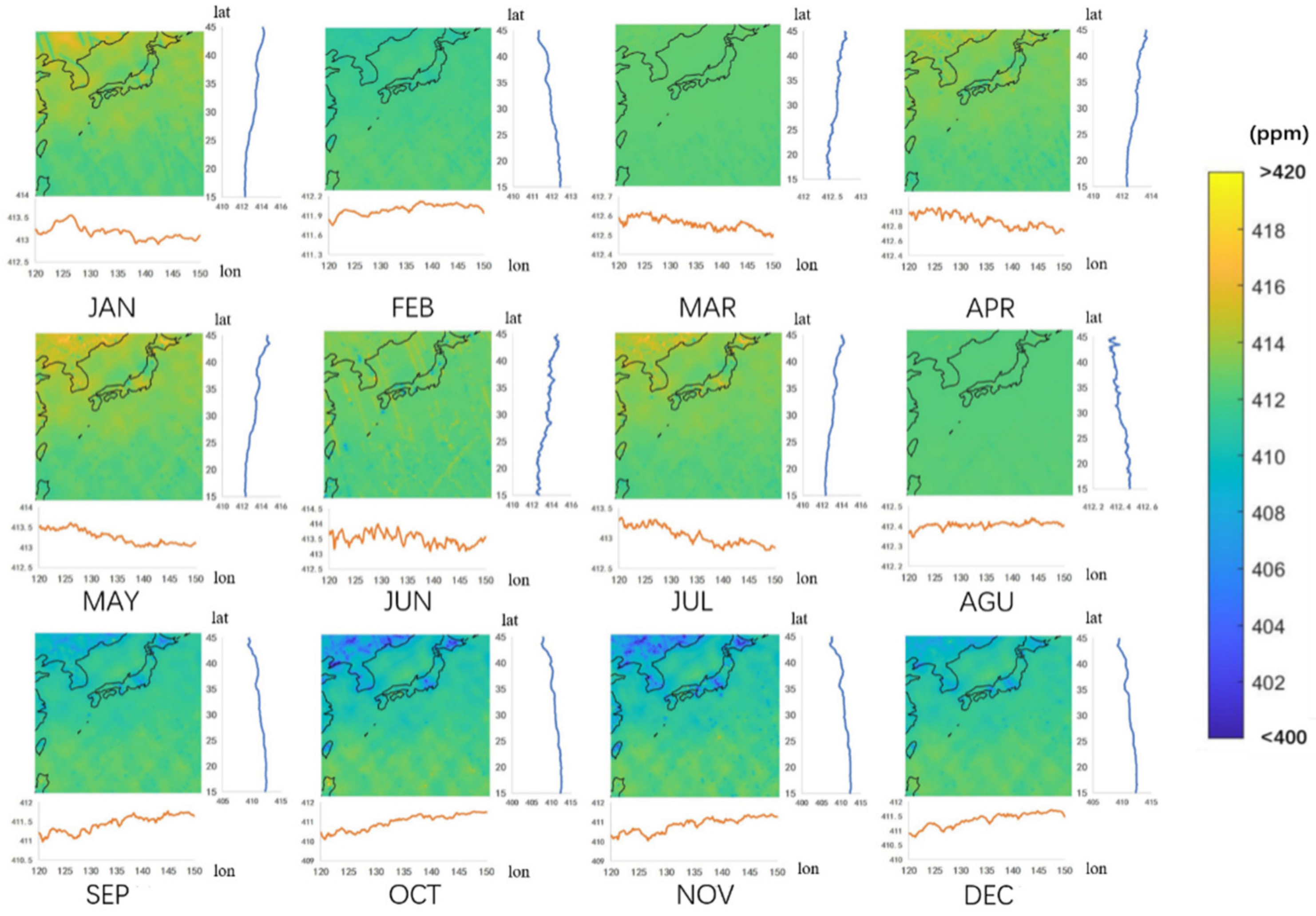
4.1. XCO2 Data Interpolation Results

Figure 4 shows the interpolation results of OCO-2 and OCO-3 XCO2 from January to December 2020 using the synthetic DINEOF–BME approach. In general, the overall quality of the products is high, and the product coverage rate reaches 100%. In addition, the product has high spatial resolution and perfect image detail. Figure 3 shows the distribution of XCO2 at the sea surface in that month and its change over time. According to the results of the twelve months shown in this figure, in the case of low air temperature from January to April and from October to December, the XCO2 is higher at the land edge and lower at the ocean. In the longitude direction, the higher the longitude, the lower the value, and in the zonal direction, the higher the latitude, the higher the value. The opposite is true for warmer temperatures from May to October. Thus, it can be seen that the XCO2 distribution exhibits obvious seasonal changes. During colder seasons, the regional XCO2 concentration decreases linearly with the distance between the region and the land. Conversely, in warmer seasons, the regional XCO2 concentration increases linearly with to the distance between the region and the land.

4.2. Comparison and Validation Analysis

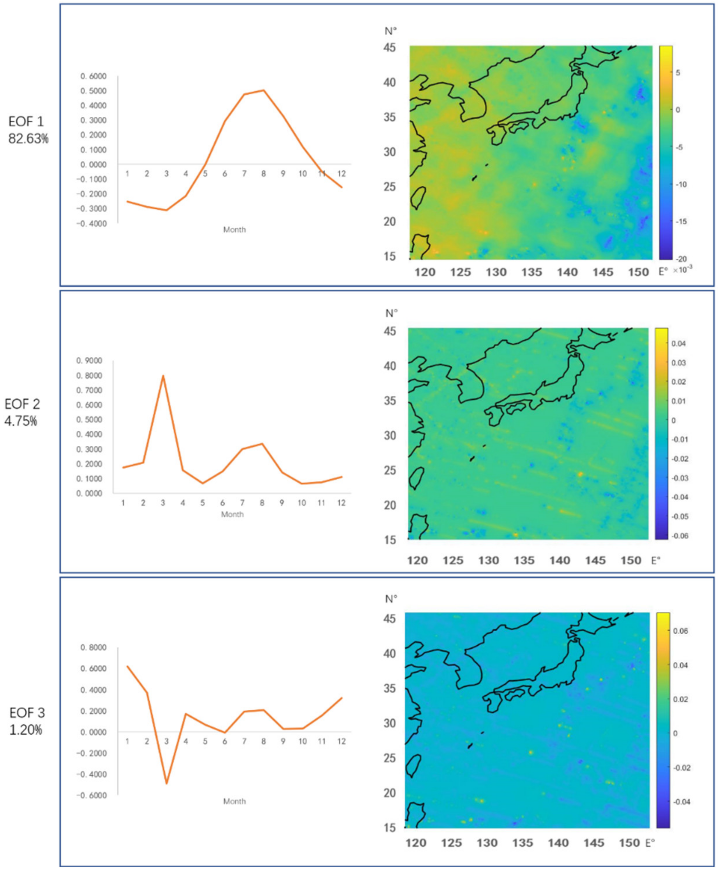
4.2.1. Spatiotemporal Model Analysis

The value of the EOF modal parameter represents its variance contribution rate, where the line chart of the time series represents the change of the whole study area over time, and the spatial modal chart represents the region that conforms to the change in the time series. If the spatial modal coefficient is positive, it means that the change of time series in this space conforms to the corresponding time mode. On the contrary, if the spatial modal coefficient is negative, it means that the time series change of this space is opposite to the corresponding time mode.
When using the three modes, DINEOF synthesized the XCO2 signal was the best, and the variance contribution rate reached 88.58%. The three patterns are shown in Figure 5, along with the corresponding variance contribution rates. The first temporal mode accounted for about 82.63% of the total variability and was an obvious seasonal signal, with a high value in summer and a low value in winter. The spatial distribution of the first EOF is generally positive in coastal areas and negative in offshore areas. In the coastal region, XCO2 is higher in summer and lower in winter, which is the same as the time series rule. In the far sea region, XCO2 is lower in summer and higher in winter, which is opposite to the time series rule. Preliminary analysis and previous studies show that human activity is the main reason for this phenomenon. That is, the more intense the human activity, the higher the XCO2 content in this area. Spatially, the findings of this study are consistent with these assessments.

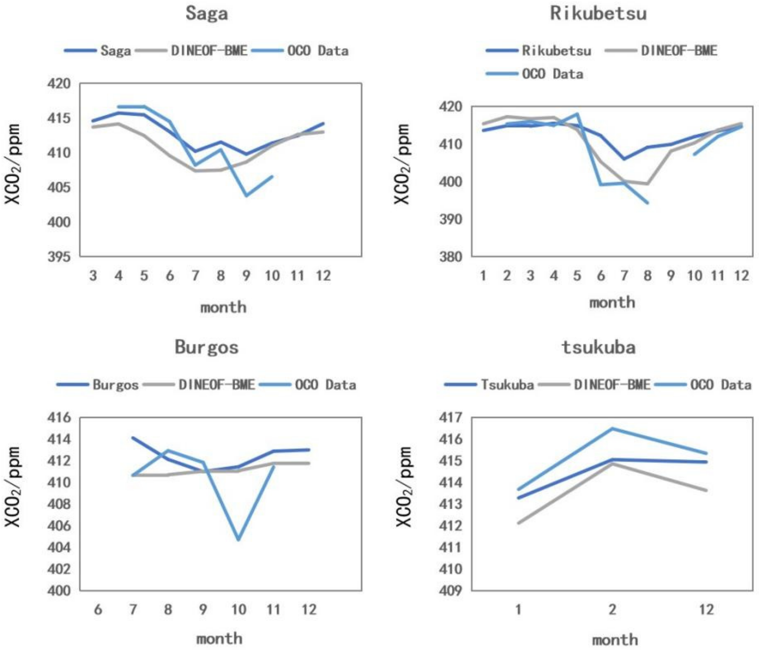
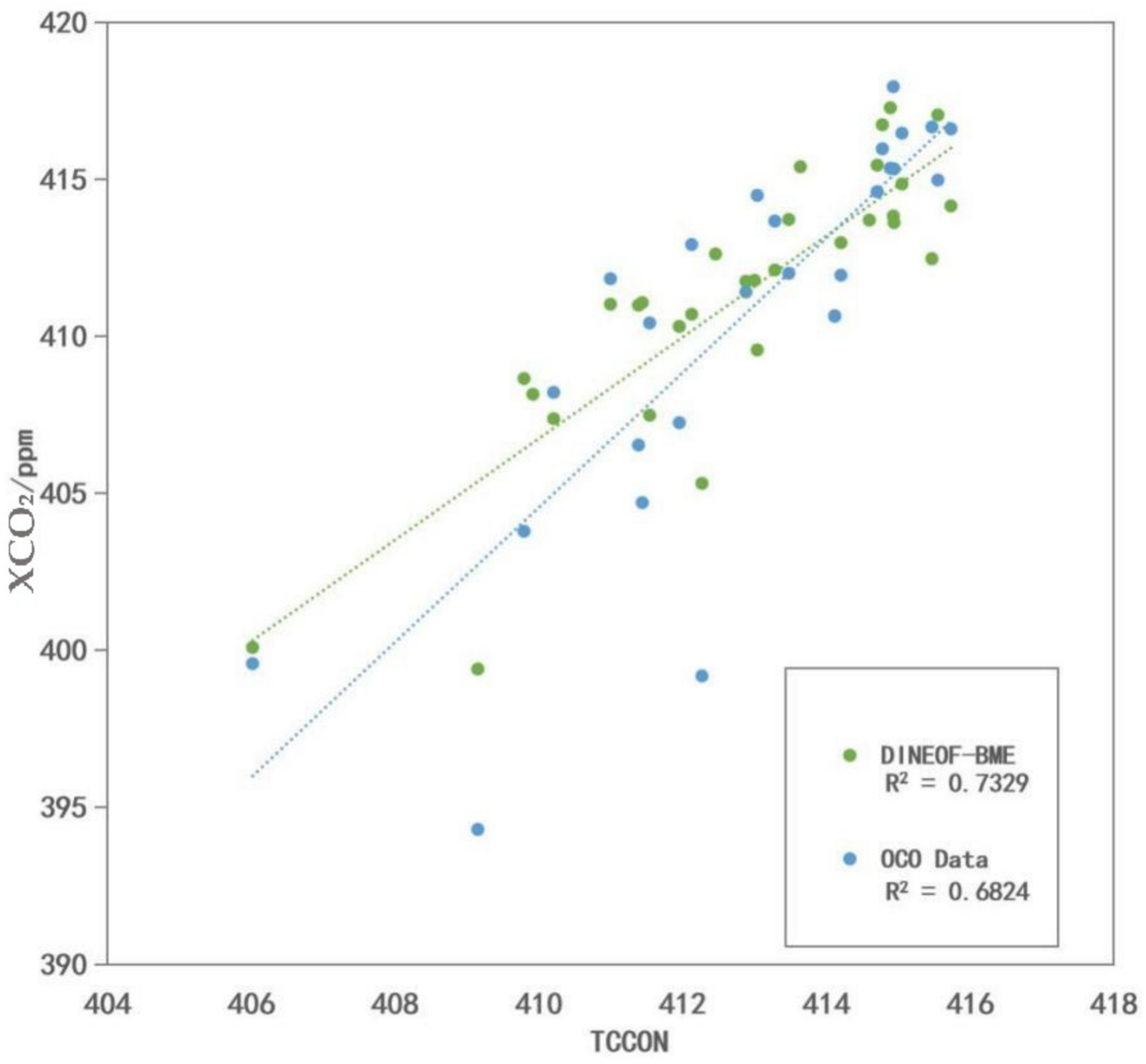
4.2.2. Cross Validation

In this study, the interpolation accuracy of the synthetic DINEOF–BME approach vs. the DINEOF technique alone was analyzed using a five-fold cross-validation method. The mean absolute error, mean square error, and root mean square error of 60 groups of cross-validation data were calculated for a total of 12 months in 2020, and then the mean value was processed. The results are shown in Table 1. For the synthetic DINEOF–BME approach, the MAE is 1.285 ppm, RMSE is 2.422 ppm, Bias is −0.085 ppm, and for the DINEOF technique, the MAE is 2.106 ppm, RMSE is 3.046 ppm, Bias is 1.035 ppm. It can be seen that the cross-validation result of the synthetic DINEOF–BME approach is better than that of using only the DINEOF technique, which implies that the proposed synthetic approach combining the two methods produces more accurate results.

4.2.3. Comparative Analysis

In this study, TCCON XCO2 measured dataset was used to compare with OCO XCO2 data and DINEOF interpolation XCO2 products with the BME method from MAE and RMSE. The overall situation is shown in Table 2.
The coverage of the XCO2 products obtained by the synthetic DINEOF–BME interpolation reached the optimal 100% level in the study area, which is 84% higher than the 16% of OCO data, thus, demonstrating a perfect performance of the synthetic DINEOF–BME approach in this respect.
The mean MAE of the synthetic DINEOF–BME interpolation products, the DINEOF products, and the OCO data matched with TCCON data were 1.751 ppm, 2.334 ppm, and 2.616 ppm, respectively. The RMSE values were 2.877 ppm, 4.682 ppm, and 3.566 ppm, and the Bias values were 1.379 ppm, 0.483 ppm, and 1.622 ppm, respectively.
Figure 6 shows the measured XCO2 data obtained by TCCON at four stations in the study area and the line chart of comparison with OCO XCO2 data and DINEOF–BME interpolation XCO2 data. In addition to the above-mentioned average error of DINEOF–BME, interpolation products are obviously better than OCO data; from the perspective of time, DINEOF–BME interpolation products are also more consistent with the changing trend of measured data. Similarly, as shown in Figure 7, the R2 matching values of TCCON measured XCO2 data, OCO XCO2 data, and DINEOF–BME interpolation XCO2 data are 0.733 and 0.682, respectively, which also proves that DINEOF–BME products have higher matching degree.

5. Discussion

5.1. Methodology

In this study, a synthetic spatiotemporal interpolation framework with the BME method as the dominant component and DINEOF as the auxiliary component was constructed. The synthesis of these two methods gives full play to their own characteristics, and it also achieves fruitful cooperation between them.
DINEOF method has been successfully applied to the study of sea surface chlorophyll-a, sea surface salinity, sea surface temperature, and other ocean data [35,36]. According to its description in Section 3.2, the DINEOF method systematically decomposed and reconstructed spatiotemporal data based on the characteristics of the data field. Although this process would lead to the loss of a large amount of effective data information, whereas only the spatiotemporal characteristics of data would be retained, it can greatly improve the interpolation data coverage. As is shown in Figure 8 below, in this study, the DINEOF method has improved the average XCO2 data coverage rate of OCO-2 and OCO-3 from 16% to 97%, whereas the BME method has further improved the coverage rate to 100%. The coverage of the DINEOF method does not reach 100% because this method cannot provide output for the 3% of cases where no data are available at sufficiently close times and locations for the spatiotemporal interpolation. It is clear that the task of improving coverage is primarily accomplished by the DINEOF method. In this setting, the DINEOF interpolation results can be further improved, thanks to the strong theoretical basis and inclusiveness of the BME method.
As the most advanced geostatistical spatiotemporal interpolation method currently in use, the BME method is a nonlinear interpolator, in general, that accounts for non-Gaussian distributions too. Compared to traditional interpolation methods such as the various Kriging and inverse weighted distance techniques, BME has a more sound theoretical support and can optimize the use and retention of various data information sources to improve interpolation accuracy. As more kinds and types of marine data are gradually acquired, geostatistical methods are increasingly applied to marine data processing and scientific research [18,19]. In this study, the BME’s ability to absorb uncertain soft data in spatiotemporal interpolation plays a key role [37,38,39]. For example, some other models (such as sample regression and vector regression) have been used to generate soft data for BME interpolation purposes [40,41]. In this study, instead, the DINEOF interpolation results in the form of probability distributions were used as soft data for BME interpolation, which effectively allowed the two methods to complement each other in order to obtain more accurate spatiotemporal interpolation results.
The core advantage of the study framework used in the present study lies in the powerful generalizability and strong inclusiveness of the BME method, which enable it to (a) assimilate different types of XCO2 data and (b) be combined with various techniques (such as DINEOF) to improve spatiotemporal interpolation accuracy. Such a framework has not been considered in previous studies of XCO2 interpolation studies. Instead, various types of geostatistical Kriging techniques have been used. For example, the spatial Kriging technique has been widely used in XCO2 interpolation research (NIES GOSAT PROJECT 2011). There are also related XCO2 interpolation studies involving an improved variogram modeling in Kriging interpolation [11,12]. Moreover, the fixed-rank Kriging method (FRK) has been used in XCO2 interpolation [42]. Although these studies can improve the ordinary Kriging techniques, they still cannot fully utilize the complete information provided by the XCO2 datasets. Similarly, mainstream Kriging techniques have also been used to fuse GOSAT and SCIMACHY XCO2 datasets [43]. However, unlike BME, these Kriging techniques cannot take into account data uncertainties, which need to be processed by other techniques before interpolation is implemented. In sum, the proposed framework with BME theory at its core can maximize the assimilated information in the various forms of uncertain data and systematically integrate other powerful methods as well (such as DINEOF).

5.2. Product Analysis

Analysis of XCO2 products is mainly concerned with coverage and accuracy.
In terms of coverage, current XCO2 acquisition tools mainly rely on carbon satellites and measured data. Any kind of measured dataset basically cannot achieve large-scale coverage. As is shown in Figure 1, the data obtained by carbon satellites currently in orbit (such as OCO-2, OCO-3, and GOSAT) display obvious bands in global images [44]. Unlike this kind of data, in the case of, e.g., sea surface temperature (SST) and sea surface salinity (SSS), their coverage rate in the global ocean is very low, and there is a very large gap. On the other hand, the XCO2 products obtained in this study have achieved 100% coverage in the region, with excellent performance.
In terms of accuracy, the matter mainly involves two aspects: the method and the data itself. The part about the method has been explained in detail in Section 5.1, so we do not elaborate further here. As regards the data, the spatial resolution of OCO-2 data is about 1.3 km × 2.3 km, and that of OCO-3 data is about 1.6 km×2.2 km, which is better than that of most carbon satellites [7,24,44,45,46,47]. Table 3 shows the spatial resolution comparison of some carbon satellites. As is well known, the higher the spatial resolution, the finer the information. The image produced in this study is a fusion of OCO-2 and OCO-3 XCO2 data and is plotted at a spatial resolution of a 0.1 latitude and longitude, yielding very fine image results. In addition, relevant studies have shown that the XCO2 data accuracy is related to aerosol or surface reflectance interference [8,48,49,50]. Therefore, the XCO2 change is smaller than that of land [50]. Lastly, the stronger the spatiotemporal data correlation is, the more accurate the BME interpolation results will be.

5.3. Prospects and Expectations

This study explored a synthetic interpolation framework that combined the DINEOF and BME methods and confirmed the positive effects of this synthesis in the spatiotemporal interpolation context. The results showed that the interpolation product performs very well in terms of coverage and accuracy, indicating the power of the synthetic approach. In addition, this study addressed the issue of interpolation relying only on spatiotemporal distance and ignoring spatiotemporal strongly correlated features by noticing that the BME method provides a solution to this problem by means of its strong scalability and inclusiveness features. Using diverse soft data, as well as combining other related techniques with the BME method, are issues that are worthy of further study. High-quality XCO2 interpolation products of sea surfaces were also obtained in this study. Indeed, it is of great significance to simultaneously satisfy the high coverage rate and high accuracy of sea surface XCO2 data.
At present, XCO2 studies are more focused on the land but less on the ocean. However, XCO2 in the ocean region is closely related to sea-air CO2 flux [51]. XCO2 has a significant impact on marine climate change, ocean acidification, marine fisheries, and other related fields [52,53,54]. High-quality XCO2 data could be potentially applied to the construction of relevant data and the analysis of related fields, laying a good foundation for future research. In addition, the BME interpolation of XCO2 products could be of great help in the acquisition of large-scale XCO2 data by referring to the synthetic approach proposed in this study and further analyzing the temporal and spatial variation rules (such rules include the relationship between XCO2 in the ocean region and human activities in coastal areas, the correlation between XCO2 in the ocean region and seasonal variation, and latitude and longitude variation), or other relevant analysis and research issues based on XCO2 data.
In addition, considering the computational cost and other issues, this study only performs interpolation on small spatial and temporal scales. Future work will focus on improving the efficiency of the software, significantly reducing the computational cost, and applying the developed method to explore the spatial and temporal distribution and characteristics of global XCO2.

6. Conclusions

In this paper, the empirical orthogonal function interpolation (DINEOF) method and the Bayesian Maximum Entropy (BME) methods were combined to interpolate XCO2 data of OCO-2 and OCO-3 from January to December 2020 in the geographical range of 15-45°N and 120-150°E. The spatiotemporal modal analysis verified that the OCO-2 and OCO-3 XCO2 data have obvious spatiotemporal characteristics. The BME interpolation accuracy was evaluated by using a five-fold cross-validation method. The results showed that the MAE value is 1.29 ppm, and the RMSE value is 2.42 ppm. In addition, based on the measured XCO2 data provided by TCCON, OCO-2 and OCO-3 data were compared with the synthetic DINEOF–BME interpolation products. The results showed that the interpolation products increased the coverage of OCO-2 and OCO-3 products from 16% to 100%. As regards matching, the MAE, RMSE, and R2 values of OCO-2 and OCO-3 data and TCCON measured data were found to be equal to 2.616 ppm, 3.566 ppm, and 0.682, respectively. The MAE, RMSE, and R2 values of the interpolated products and TCCON data were 1.751 ppm, 2.877 ppm, and 0.733, respectively. In addition to the coverage of DINEOF–BME interpolation products, MAE, RMSE, and R2 performance parameters are also better than OCO data, indicating that DINEOF–BME interpolation products have smaller errors and better data stability. In addition, the present work confirmed the feasibility of combining the DINEOF with the BME methods. Moreover, the BME inclusiveness was further demonstrated based on its strong theoretical support. By integrating other kinds of techniques and information sources in the major BME framework, better interpolation results are anticipated in the future.

Author Contributions

Methodology, Y.J.; validation, Y.J. and Z.G.; formal analysis, Y.J. and Z.G.; resources, Y.J.; data curation, Y.J.; writing—original draft preparation, Y.J. and Z.G.; writing—review and editing, G.C. and J.H.; project administration, G.C. and J.W. All authors have read and agreed to the published version of the manuscript.

Funding

This research was funded by the China Postdoctoral Science Foundation, Junyu He, grant number 2020M681825 and The APC was funded by National Natural Science Foundation of China, George Christakos, grant number NSFC 42171398.

Data Availability Statement

XCO2 remote sensing data: The Orbiting Carbon Observatory 3 (OCO-3) XCO2 data: https://oco2.gesdisc.eosdis.nasa.gov/data/OCO3_DATA/OCO3_L2_Lite_FP.10.4r/2020/ (accessed on 1 December 2021). The Orbiting Carbon Observatory 2 (OCO-2) XCO2 data: https://oco2.gesdisc.eosdis.nasa.gov/data/OCO2_DATA/OCO2_L2_Lite_FP.10r/2020/ (accessed on 1 December 2021). XCO2 measurements data: TCCON: https://data.caltech.edu/records/20140. (accessed on 1 December 2021).

Conflicts of Interest

The authors declare no conflict of interest.

References

  1. Grubler, A. IPCC Fifth Assessment Report. Weather 2014, 68, 310. [Google Scholar]
  2. Liu, H.; Rodriguez, G. Human Activities and Global Warming: A Cointegration Analysis. Environ. Model. Softw. 2003, 20, 761–773. [Google Scholar] [CrossRef]
  3. Robinson, I.S. Discovering the Ocean from Space: The Unique Applications of Satellite Oceanography; Springer: Berlin/Heidelberg, Germany, 2010. [Google Scholar]
  4. Solomon, S. Working Group 1 contribution to the IPCC fifth assessment report. In Climate Change 2013: The Physical Science Basis; Cambridge University Press: Cambridge, UK, 2007. [Google Scholar]
  5. Akihiko, K.; Hiroshi, S.; Masakatsu, N.; Takashi, H. Thermal and near infrared sensor or carbon observation Fourier-transform spectrometer on the Greenhouse Gases Observing Satellite for greenhouse gases monitoring. Appl. Opt. 2009, 48, 6716–6733. [Google Scholar] [CrossRef]
  6. Frankenber, C.; Pollock, R.; Lee, R.A.M.; Rosenberg, R.; Blavier, J.-F.; Crisp, D.; O’Dell, C.W. The Orbiting Carbon Observatory (OCO-2): Spectrometer performance evaluation using pre-launch direct sun measurements. Atmos. Meas. Tech. 2015, 8, 301–313. [Google Scholar] [CrossRef]
  7. Yokota, T.; Yoshida, Y.; Eguchi, N.; Ota, Y.; Tanaka, T.; Watanabe, H.; Maksyutov, S. Global Concentrations of CO2 and CH4 Retrieved from GOSAT: First Preliminary Results. Sola 2009, 5, 160–163. [Google Scholar] [CrossRef]
  8. Houweling, S.; Hartmann, W.; Aben, I.; Schrijver, H.; Skidmore, J.; Roelofs, G.J.; Breon, F.M. Evidence of systematic errors in sciamachy-observed CO2 due to aerosols. Atmos. Chem. Phys. 2005, 5, 3003–3013. [Google Scholar] [CrossRef]
  9. Velazco, V.A.; Buchwitz, M.; Bovensmann, H.; Reuter, M.; Schneising, O.; Heymann, J.; Krings, T.; Krings, T.; Burrows, J.P. Towards space based verification of CO2 emissions from strong localized sources: Fossil fuel power plant emissions as seen by a CarbonSat constellation. Atmos. Meas. Tech. Discuss. 2011, 4, 5147–5182. [Google Scholar] [CrossRef]
  10. Cai, Z.N.; Liu, Y.; Yang, D.X. Analysis of XCO2 retrieval sensitivity using simulated Chinese Carbon Satellite (TanSat) measurements. Sci. China Earth Sci. 2014, 57, 1919–1928. [Google Scholar] [CrossRef]
  11. Guo, L.; Lei, L.; Zeng, Z.; Zou, P.; Liu, D.; Zhang, B. Evaluation of Spatio-Temporal Variogram Models for Mapping Xco(2) Using Satellite Observations: A Case Study in China. IEEE J. Sel. Top. Appl. Earth Obs. Remote Sens. 2015, 8, 376–385. [Google Scholar] [CrossRef]
  12. Zeng, Z.; Lei, L.; Hou, S.; Li, L. A spatio-temporal interpolation approach for the FTS SWIR product of XCO2 data from GOSAT. In Proceedings of the Geoscience & Remote Sensing Symposium IEEE, Munich, Germany, 22–27 July 2012. [Google Scholar]
  13. Azcarate, A.A.; Barth, A.; Beckers, J.M.; Weisberg, R.H. Multivariate reconstruction of missing data in sea surface temperature, chlorophyll, and wind satellite fields. J. Geophys. Res. Ocean. 2007, 112, C03008. [Google Scholar] [CrossRef]
  14. Azcarate, A.A.; Barth, A.; Sirjacobs, D.; Lenartz, F.; Beckers, J.M. Data Interpolating Empirical Orthogonal Functions (DINEOF): A tool for geophysical data analyses. Mediterr. Mar. Sci. 2011, 12, 1–5. [Google Scholar] [CrossRef] [Green Version]
  15. Christakos, G. A Bayesian/maximum-entropy view to the spatial estimation problem. Math. Geol. 1990, 22, 763–777. [Google Scholar] [CrossRef]
  16. Christakos, G. Modern Spatiotemporal Geostatistics; Oxford University Press: New York, NY, USA, 2000. [Google Scholar]
  17. He, J.; Kolovos, A. Bayesian maximum entropy approach and its applications: A review. Stoch. Environ. Res. Risk Assess. 2017, 32, 859–877. [Google Scholar] [CrossRef]
  18. Lang, Y.; Christakos, G. Ocean pollution assessment by integrating physical law and site-specific data. Environmetrics 2019, 30, e2547. [Google Scholar] [CrossRef]
  19. He, J.; Chen, Y.; Wu, J.; Stow, D.A.; Christakos, G. Space-time chlorophyll-a retrieval in optically complex waters that accounts for remote sensing and modeling uncertainties and improves remote estimation accuracy. Water Res. 2020, 171, 115403. [Google Scholar] [CrossRef] [PubMed]
  20. He, M.; He, J.; Christakos, G. Improved Space-Time Sea Surface Salinity Mapping in Western Pacific Ocean Using Contingogram Modeling. Stoch. Environ. Res. Risk Assess. 2020, 34, 355–368. [Google Scholar] [CrossRef]
  21. Pearson, K. LIII. On lines and planes of closest fit to systems of points in space. Philos. Mag. 1901, 2, 559–572. [Google Scholar] [CrossRef]
  22. Azcarate, A.A.; Barth, A.; Rixen, M.; Beckers, J.M. Reconstruction of incomplete oceanographic data sets using empirical orthogonal functions: Application to the Adriatic Sea surface temperature. Ocean Model. 2005, 9, 325–346. [Google Scholar] [CrossRef]
  23. Crisp, D.; Pollock, H.R.; Rosenberg, R.; Chapsky, L.; Wunch, D. The on-orbit performance of the Orbiting Carbon Observatory-2 (OCO-2) instrument and its radiometrically calibrated products. Atmos. Meas. Tech. 2017, 10, 1–45. [Google Scholar] [CrossRef]
  24. Taylor, T.E.; Eldering, A.; Merrelli, A.; Kiel, M.; Yu, S. OCO-3 early mission operations and initial (vEarly) XCO2 and SIF retrievals. Remote Sens. Environ. 2020, 251, 112032. [Google Scholar] [CrossRef]
  25. Eldering, A.; Taylor, T.E.; O’Dell, C.W.; Pavlick, R. The OCO-3 mission: Measurement objectives and expected performance based on 1 year of simulated data. Atmos. Meas. Tech. 2019, 12, 2341–2370. [Google Scholar] [CrossRef] [Green Version]
  26. Wunch, D.; Toon, G.C.; Blavier, J.-F.L.; Washenfelder, R.A.; Notholt, J.; Connor, B.J.; Griffith, D.W.T.; Sherlock, V.; Wennberg, P.O. The Total Carbon Column Observing Network. Philos. Trans. R. Soc. A Math. Phys. Eng. Sci. 2011, 369, 2087–2112. [Google Scholar] [CrossRef] [PubMed]
  27. Wunch, D.; Toon, G.C.; Blavier, J.F.L.; Washenfelder, R.A.; Notholt, J.; Connor, B.J.; Griffith, D.W.; Sherlock, V.; Wennberg, P.O. The Total Carbon Column Observing Network’s GGG2014 Data Version, Pasadena, California. Philos. Trans. R. Soc. A Math. Phys. Eng. Sci. 2015, 369, 2087–2112. [Google Scholar] [CrossRef] [PubMed]
  28. Christakos, G. Spatiotemporal Random Fields: Theory and Applications; Elsevier: Amsterdam, The Netherlands, 2017. [Google Scholar]
  29. Bogaert, P.; Christakos, G.; Jerrett, M.; Yu, H.L. Spatiotemporal modelling of ozone distribution in the State of California. Atmos. Environ. 2009, 43, 2471–2480. [Google Scholar] [CrossRef]
  30. Gao, S.G.; Zhu, Z.L.; Liu, S.M.; Jin, R.; Yang, G.C.; Tan, L. Estimating the spatial distribution of soil moisture based on Bayesian maximum entropy method with auxiliary data from remote sensing (SCI). Int. J. Appl. Earth Obs. Geoinf. 2014, 32, 54–66. [Google Scholar]
  31. Lee, S.J.; Balling, R.; Gober, P. Bayesian maximum entropy mapping and the soft data problem in urban climate research. Ann. Assoc. Am. Geogr. 2008, 98, 309–322. [Google Scholar] [CrossRef]
  32. Li, X.; Li, P.; Zhu, H. Coal seam surface modeling and updating with multisource data integration using Bayesian Geostatistics. Eng. Geol. 2013, 164, 208–221. [Google Scholar] [CrossRef]
  33. Yu, H.L.; Kolovos, A.; Christakos, G.; Chen, J.C.; Warmerdam, S.; Dev, B. Interactive spatiotemporal modelling of health systems: The SEKS-GUI framework. Stoch. Environ. Res. Risk Assess. 2007, 21, 555–572. [Google Scholar] [CrossRef]
  34. Kohavi, R. A study of cross-validation and bootstrap for accuracy estimation and model selection. In Proceedings of the International Joint Conference on Artificial Intelligence, Montreal, QC, Canada, 20–25 August 1995; Morgan Kaufmann Publishers Inc.: Burlington, MA, USA, 1995. [Google Scholar]
  35. Beckers, J.M.; Barth, A.; Azcarate, A.A. DINEOF reconstruction of clouded images including error maps. Application to the Sea-Surface Temperature around Corsican Island. Ocean Sci. 2006, 2, 183–199. [Google Scholar] [CrossRef]
  36. Azcarate, A.A.; Barth, A.; Parard, G.; Beckers, J. Analysis of SMOS sea surface salinity data using DINEOF. Remote Sens. Environ. 2016, 180, 137–145. [Google Scholar] [CrossRef]
  37. Bogaert, P.; D’Or, D. Estimating Soil Properties from thematic Soil Maps: The Bayesian Maximum Entropy Approach. Soil Sci. Soc. Am. J. 2002, 66, 1492–1500. [Google Scholar] [CrossRef]
  38. Christakos, G. On the assimilation of uncertain physical knowledge bases: Bayesian and non-Bayesian techniques. Adv. Water Resour. 2002, 25, 1257–1274. [Google Scholar] [CrossRef]
  39. Christakos, G.; Kolovos, A.; Serre, M.L.; Vukovich, F. Total ozone mapping by integrating databases from remote sensing instruments and empirical models. Geosci. Remote Sens. IEEE Trans. 2004, 42, 991–1008. [Google Scholar] [CrossRef]
  40. Jiang, Q.; He, J.; Wu, J.; Hu, X.; Ye, G.; Christakos, G. Assessing the Severe Eutrophication Status and Spatial Trend in the Coastal Waters of Zhejiang Province (China). Limnol. Oceanogr. 2018, 64, 3–17. [Google Scholar] [CrossRef]
  41. He, J.; Christakos, G.; Wu, J.; Li, M.; Leng, J. Spatiotemporal BME Characterization and Mapping of Sea Surface Chlorophyll in Chesapeake Bay (USA) Using Auxiliary Sea Surface Temperature Data. Sci. Total Environ. 2021, 794, 148670. [Google Scholar] [CrossRef] [PubMed]
  42. Cong, Z.; Shi, R.; Wei, G. Interpolation of XCO2 retrieved from GOSAT in China using fixed rank kriging. In Proceedings of the SPIE-The International Society for Optical Engineering, San Diego, CA, USA, 24 September 2013; Volume 8869, pp. 281–291. [Google Scholar] [CrossRef]
  43. Jing, Y.; Shi, J.; Wang, T. Mapping global land XCO2 from measurements of GOSAT and SCIAMACHY by using kriging interpolation method. In Proceedings of the IGARSS 2014-2014 IEEE International Geoscience and Remote Sensing Symposium, Quebec City, QC, Canada, 13–18 July 2014. [Google Scholar]
  44. Liang, A.; Gong, W.; Ge, H.; Xiang, C. Comparison of Satellite-Observed XCO2 from GOSAT, OCO-2, and Ground-Based TCCON. Remote Sens. 2017, 9, 1033. [Google Scholar] [CrossRef]
  45. Du, S.; Liu, L.; Liu, X.; Zhang, X.; Bi, Y.; Zhang, L. Retrieval of global terrestrial solar-induced chlorophyll fluorescence from TanSat satellite. Sci. Bull. 2018, 22, 1502–1512. [Google Scholar] [CrossRef]
  46. Pillai, D.; Buchwitz, M.; Bovensmann, H.; Reuter, M.; Burrows, J. Inferring source and sink of atmospheric CO2 at high-resolution from space: A mesoscale modeling approach using inverse technique. In Proceedings of the EGU General Assembly Conference Abstracts, Vienna, Austria, 7–12 April 2012. [Google Scholar]
  47. Wang, T.; Shi, J.; Jing, Y.; Zhao, T.; Ji, D.; Xiong, C. Combining XCO2 Measurements Derived from SCIAMACHY and GOSAT for Potentially Generating Global CO2 Maps with High Spatiotemporal Resolution. PLoS ONE 2012, 9, e0148152. [Google Scholar] [CrossRef]
  48. Aben, I.; Hasekamp, O.; Hartmann, W. Uncertainties in the space-based measurements of CO2 columns due to scattering in the Earth’s atmosphere. J. Quant. Spectrosc. Radiat. Transf. 2007, 104, 450–459. [Google Scholar] [CrossRef]
  49. Butz, A.; Hasekamp, O.P.; Frankenberg, C.; Aben, I. Retrievals of atmospheric CO2 from simulated space-borne measurements of backscattered near-infrared sunlight: Accounting for aerosol effects. Appl. Opt. 2009, 48, 3322–3336. [Google Scholar] [CrossRef]
  50. Guerlet, S. Impact of aerosol and thin cirrus on retrieving and validating XCO2 from GOSAT shortwave infrared measurements. J. Geophys. Res. Atmos. 2013, 118, 4887–4905. [Google Scholar] [CrossRef] [Green Version]
  51. Takagi, H. Characteristics of multi-year-long regional CO2 fluxes estimated from GOSAT XCO2 retrievals. In Agu Fall Meeting Abstracts; American Geophysical Union: Washington, DC, USA, 2015. [Google Scholar]
  52. Camy-Peyret, C.; Bureau, J.; Payan, S. Evolution of SST and XCO2 in the summer ice free Arctic Ocean: Is IASI able to contribute to climate change studies? In Proceedings of the 4th IASI International Conference, Antibes Juan-Les-Pins, France, 20 April 2016. [Google Scholar]
  53. Jiang, X. Carbon Dioxide Induced Ocean Climatic Change and Tracer Experiment with an Atmosphere-Ocean General Circulation Model. Ph.D. Thesis, University of Illinois, Chicago, IL, USA, 1991. [Google Scholar]
  54. Ferrari MC, O.; Mccormick, M.I.; Watson, S.-A.; Meekan, M.G.; Munday, P.L.; Chivers, D.P. Predation in High CO2 Waters: Prey Fish from High-Risk Environments are Less Susceptible to Ocean Acidification. Integr. Comp. Biol. 2017, 57, 55. [Google Scholar] [CrossRef] [PubMed] [Green Version]
Figure 1. The Trajectories of OCO-2 (red) and OCO-3 (blue) Satellites during September.
Remotesensing 14 04422 g001
Figure 2. Workflow of the BME analysis.
Remotesensing 14 04422 g002
Figure 3. Construction Chart of the Study.
Remotesensing 14 04422 g003
Figure 4. Monthly Interpolation Results of XCO2 from January to December 2020(The orange line graph at the bottom of the picture represents the longitudinal integration of XCO2/ppm, and the blue line graph at the right represents the latitudinal Integration of XCO2/ppm).
Remotesensing 14 04422 g004
Figure 5. Three kinds of variance contribution rate of EOF Modes of time (left) and space (right) (The line chart on the left represents the time series corresponding to the study area, and the color chart on the right represents the spatial modes corresponding to the study area).
Remotesensing 14 04422 g005
Figure 6. Line chart of the TCCON XCO2 Measured Data Compared with the OCO XCO2 Data and the Product of XCO2 interpolated by the synthetic DINEOF–BME Approach (January–December 2020).
Remotesensing 14 04422 g006
Figure 7. Scatter diagram of the TCCON XCO2 Measured Data Compared with the OCO XCO2 Data and the Product of XCO2 interpolated by the synthetic DINEOF–BME Approach.
Remotesensing 14 04422 g007
Figure 8. Coverage of OCO Data, DINEOF Interpolation Results and DINEOF in combination with BME interpolation products.
Remotesensing 14 04422 g008
Table 1. The Result of 5-Fold Cross Validation.
MethodologyMAE (ppm)RMSE (ppm)Bias (ppm)
DINEOF–BME1.2852.422−0.085
DINEOF2.1063.0461.035
Table 2. Results of the TCCON XCO2 Measured Data Compared with the OCO XCO2 Data and the Product of XCO2 interpolated by DINEOF Method the Product of XCO2 interpolated by the synthetic DINEOF–BME Approach.
Site BurgosSagaTsukubaRikubetsuAverage
OCO DataMAE (ppm)2.6632.4680.7414.5912.616
RMSE (ppm)3.4893.0430.8866.8463.566
Bias (ppm)2.0031.579−0.7413.6491.622
DINEOFMAE (ppm)1.4301.6571.0415.2082.334
RMSE (ppm)2.7423.9211.21610.8474.682
Bias (ppm)−0.5810.7970.2151.5000.483
DINEOF–BMEMAE (ppm)1.2661.870.8892.9811.751
RMSE (ppm)2.7995.1551.0362.5172.877
Bias (ppm)1.2551.8350.8891.5371.379
Table 3. The Spatial Resolution Comparison of Some Carbon Satellites.
OCO-2OCO-3GOSATTansatCarbonSatSCIAMACHY
1.3 km × 2.3 km1.6 km × 2.2 km10.5 km × 10.5 km2 km × 2 km2 km × 2 km60 km × 30 km
Publisher’s Note: MDPI stays neutral with regard to jurisdictional claims in published maps and institutional affiliations.

