Multi-Platform LiDAR for Non-Destructive Individual Aboveground Biomass Estimation for Changbai Larch (Larix olgensis Henry) Using a Hierarchical Bayesian Approach

Abstract

Individual-tree aboveground biomass (AGB) estimation is vital for precision forestry and still worth exploring using multi-platform LiDAR data for high accuracy and efficiency. Based on the unmanned aerial vehicle and terrestrial LiDAR data, this study explores the feasibility of the individual tree AGB estimation of Changbai larch (Larix olgensis Henry) of eight plots from three different regions in Maoershan Forest Farm of Heilongjiang, China, using nonlinear mixed effect model with hierarchical Bayesian approach. Results showed that the fused LiDAR data estimated the individual tree parameters (i.e., diameter at breast height (DBH), tree height (TH), and crown projection area (CPA)) with high accuracies (all R² > 0.9 and relatively low RMSE and rRMSE) using region-based hierarchical cross-section analysis (RHCSA) algorithm. Considering regions as random variables, the nonlinear mixed-effects AGB model with three predictor variables (i.e., DBH, TH, and CPA) performed better than its corresponding nonlinear model. In addition, the hierarchical Bayesian method provided better model-fitting performances and more stable parameter estimates than the classical method (i.e., nonlinear mixed-effect model), especially for small sample sizes (e.g., <50). This methodology (i.e., multi-platform LiDAR data and the hierarchical Bayesian method) provides a potential solution for non-destructive individual-tree AGB modeling with small sample size and high accuracy in both forestry and remote sensing communities.

1. Introduction

Forest aboveground biomass (AGB) serves as the basis for monitoring and accounting for carbon stock and plays a crucial role in regulating the global carbon balance [1,2,3]. Accurate and efficient AGB estimation is required for improving estimates of terrestrial carbon sources and carbon sinks [4]. AGB estimation at the plot level is typically obtained by aggregating the predicted biomass of individual trees within a plot [5]. Incipiently, destructive sampling of trees was required for measuring individual tree AGB, involving tree felling, component cutting, drying, and weighing [6]. Due to strong correlations between individual tree structure parameters (e.g., diameter at breast height (DBH) and tree height (TH)) and individual tree AGB, species-specific allometric equations for various forest types have been continuously developed and widely applied for estimating individual tree AGB [7,8,9,10]. In recent years, researchers have demonstrated that the shape and size of tree crowns are usually associated with the properties of photosynthesis and nutrient cycling, which affect tree growth [11,12]. Adding crown-related structure parameters (e.g., crown length, crown width, crown volume, and crown projection area) to the AGB model may increase estimation accuracy [13].

Traditional ground-based forest inventory is destructive, and difficult to obtain accurate tree height or other crown-related structure parameters due to the limited viewing angle [14]. Remote sensing-based forest inventory can provide a practical and economical approach to AGB estimation with the help of the allometries of the individual tree parameters, such as tree height and crown. Light detection and ranging (LiDAR) is a non-destructive sensor system that can be used to directly provide three-dimensional (3-D) measurements [15,16,17]. The emerging near-surface LiDAR platforms, including terrestrial laser scanning (TLS), backpack laser scanning (BLS), mobile laser scanning (MLS), and unmanned aerial vehicle LiDAR (UAV-LiDAR), have shown great potential in forest inventory, especially for the acquisition of individual tree structure parameters over the past two decades [18,19,20]. However, LiDAR platforms have varied limitations by platform regarding data coverage and information captured beneath or above the canopy [21]. Although a tree allometry and crown architecture database on a global scale has been published in a recent study [22], UAV-LiDAR can still conveniently and efficiently provide more accurate crown information than field measurements and ensure the spatial integrity and time consistency of data but lacks tree trunk information [23,24]. TLS can provide detailed tree trunk information, yet the narrow vertical field of view and measurement range may lead to the lack of upper tree crown information [25]. Although the fusion of multi-platform LiDAR data presents an opportunity to address the limitations of different LiDAR platforms [26], the different densities and scanning angles of multi-platform LiDAR may bring the potential bias for data registration then influence the individual tree parameter estimation. Nowadays, the fusion of multi-platform LiDAR data reaches a satisfying registration accuracy (root-mean-square error (RMSE) < 30 cm) and is insensitive to individual tree segmentation errors, paving the way for individual parameter estimation [18,21,26,27].

An accurate individual tree segmentation is the prerequisite for individual tree parameter estimation. In general, individual tree segmentation algorithms can be divided into canopy height model (CHM) segmentation and point cloud segmentation (PCS) [28,29,30] according to input data. Over the past two decades, various individual tree segmentation algorithms have been developed, such as maximum local filtering [31], region growing-based methods [16,32], watershed segmentation [33], region-based hierarchical cross-section analysis (RHCSA) [15], hierarchical region-merging algorithm [17], and comparative shortest-path (CSP) algorithm [34]. Thanks to the advances in the algorithms, it is possible to delineate individual trees under more complex forest conditions (e.g., closed broadleaf forests and natural secondary forests), especially with the help of LiDAR data from multiple platforms [35]. Currently, further research is required to effectively integrate multi-platform LiDAR data and obtain individual tree parameters of high precision with minimal cost and a suitable algorithm [36].

In addition, to improve the precision of forest attributes estimation, the individual tree data with a stratified structure, such as different geographical locations, forest types, site conditions, or forest stages, are often applied in AGB estimation [37,38]. Mixed-effects models under the frequentist paradigm are the standard approach for analyzing random variations among different geographical sites or individual trees when estimating AGB [39,40]. Within- and between-subject variations can be handled in the mixed-effects modeling framework by specifying local (subject-specific) and global (population-level) parameters, respectively [41]. However, the uncertainty of parameter estimates suggests that model parameters are better represented by probability distributions than by fixed values from the classical method [41,42]. Thus, hierarchical Bayesian approaches provide an alternative to traditional frequentist paradigm mixed-effects models [43,44].

The main difference between Bayesian and classical statistical methods lies in how they define the prior knowledge of sample data [45]. The classical statistical approach assumes model parameters are unknown but fixed constants, whereas the Bayesian approach assumes that the parameters follow some random distribution [44]. Following the widespread applications of the Markov Chain Monte Carlo (MCMC) method and the rapid development of computing technology, the hierarchical Bayesian approach within the Bayesian framework has been developed in forest biomass estimation in recent years [1,44,46]. The hierarchical Bayesian approach could estimate a comprehensive set of equations and yield realistic assessments of parameter estimation uncertainty [47]. This approach can incorporate random variations, such as regional variations, into the model fitting procedure as the NLME in classical statistical methods [48,49,50,51].

Before sampling, the parameters will be given a prior distribution, which is a crucial component of the Bayesian approach. Two priors were introduced in the Bayesian framework: non-informative and informative priors [52,53]. Because important prior knowledge about the data can be readily included in Bayesian analyses, the Bayesian approach with informative priors tends to perform better than the Bayesian approach with non-informative priors and the classic statistical approach [4,51]. Therefore, selecting appropriate prior distributions for all parameters from external knowledge (e.g., reported parameters from literature or parameter estimation using conventional statistical methods) is critical for improving model accuracy.

Furthermore, the Bayesian technique benefits from estimating with small sample sizes, which overcomes the drawback of classical statistical analysis on the sample size of AGB estimation based on stratified data. For example, Mauricio et al. [44] applied the Bayesian method to estimate individual tree AGB with six sample trees, yielding a similar performance to that using a classic statistical method with 40–60 trees. Dimitris-Zianis et al. [54] found that the model efficiency of the Bayesian approach was superior for AGB estimation using six individual Hungarian oak (Quercus frainetto Ten.) trees. In recent years, some studies attempted to combine the Bayesian method with LiDAR data in forestry biomass applications. For example, Ver Planck et al. [55] demonstrated the applicability and practicality of using LiDAR data and the hierarchical Bayesian method to estimate forest AGB at the stand level. Wang et al. [51] established an independent tree AGB model for Qinghai spruce (Picea crassifolia Kom) using airborne LiDAR data with both hierarchical Bayesian and classical methods. However, few studies were devoted to applying the hierarchical Bayesian method with multi-platform LiDAR data to estimate the individual tree AGB with appropriate sample size, particularly for typical tree species in northeast China.

As commercially valuable timber, larch is widely planted in the mountains of north, northeast, and southwest China because of its straight shape and high resistance to bending and cracking [56]. In temperate regions of China, larch forests account for 6.5% of plantation area and 6.77% of forest stock, dominating the forest ecosystem [11]. Many researchers predicted the AGB of individual larch trees using allometric equations with measured tree variables (e.g., DBH, TH). For example, Wang [57] developed linear component biomass equations for ten tree species, including the Dahurian larch (Larix gmelinii) using Ordinary Least Square (OLS) regression. Dong et al. [58] developed two additive biomass equations for three coniferous plantation species (i.e., Korean pine (Pinus koraiensis Sieb. et Zucc.), larch, and Mongolian pine (Pinus sylvestris var. mongolica)) in northeast China using the measurement data of DBH and tree height, which had excellent fitting performance (R_a² = 0.958–0.989). However, it is still worth exploring how to obtain individual-tree AGB estimation of larch with low cost, non-destructive samples, and high accuracy using multi-platform LiDAR data and the hierarchical Bayesian method [51].

Therefore, the objective of this study is to investigate the applicability of hierarchical Bayesian models for non-destructive individual tree AGB estimation for a typical larch (Changbai larch (Larix olgensis Henry) belonging to Pinaceae) in northeastern China based on the fusion of UAV and terrestrial LiDAR data (U-T LiDAR data hereafter). Specifically, this study was to: (1) estimate individual tree parameters, including DBH, TH, and crown projection area (CPA), by two individual tree segmentation algorithms (CSP and RHCSA) based on U-T LiDAR data; (2) establish and compare five commonly used AGB models of Changbai larch based on estimated individual tree parameters; (3) establish the hierarchical Bayesian models with varying sample sizes for individual tree AGB estimation and compare their performances to the conventional nonlinear mixed-effects model (NLME) method. This study combines the advantages of the hierarchical Bayesian method and multi-platform LiDAR data to provide the forestry remote sensing community with a solution of non-destructive AGB modeling using small but effective sample sizes.

2. Materials and Methods

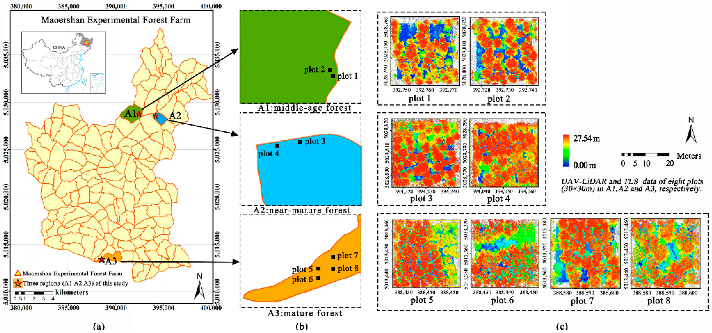
2.1. Study Area and Sampling

The study area is located in the Maoershan Experimental Forest Farm, Shangzhi City, Heilongjiang Province, China, from 127°29′E to 127°44′E and 45°14′N to 45°29′N (Figure 1a). The slope ranges from 5° to 25°, and the terrain is mountainous, rising from south to north with an average elevation of about 300 m. This region has a temperate continental monsoon climate. Maoershan is a typical natural secondary forest in northeastern China surrounded by various broadleaved trees, such as white birch (Betula platyphylla Suk.), Mongolia oak (Quercus mongolica Fisch. ex Ledeb.), and Korean aspen (Populus davidiana), and a few coniferous trees, such as Changbai larch (Larix olgensis Henry), Mongolian pine (Pinus sylvestris var. mongolica Litv.), and Korean pine (Pinus koraiensis Sieb. et Zucc.).

The eight sample plots of 0.09 ha (30 × 30 m) were selected from three larch plantations regions according to different site conditions and forest stages (A1: middle-age forest; A2: near-mature forest; A3: mature forest) (Figure 1b). The normalized UAV-LiDAR and TLS point data of the eight sample plots were shown in Figure 1c.

2.2. Data and Preprocessing

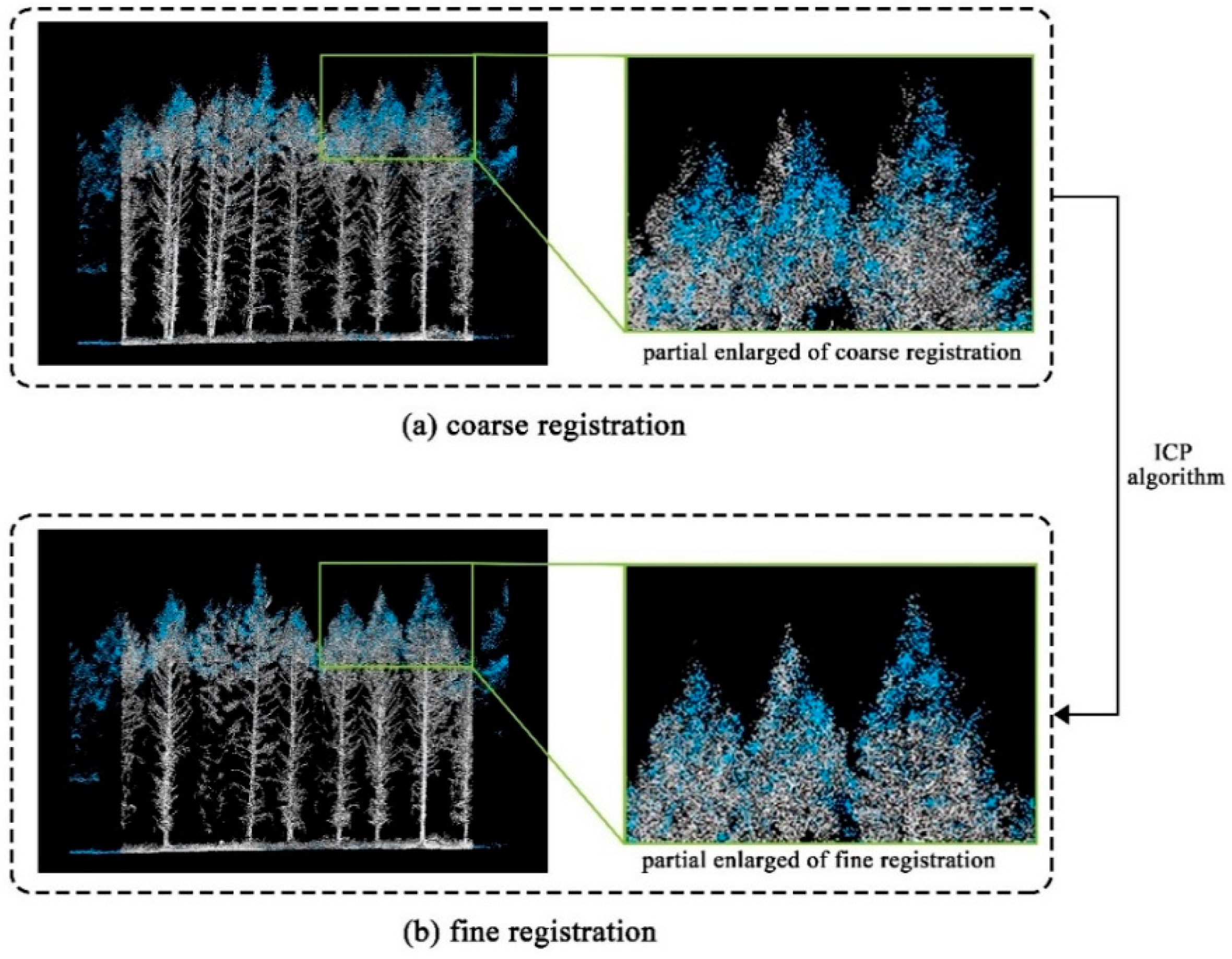
2.2.1. LiDAR Data and Preprocessing

UAV-LiDAR data used in this study were acquired in August 2020. The UAV-borne LiDAR equipment was RIEGL mini VUX-1UAV-LiDAR scanner (Horn, Austria, https://www.riegl.com/products/unmanned-scanning/riegl-minivux-1uav, accessed on 14 June 2022) carried by a Feima D200 UAV platform (Shenzhen, China, https://www.feimarobotics.com/en/productDetailD200, accessed on 14 June 2022). All the flights were designed as crossed transects with 50% swath overlaps at 80 m altitude and 5.0 m/s speed. Raw UAV-LiDAR data were denoised and then classified into non-ground points and ground points using the improved progressive triangulated irregular network (TIN) densification (IPTD) filtering algorithm [59] in the Green Valley International^® LiDAR360 software (v 5.0) (Berkeley, CA, USA, https://greenvalleyintl.com/software, accessed on 14 June 2022).

TLS data of eight sample plots were acquired in September 2020 using a Riegl VZ-400i (RIEGL, Horn, Austria, https://www.riegl.com, accessed on 14 June 2022). In order to ensure the spatial coverage of each station, 11 to 13 scanning stations were set up for each plot. TLS data were registered to WGS 84-UTM zone 52N projection coordinate system using the real-time kinematic (RTK) global positioning system receiver. The point cloud data of multiple stations were co-registered and integrated into plot-level point cloud data using the Riegl RiSCAN PRO software package (v 2.7.1). Due to a large amount of TLS point cloud data, the point cloud was thinned by an octree-based algorithm [60] in terms of speed and computational complexity, following noise elimination. Subsequently, the thinned point clouds were filtered into ground and non-ground points using IPTD filtering algorithm in LiDAR360 software. The main parameters of the two LiDAR data used in this study are shown in the

Table A1. The main parameters of the two LiDAR data used in this study.

Parameters	UAV-LiDAR	TLS
Sensor	RIEGL mini VUX-1UAV	RIEGL VZ-400i
Wavelength (nm)	905	1550
Point frequency (Hz)	100 k	1200 k
Ranging accuracy (mm)	±10	±5
Scan frequency (Hz)	10–100	100–1200 k
Field of view (°)	360	360 × 100
Average point density (pts/m2)	111	275,606

of Appendix A.

2.2.2. Field Inventory Data

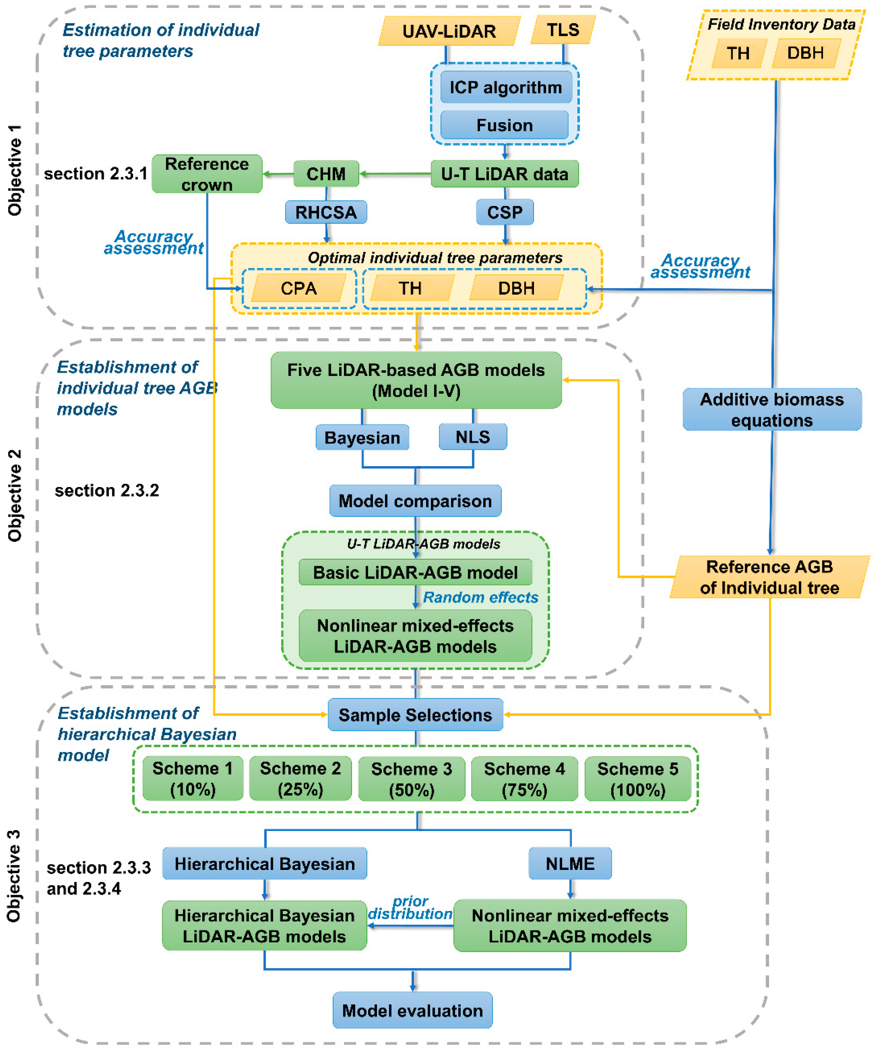
In this study, all the trees with a DBH equal or greater than 5 cm in eight plots were recorded. In total, four individual tree parameters of 370 Changbai larch trees in eight plots were measured and recorded, including DBH (cm), tree height (TH) (m), tree species, and location. There were 123, 98, and 149 trees in middle-age, near-mature, and mature forest, respectively. DBH was measured using a perimeter ruler; tree height was measured using the Vertex IV ultrasound instrument system, and the location of each tree was recorded using RTK with positional error estimated to be within 5 cm. The descriptive statistics of the main variables are presented in

Table 1. Descriptive statistics of field measurements (i.e., DBH and TH) and reference AGB of individual tree used in this study.

Regions	Forest Stages	Planting Years	Plot Number	N	DBH (cm)		TH (m)		Reference AGB (kg)
					Mean	Std	Mean	Std	Mean	Std
A1	Middle-age forest	1990	1	61	19.53	5.16	17.78	2.65	152.81	93.41
		1990	2	62	19.98	5.28	17.62	2.95	157.56	89.94
A2	Near-mature forest	1985	3	51	23.67	7.03	22.63	2.48	337.45	144.17
		1985	4	47	28.73	6.29	23.36	2.04	401.08	171.83
A3	Mature forest	1978	5	64	22.86	5.43	21.12	2.87	243.75	114.67
		1978	6	32	28.61	5.14	24.41	1.30	410.56	141.23
		1978	7	28	30.25	3.66	24.83	1.01	457.95	114.41
		1978	8	25	32.97	6.99	24.42	3.17	546.15	185.02

.

2.3. Methods

In this study, the preprocessed UAV-LiDAR and TLS data were registered and fused to create the U-T LiDAR data for comprehensively describing individual tree structure. Firstly, based on the U-T LiDAR data, two algorithms (CSP and RHCSA) were used to delineate individual trees and obtain the optimal LiDAR-derived individual tree parameters (i.e., DBH, TH, and CPA) based on field inventory data (objective 1). Secondly, five widely used AGB model forms (model I-V) were selected and compared by NLS and Bayesian approach based on the reference AGB of individual tree, and the corresponding mixed-effects LiDAR-AGB model was developed with random effects for different regions to further improve the model fitting (objective 2). Then, the hierarchical Bayesian and NLME methods were compared to estimate individual tree AGB with five sample sizes (i.e., 10%, 25%, 50%, 75%, and 100%) in order to explore the appropriate sample size that could balance between the estimation accuracy and cost (objective 3). A flowchart of this study is depicted in Figure 2. Section 2.3.1, Section 2.3.2, Section 2.3.3, and Section 2.3.4 explained the procedure for objectives 1, 2, and 3, respectively.

2.3.1. Estimation of Individual Tree Parameters

The UAV-LiDAR and TLS data for each sample plot were coarsely registered based on the projected coordinate system. Then, the iterative closest point (ICP) algorithm, a point-based matching method based on minimizing the cumulative distance between two LiDAR data [26,61], was used to conduct a fine co-registration of the two LiDAR data in this study. In this study, UAV-LiDAR was set as the reference point cloud for registering TLS data. After the coarse and fine registration (Figure 3), the UAV-LiDAR and TLS data for each plot were fused in LiDAR360 software.

This study used two segmentation algorithms (CSP and RHCSA) to segment individual trees based on the normalized fused LiDAR (U-T LiDAR) data. The CSP algorithm proposed by Tao et al. [34] finds seed points of individual trees by recognizing tree bases and then labels other points by finding the shortest path to the seed points, which has been directly applied to LiDAR point data [23,62]. In addition, the RHCSA algorithm was applied to segment individual trees based on the canopy height model (CHM) derived from the U-T LiDAR data. RHCSA is a one-step individual tree crown delineation (ITCD) algorithm, which segments individual trees with a few user-defined parameters [15]. The appropriate cell size of CHM could reduce the errors of segmentation and ensure that sufficient detail is maintained in the height model [63]. This study employed kriging interpolation with a pixel size of 0.25 m through trial and error. The smoothed CHM eliminated the majority of noise and empty sinks, allowing for an accurate interpretation of tree crowns [64].

The local maxima of height within each tree crown and the projection area of delineated crowns from the segmentation algorithms were defined as TH and CPA, respectively. The DBH of individual trees was estimated using a nonlinear least-squares circle fitting algorithm [65,66]. The position of the treetop was considered to be the tree location. All of the individual tree parameters (i.e., tree location, DBH, TH, and CPA) were estimated using LiDAR360 5.0 and ArcGIS 10.4 (ESRI, Redlands, CA, USA) software.

The accuracy assessment of two segmentation algorithms was evaluated based on the three indices, including recall (r), precision (p), and F-score (F) [30]. The three indices were calculated using the following equations:

$$r=\frac{TP}{TP+FN}$$

(1)

$$p=\frac{TP}{TP+FP}$$

(2)

$$F=2\times \frac{r\times p}{r+p}$$

(3)

where $TP$ ($\mathrm{true} \mathrm{positive}$) denotes the number of trees correctly detected, that is, 1:1 matched trees; $FN$ (false negative) denotes the number of trees that were not detected; and $FP$ (false positive) denotes the number of trees falsely detected. $r$ indicates the tree segmentation completeness, $p$ indicates the correctness of the detected trees, and $F$ is the overall accuracy considering both commission and omission errors. In this study, 1:1 matched trees were defined as the trees located within 3 m of the reference tree position and had the minimum differences of DBH from references within the 20% of the average plot value [67].

Based on 1:1 matched trees, the accuracy of DBH and TH were evaluated using the field measurements. Since two-dimensional parameter CPA is difficult to measure in the field and no allometric equation is available to estimate CPA for Changbai larch, the accuracy of CPA was evaluated using the CHM-based manual delineation. The accuracies of estimated individual tree parameters were assessed by the coefficient of determination (R²) of the regression between estimated and measured parameters, root-mean-square error (RMSE), and relative root-mean-square error (rRMSE) of estimated parameters as follows.

$$R^2=\frac{{{\displaystyle \sum }}_{i=1}^n\left(y_i-\overline{y_i}\right)\left(\widehat{y_i}-\overline{\widehat{y_i}}\right)}{\sqrt{{{\displaystyle \sum }}_{i=1}^n{\left(y_i-\overline{y_i}\right)}^2}\sqrt{{{\displaystyle \sum }}_{i=1}^n{\left(\widehat{y_i}-\overline{\widehat{y_i}}\right)}^2}}$$

(4)

$$RMSE=\sqrt{\frac{1}{n}{\displaystyle \sum }_{i=1}^n{\left(y_i-\widehat{y_i}\right)}^2}$$

(5)

$$rRMSE=\frac{RMSE}{\overline{y_i}}\times 100\%$$

(6)

where $y_i$ is the reference parameters of individual trees, $\widehat{y_i}$ is the estimated parameters, $\overline{y_i}$ is the mean value of the reference parameters, $\overline{\widehat{y_i}}$ is the mean value of estimated parameters, and n is the number of samples.

2.3.2. Establishment of Individual-Tree AGB Model Based on U-T LiDAR

Five common candidate models established with the three optimal individual tree parameters (DBH, TH, and CPA) were applied as the basic U-T LiDAR-AGB models (baseline) in this study [21,68]. The five AGB models are listed as follows.

$$\mathrm{Model} \mathrm{I}: AGB=a_1·DB{H}^{a_2}+\epsilon$$

(7)

$$\mathrm{Mode} \mathrm{II}: AGB=a_1·DB{H}^{a_2}·T{H}^{a_3}+\epsilon$$

(8)

$$\mathrm{Model} \mathrm{III}: AGB=a_1·DB{H}^{a_2}·CP{A}^{a_3}+\epsilon$$

(9)

$$\mathrm{Model} \mathrm{IV}: AGB=a_1·T{H}^{a_2}·CP{A}^{a_3}+\epsilon$$

(10)

$$\mathrm{Model} \mathrm{V}: AGB=a_1·DB{H}^{a_2}·T{H}^{a_3}·CP{A}^{a_4}+\epsilon$$

(11)

where DBH denotes the diameter at breast height (cm), TH is tree height (m), CPA presents tree crown projection (m²), AGB is reference AGB, and $\epsilon$ is an error term. The reference AGB of individual tree in this study was calculated using the additive biomass equations of larch plantations proposed by Dong et al. [69], shown in

Table A2. The structure of additive biomass equations with different components (stem, branch, foliage) and AGB for Changbai larch in northeastern China, sourced from Dong et al. ($W_s$, stem biomass; $W_b$, branch biomass; $W_f$, foliage biomass; $W_a$, AGB).

Component	Models
Stem	$\ln W_s=-4.5363+1.7008·\ln DBH+1.4804·\ln TH$
Branch	$\ln W_b=-3.3632+2.6728·\ln DBH-0.7052·\ln TH$
Foliage	$\ln W_f=-2.2879+1.3369·\ln DBH-0.0922·\ln TH$
AGB	$\ln W_a=\ln (W_s+W_b+W_f)$

of Appendix A.

Due to the stratified structure of the data (i.e., sample trees in three regions of different forest stages, including A1: middle-age forest, A2: near-mature forest, and A3: mature forest), the NLME approach [70] was used for the basic LiDAR-AGB model in this study. All parameter combinations were simulated as mixed parameters, with Akaike’s information criterion (AIC), Bayesian information criterion (BIC), and log-likelihood ($LL$) serving as the primary evaluation criteria for the fitting performance. The specific mixed-effects U-T LiDAR-AGB model form is established based on the basic U-T LiDAR model, with the mixed-effects model parameters estimated using the maximum likelihood method (ML) with the nlme function of the nlme library in R software 4.0.3 (New York, NY, USA, https://mran.microsoft.com/, accessed on 14 June 2022).

2.3.3. Establishment of Hierarchical Bayesian Model

Based on the advantage of the Bayesian method for small sample estimation and the stratified structure of the data, hierarchical Bayesian models were established. However, to ensure an adequate sample size, this study selected five sample sizes (samples 1–5) using stratified random sampling with a proportional allocation. Sample 1–5 was stratified randomly selected using a proportion of 10%, 25%, 50%, 75%, and 100% in each forest stage (i.e., A1: middle-age forest, A2: near-mature forest, and A3: mature forest), respectively.

The Bayesian approach is a statistical framework that combines new evidence (data) with prior distributions of parameter values to derive new probability for various parameter values [47,71]. It is also suitable for multilevel analysis [72], where the regions (i.e., A1, A2, and A3) are considered as random variables. The AGB data can be used to estimate parameter $\theta$ for each region. Let $y=\left(y_{1j}, \dots , y_{ij}\right)$ represents the AGB data vector, $y_{ij}$ is the AGB of the $i$th tree in the region j; let $\theta =\left({\theta }_1, {\theta }_2, {\theta }_3 \dots \right)$ represent the vector of parameters to be estimated. Then $\pi (\theta |\lambda )$ is determined, where $\lambda$ is a hyperparameter vector [73]. The inference parameter $\theta$ is based on its posterior distribution:

$$p\left(\theta |y,\lambda \right)=\frac{p(y,\theta |\lambda )}{{{\displaystyle \int }}^{ }p(y,\theta |\lambda )d\theta }=\frac{f(y|\theta )·\pi (\theta |\lambda )}{{{\displaystyle \int }}^{ }f(y|\theta )·\pi (\theta |\lambda )d\theta }$$

(12)

The prior distribution of $\pi (\theta |\lambda )$ in this study is obtained from the parameters estimated by NLME [73]. The posterior distribution is used for Bayesian statistical inference, assuming $\theta$ is known, $f(y|\theta )$ provides the distribution of $y$, which is considered a likelihood function when viewed as a function of the parameters.

For the Bayesian estimation, a burn-in period of 30,000 steps and 330,000 iterations were used to estimate parameters. The thinning parameter was set to 3 to reduce the correlation between neighboring iterations. In this study, Bayesian models were developed using the MCMC procedure in SAS 9.4, and the average running time for each model was approximately three minutes.

2.3.4. Model Evaluation

The best AGB model was selected by both the classical method and Bayesian method from the smallest AIC, BIC, and deviance information criterion (DIC) when pooling the data. Moreover, the stationarity test of Heidelberger–Welch Diagnostics [74,75] was conducted to test whether the model converged in this study. The DIC is calculated by:

$$DIC=\overline{D}+p_D$$

(13)

where $\overline{D}$ is the posterior mean of the deviance (−2 $\times$ Log likelihood of the given data and parameters), and $p_D$ is the model complexity, which is summarized by the effective number of parameters.

The Fit Index (FI) [76,77] and the root mean square error (RMSE) were applied to compare the Bayesian method with the classical method on different sample sizes. Larger FI and smaller RMSE values indicate a better model fitting. The FI are calculated by:

$$FI=1-\frac{{{\displaystyle \sum }}_{i=1}^n{\left(y_i-\widehat{y_i}\right)}^2}{{{\displaystyle \sum }}_{i=1}^n{\left(y_i-\overline{y_i}\right)}^2}$$

(14)

where $y_i$, $\widehat{y_i}$ and $\overline{y_i}$ represent the observed, estimated, and mean values of AGB, respectively.

3. Results

3.1. Estimation of Individual Tree Parameters

The average F (F-score) value of eight sample plots for the two segmentation algorithms was above 0.90 (

Table 2. The plot-level accuracy assessment for the two segmentation algorithms based on U-T LiDAR data.

Algorithms	r *	p *	F *	TP (1:1 Matched Trees)	FP	FN
CSP	0.90	0.94	0.92	337	20	33
RHCSA	0.88	0.93	0.90	327	24	43

Note: * represented the average r, p, and F value of eight sample plots; TP, FP, and FN were the total value of true positive (1:1 matched trees), false positive, and false negative for eight sample plots, respectively. CSP: comparative shortest-path algorithm, RHCSA: region hierarchical cross-sectional analysis algorithm.

). The CPS algorithm was slightly better than the RHCSA algorithm for individual tree segmentation (0.92 vs. 0.90). A total of 337 sample trees were correctly segmented and matched using the CSP algorithm from 370 reference trees. The RHCSA algorithm, based on CHM for individual tree segmentation, had weaknesses in detecting small trees: the number of correctly detected trees (TP) of RHCSA was slightly fewer than the CSP algorithm (327 vs. 337 out of 370).

Table 3. The accuracy assessment of individual tree parameters for the two segmentation algorithms.

Algorithms	N	Parameters	R2	RMSE	rRMSE (%)
CSP	337	DBH	0.983	1.017	4.9
		TH	0.923	1.494	8.3
		CPA	0.527	29.258	607.3
RHCSA	327	DBH	0.990	1.024	4.8
		TH	0.934	1.247	7.3
		CPA	0.905	3.874	43.7

Note: N is the number of 1:1 matched trees, DBH presented diameter at breast height (cm), TH presented tree height (m), CPA presented tree crown projection (m²).

presents that the R² of individual tree parameters are all greater than 0.9, except the CPA estimated by CSP. It is because that lots of points from shrubs near the ground were misclassified as tree points by the CSP algorithm, and the CSP algorithm calculated CPA based on the average crown diameter estimated by the tree points, therefore resulting in larger estimated canopy diameters and CPA. The RMSE and rRMSE values of TH and CPA estimated by RHCSA were lower than those estimated by CSP. In addition, the accuracies of DBH estimated by CSP and RHCSA were very similar (R²: 0.983 vs. 0.990, RMSE: 1.017 vs. 1.024; rRMSE: 4.9 vs. 4.8). To ensure the accuracy of individual tree AGB estimates, we applied the individual tree parameters of 327 sample trees based on the RHCSA algorithm as the predictor variables for the subsequent individual tree AGB estimation.

3.2. Establishment of Individual-Tree AGB Model Based on U-T LiDAR

Table 4. The fitness statistics of the five widely used AGB models using classical and Bayesian approaches.

Model No.	Model Forms	Classical Approach		Bayesian Approach
		AIC	BIC	DIC	Stationarity Test
I	$AGB=a_{1}DB{H}^{a_2}+\epsilon$	3308.285	3319.655	3297.941	Passed
II	$AGB=a_{1}DB{H}^{a_2}T{H}^{a_3}+\epsilon$	3044.183	3059.343	3036.874	Passed
III	$AGB=a_{1}DB{H}^{a_2}CP{A}^{a_3}+\epsilon$	3309.353	3324.513	3307.981	Passed
IV	$AGB=a_{1}T{H}^{a_2}CP{A}^{a_3}+\epsilon$	3743.494	3758.654	-	Failed
V	$AGB=a_{1}DB{H}^{a_2}T{H}^{a_3}CP{A}^{a_4}+\epsilon$	3039.067	3058.017	3032.190	Passed

Note: DBH presented diameter at breast height, TH presented tree height, CPA presented crown projection area, ε presented error term.

shows the fitness statistics of the five widely used AGB models using both classical and Bayesian approaches in this study. Model V showed the best evaluation statistics with the smallest AIC (3039.067), BIC (3058.017), and DIC (3032.190) values among the five models, while Model IV had the worst model performance and even failed the Heidelberger–Welch Diagnostics test for the stationarity.

Model V (Equation (11)) with three predictor variables (i.e., DBH, TH, and CPA) was selected as the basic U-T LiDAR-AGB model due to the best model performance (Table 4). According to $AIC$, $BIC$ and $LL$ values of all combinations of parameter and random effect (i.e., A1, A2, A3) (see the

Table A3. The model evaluation statistics of all parameter combinations.

Parameter Combinations	AIC	BIC	LL
$a_1$	3032.088	3054.828	−1510.044
$a_2$	3031.211	3053.950	−1509.606
$a_3$	3031.709	3054.449	−1509.854
$a_4$	3029.853	3052.593	−1508.927
$a_1$ $a_2$	3035.211	3065.531	−1509.606
$a_1$ $a_3$	3036.087	3066.406	−1510.043
$a_1$ $a_4$	3032.164	3062.483	−1508.082
$a_2$ $a_3$	3033.269	3063.588	−1508.634
$a_2$ $a_4$	3031.936	3062.256	−1507.968
$a_3$ $a_4$	3031.729	3062.048	−1507.864
$a_1$ $a_2$ $a_3$	-	-	-
$a_1$ $a_2$ $a_4$	3038.164	3079.854	−1508.082
$a_2$ $a_3$ $a_4$	-	-	-
$a_1$ $a_3$ $a_4$	-	-	-
$a_1$ $a_2$ $a_3$ $a_4$	-	-	-

Note: - means model failed to converge.

of Appendix A), mixed-effects U-T LiDAR-AGB models were established by adding a random effect parameter to $a_4$ based on model V as Equation (15). The model evaluation statistics of all parameter combinations are shown in Table A1.

$$AG{B}_{ij}=a_{1}DB{H}_{ij}^{a_2}T{H}_{ij}^{a_3}CP{A}_{ij}^{\left(a_4+a_i\right)}+{\epsilon }_{ij}$$

(15)

where $a_1$–$a_4$ are the parameters of the model, $a_i$ is the random-effect parameter of the ith region; $AG{B}_{ij}$, $DB{H}_{ij}$, $T{H}_{ij}$, $CP{A}_{ij}$ and ${\epsilon }_{ij}$ are the individual tree AGB (kg), DBH (cm), TH (m), CPA (m²), and random error term of tree $j$ from the ith region, respectively.

Table 5. Parameter estimates and standard deviations (values in brackets) and fitting goodness of the basic U-T LiDAR-AGB model (model V) using NLS and NLME methods.

Types	Parameters	NLS	NLME
Fixed effects	$a_1$	0.024 (0.004)	0.026 (0.004)
	$a_2$	1.795 (0.036)	1.807 (0.035)
	$a_3$	1.128 (0.057)	1.102 (0.060)
	$a_4$	0.032 (0.012)	0.023 (0.013)
Random effect	$StdDev\left(a_i\right)$	-	0.0053
Fitting	$FI$	0.979	0.981
	$RMSE\left(\mathrm{kg}\right)$	24.893	24.183
	$AIC$	3039.067	3029.853
	$BIC$	3058.017	3052.593

Note: NLS: nonlinear least squares; NLME: nonlinear mixed effect model.

shows the fitting goodness of the basic U-T LiDAR-AGB model (model V) using nonlinear least squares (NLS) and NLME methods. All model parameters were significant, and the NLME method fitting substantially improved. The FI of the mixed-effects model was higher than that of the basic model (0.981 vs. 0.979), and RMSE, AIC, and BIC values decreased. However, there was no significant difference in the standard deviations of the parameters between the two methods. Both models showed an ideal fitting effect.

3.3. Establishment of Hierarchical Bayesian Models with Different Sample Sizes

According to stratified random sampling with proportional allocation, five sample sizes decreased from 327 (100%) to 34 (10%) trees were applied for hierarchical Bayesian modeling in this study (see the

Table A4. The basic statistics of individual tree parameters (DBH, TH, CPA and AGB) with different sample sizes.

Sample Sizes (Proportions)	Variables	Mean	Standard Deviation	Minimum	Maximum
327 (100%)	$DBH$ (cm)	24.69	6.81	10.00	42.30
	$TH$ (m)	21.86	3.09	11.27	27.54
	$CPA$ (m2)	14.81	8.67	0.94	58.44
	AGB (kg)	301.03	174.91	24.11	951.38
246 (75%)	$DBH$ (cm)	24.84	6.78	10.20	42.30
	$TH$ (m)	21.96	2.96	13.29	27.54
	$CPA$ (m2)	15.24	9.10	0.94	58.44
	AGB (kg)	305.13	177.56	31.56	951.38
164 (50%)	$DBH$ (cm)	24.34	6.77	10.00	42.30
	$TH$ (m)	21.87	3.19	11.64	27.54
	$CPA$ (m2)	14.82	7.79	0.94	37.00
	AGB (kg)	293.77	177.97	38.08	951.38
82 (25%)	$DBH$ (cm)	25.00	7.79	10.10	42.30
	$TH$ (m)	21.97	3.15	11.27	27.54
	$CPA$ (m2)	15.44	9.63	1.06	53.00
	AGB (kg)	322.26	208.51	24.11	951.38
34 (10%)	$DBH$ (cm)	24.27	7.17	10.70	40.20
	$TH$ (m)	21.69	2.73	16.53	26.30
	$CPA$ (m2)	15.73	11.29	1.06	53.00
	AGB (kg)	287.51	188.48	41.47	833.04

Note: DBH presented LiDAR-derived diameter at breast height, TH presented LiDAR-derived tree height, CPA presented LiDAR-derived crown projection area.

of Appendix A). The basic statistics of individual tree parameters (DBH, TH, CPA, and AGB) for each sample size are summarized in Table A4.

The hierarchical Bayesian models were compared to the corresponding NLME models using different sample sizes. The prior parameter distribution of Bayesian estimation was obtained from the parameters of NLME estimation. The posterior probability distributions of the parameters estimated by the Bayesian theory for U-T LiDAR-AGB models are summarized in

Table 6. Parameter estimates with standard errors/deviations (values in parentheses) and the accuracy of the U-T LiDAR-AGB model using five sample sizes.

Methods	Parameters	Sample Sizes (Proportions)
		34 (10%)	82 (25%)	164 (50%)	246 (75%)	327 (100%)
Hierarchical Bayesian	$a_1$	0.014 (0.004)	0.028 (0.001)	0.032 (0.005)	0.027 (0.003)	0.025 (0.002)
	$a_2$	2.029 (0.051)	1.759 (0.002)	1.790 (0.038)	1.807 (0.012)	1.801 (0.030)
	$a_3$	1.086 (0.112)	1.087 (0.102)	1.105 (0.053)	1.084 (0.041)	1.107 (0.036)
	$a_4$	0.009 (0.020)	0.079 (0.001)	0.033 (0.016)	0.029 (0.010)	0.031 (0.011)
	FI	0.987	0.984	0.983	0.981	0.980
	RMSE (kg)	14.866	22.317	22.372	24.491	24.863
NLME	$a_1$	0.012 (0.006)	0.025 (0.007)	0.030 (0.006)	0.027 (0.005)	0.026 (0.004)
	$a_2$	2.029 (0.141)	1.756 (0.069)	1.807 (0.058)	1.808 (0.041)	1.807 (0.035)
	$a_3$	1.124 (0.185)	1.124 (0.107)	1.051 (0.080)	1.083 (0.069)	1.102 (0.060)
	$a_4$	0.009 (0.041)	0.078 (0.023)	0.025 (0.020)	0.023 (0.015)	0.023 (0.013)
	FI	0.987	0.981	0.981	0.980	0.981
	RMSE (kg)	21.662	23.856	23.542	25.006	24.146

Note: The values in parentheses presented the standard errors or standard deviation of the parameters estimates obtained by the hierarchical Bayesian approach or NLME approach, respectively.

. Although the parameter estimates using the two approaches were very similar, the standard errors of the estimates obtained by the hierarchical Bayesian method in all sample sizes were smaller than those obtained by the classical NLME method. This implies that the Bayesian method provided more stable estimates than the classical method. Figure 4 compares the parameters estimated by the hierarchical Bayesian and NLME methods with the 95% confidence intervals based on the five sample sizes. The hierarchical Bayesian method produced estimates with a narrower 95% confidence interval than the NLME method for all sample sizes. The parameter estimates were more stable for smaller sample sizes, especially the sample size of 82, than for larger sample sizes (e.g., 327) when the hierarchical Bayesian method was applied.

Table 6 also confirms that the difference between FI and RMSE between the two methodologies became obvious with decreasing sample sizes. For example, when pooling the data (n = 327), the FI and RMSE of the Bayesian method were very similar to that of the classical method (0.980 vs. 0.981; 24.863 vs. 24.164). When the sample size was reduced to 34, however, the performance of the Bayesian method was much better than that of the classical method: the RMSE decreased by 31.4%.

4. Discussion

Although it is a widely used method to estimate individual tree AGB using an allometric equation based on field inventory data (e.g., DBH, TH), its efficiency and accuracy are still unsatisfactory, particularly for large-scale forest inventory [78]. This study provided a potential solution for establishing an efficient model using combined UAV and terrestrial LiDAR data with an appropriate sample size based on the hierarchical Bayesian method.

4.1. Individual Tree Parameters Estimation Using U-T LiDAR Data

The near-surface LiDAR is a non-destructive technology widely used in forest inventory and AGB estimation in recent years [19,21,51]. However, single platform/single-scan LiDAR data have limitations; the U-T LiDAR data combines the rich point cloud beneath the canopy obtained from TLS with middle and upper canopy information from UAV-LiDAR. U-T LiDAR data could accurately capture tree trunk parameters (e.g., DBH), TH, and crown structural parameters (e.g., CPA) with a broader viewing angle than field measurements, resulting in a satisfactory AGB estimation accuracy for individual trees.

The accuracy of individual tree segmentation may significantly impact the acquisition of individual tree parameters [26]. Based on the U-T LiDAR data, CHM-based and point cloud-based segmentation algorithms (RHCSA and CSP) were used to segment individual trees in this study. The average plot-level F-scores (0.90 and 0.92 using RHCSA and CSP, respectively) were similar but slightly higher than the other studies. For example, Li et al. [30] reported an average F-score of 0.90 for mixed conifer forests based on the airborne LiDAR data using the PCS algorithm. Tao et al. [34] reported an average F-score of 0.87 for three forest types (i.e., conifers, broadleaf, and mixed) using the CSP algorithm based on terrestrial and mobile LiDAR data. Similar to the previous studies, compared to the PCS algorithm, the CHM-based methods (RHCSA in this study) had weaknesses in detecting small trees, especially for high canopy closure forests [79]. A total of 91.1% and 88.4% of sample trees were correctly segmented and matched by the CSP and the RHCSA algorithm. However, the CPA estimated using the CSP algorithm had much lower accuracy than that of the RHCSA algorithm. This could be because the CSP is a bottom-up algorithm; points from shrubs near the ground could be misclassified as sample tree points, resulting in trees with larger estimated canopy diameters. Furthermore, the CSP algorithm computed the circle area as CPA using the average crown diameter derived from the point cloud. In contrast, the RHCSA algorithm delineated entire tree crowns using CHM from a vertical perspective, making it easier to visualize and estimate CPA than CSP. Due to the similar reasons, the tree height estimated using CSP had a slightly lower accuracy (R² = 0.923, RMSE = 1.494 m, rRMSE = 8.3%) than that of RHCSA (R² = 0.934, RMSE = 1.247 m, rRMSE = 7.3%). Little difference was observed in the accuracy of DBH extracted by the two algorithms. The results demonstrated the potential of applying multi-platform LiDAR data to derive individual tree parameters for individual tree AGB estimation in lieu of field measurements to some extent.

4.2. The Hierarchical Bayesian Method in AGB Estimation

With the widespread use of the MCMC algorithm and the advancement of computing technology, Bayesian-based applications in forestry have become increasingly popular in recent years [41,46,55]. Although the Bayesian and classical methods in this study showed a similar trend in the basic LiDAR-AGB model selection (Model V was the best, followed by Model II, and Model IV was the worst), the Bayesian method is more rigorous (Table 4). The findings were consistent with that of Fu et al. [21]. However, Wang et al. [51] selected a basic LiDAR-AGB model with DBH and CPA as predictors (model III in this study) due to the LiDAR data obtained from a different platform (i.e., airborne) and the method of estimating individual tree parameters.

The mixed-effects and hierarchical Bayesian models are versatile and applicable for constructing regional biomass models [1]. Based on the stratified data structure, the NLME method of the frequentist paradigm and the hierarchical Bayesian method of the Bayesian paradigm were implemented and compared using regions as the random effect. The hierarchical Bayesian model assumes that parameters are defined from prior distributions. In previous studies [4,80], non-informative priors with enormous or infinite variance were commonly used, and the parameter estimation was always identical to the frequentist paradigm. In this study, the prior distribution of the hierarchical Bayesian method was obtained from the parameters estimated by the classical statistical approach (NLME) according to Zhang et al. [81] and Wang et al. [51]. Alternatively, parameter prior information of some studies was derived from external knowledge (reported parameters from the literature) (e.g., [1]). The impact of prior information on model fitting should be investigated in future research. In addition, the parameters estimated by the hierarchical Bayesian method were more stable than the classical method, with smaller standard errors/deviations and narrower 95% intervals (Table 6 and Figure 4). That is consistent with the results of Wang et al. [51]. Based on the evaluation statistics of FI and RMSE, with the decreasing sample size, the Bayesian method showed obvious advantages (Table 6). For the sample size of 34, the RMSE was a 31.4% reduction compared to the classical method. This is in agreement with the findings of Wang and Zapata-Cuartas [44,51].

This study found that the LiDAR-AGB model with the U-T LiDAR-derived individual tree parameters as predictor variables could achieve better prediction results using the hierarchical Bayesian method, particularly when the sample size was small (34 trees in this study). The parameter estimations were more stable, and the model fitting was better than the classical method. Similarly, Wang et al. [51] estimated the individual tree AGB based on 39 sample trees of Qinghai spruce (Picea crassifolia Kom) using the layered Bayesian method, achieving a result of R² = 0.8611. Thus, there is great potential for using the hierarchical Bayesian method with small sample sizes (less than 50) to estimate the individual tree AGB.

4.3. Limitations

There are still limitations that need to be discussed. First, it should be recognized that field-estimated AGB is commonly referred to as reference data in remote sensing studies (e.g., [51,55]) in order to avoid destructive biomass sampling in the field and improve efficiency. However, the accuracy of field estimates is unknown, indicating that the ‘ground truth’ of the individual tree-level AGB may have uncertainty [82]. Although both errors due to tree measurement and the choice of an allometric model are sources of AGB estimation uncertainty, several pieces of research have revealed that the most significant sources of error are currently related to the choice of an allometric model [83]. More work should be devoted to considering these uncertainties derived from remotely sensed data. Second, the efficacy of TLS data in forest stands with dense canopies is inferior to that of BLS due to the inconvenient transport of TLS equipment to sample plots or the difficulty in changing stations in dense forests. In this study, for instance, about ten scanning stations were set up for each sample plot (30 × 30 m), requiring two personnel to operate for 2–3 h to complete the TLS data collection of each plot, with an average stand density of 810 trees/ha. However, BLS may have relatively low accuracy for individual tree parameters due to the lack of points for the middle and upper parts of trees [27]. In practice, the number of TLS scanning stations should be adjusted according to study objectives and stand density to balance efficiency and accuracy. Compared to conventional measurements, combining ULS and TLS data provides a comprehensive, efficient, and cost-effective method for obtaining individual tree properties. Moreover, although the hierarchical Bayesian approach has improved the stability of model parameters compared with the classic NLME method, it does not show significant advantages in model parameter estimation, especially for large sample sizes. Therefore, the hierarchical Bayesian method should be applied according to the study objective and sample size and is still worth further exploration in forestry.

5. Conclusions

This study investigated the applicability of fusing UAV and terrestrial LiDAR data and the feasibility of hierarchical Bayesian for non-destructive individual tree AGB estimation of Changbai larch (Larix olgensis Henry) in northeastern China. When taking the full advantages of UAV and terrestrial platforms, the U-T LiDAR data estimated the individual tree parameters (i.e., DBH, TH, and CPA) of Changbai larch with high accuracies (all R² > 0.9) using RHCSA segmentation algorithm. Considering regions as random variables, the nonlinear mixed-effects U-T LiDAR-AGB model with three predictor variables (i.e., DBH, TH, and CPA) performed better than its corresponding nonlinear model. In addition, the hierarchical Bayesian method provided better performances and more stable parameter estimates than the classical method, especially for small sample sizes (e.g., <50). This study implied that the fused multi-platform LiDAR data combined with the hierarchical Bayesian method have the potential to improve the accuracy of individual tree AGB estimation, which provides a non-destructive approach for individual tree AGB modeling with a small sample size. This methodology of this study (i.e., multi-platform LiDAR data and the hierarchical Bayesian method) could provide a scientific basis for non-destructive individual tree AGB modeling with a small sample size and high accuracy in the future.

References

1. Chen, D.; Huang, X.; Zhang, S.; Sun, X. Biomass Modeling of Larch (Larix spp.) Plantations in China Based on the Mixed Model, Dummy Variable Model, and Bayesian Hierarchical Model. Forests 2017, 8, 268. [Google Scholar] [CrossRef]
2. Gleason, C.J.; Im, J. A Review of Remote Sensing of Forest Biomass and Biofuel: Options for Small-Area Applications. GISci. Remote Sens. 2011, 48, 141–170. [Google Scholar] [CrossRef]
3. Pan, Y.; Birdsey, R.A.; Fang, J.; Houghton, R.; Kauppi, P.E.; Kurz, W.A.; Phillips, O.L.; Shvidenko, A.; Lewis, S.L.; Canadell, J.G.; et al. A Large and Persistent Carbon Sink in the World’s Forests. Science 2011, 333, 988–993. [Google Scholar] [CrossRef] [PubMed]
4. Zhang, X.; Duan, A.; Zhang, J.; Muldoon, M.R. Tree biomass estimation of Chinese fir (Cunninghamia lanceolata) based on Bayesian method. PLoS ONE 2013, 8, e79868. [Google Scholar] [CrossRef]
5. Xu, Q.; Man, A.; Fredrickson, M.; Hou, Z.; Pitkänen, J.; Wing, B.; Ramirez, C.; Li, B.; Greenberg, J.A. Quantification of uncertainty in aboveground biomass estimates derived from small-footprint airborne LiDAR. Remote Sens. Environ. 2018, 216, 514–528. [Google Scholar] [CrossRef]
6. Liang, X.; Hyyppä, J.; Kaartinen, H.; Lehtomäki, M.; Pyörälä, J.; Pfeifer, N.; Holopainen, M.; Brolly, G.; Francesco, P.; Hackenberg, J.; et al. International benchmarking of terrestrial laser scanning approaches for forest inventories. ISPRS J. Photogramm. 2018, 144, 137–179. [Google Scholar] [CrossRef]
7. Parresol, B.R. Assessing tree and stand biomass: A review with examples and critical comparisons. For. Sci. 1999, 4, 573–593. [Google Scholar]
8. Fu, L.; Lei, Y.; Wang, G.; Bi, H.; Tang, S.; Song, X. Comparison of seemingly unrelated regressions with error-in-variable models for developing a system of nonlinear additive biomass equations. Trees 2016, 30, 839–857. [Google Scholar] [CrossRef]
9. Fu, L.; Zeng, W.; Tang, S. Individual Tree Biomass Models to Estimate Forest Biomass for Large Spatial Regions Developed Using Four Pine Species in China. For. Sci. 2017, 63, 241–249. [Google Scholar] [CrossRef]
10. Zianis, D.; Mencuccini, M. On simplifying allometric analyses of forest biomass. For. Ecol. Manag. 2004, 187, 311–332. [Google Scholar] [CrossRef]
11. Kato, A.; Moskal, L.M.; Schiess, P.; Swanson, M.E.; Calhoun, D.; Stuetzle, W. Capturing tree crown formation through implicit surface reconstruction using airborne lidar data. Remote Sens. Environ. 2009, 113, 1148–1162. [Google Scholar] [CrossRef]
12. Zhao, D.; Kane, M.; Markewitz, D.; Teskey, R.; Clutter, M. Additive Tree Biomass Equations for Midrotation Loblolly Pine Plantations. For. Sci. 2015, 61, 613–623. [Google Scholar] [CrossRef]
13. Zheng, Y.; Jia, W.; Wang, Q.; Huang, X. Deriving Individual-Tree Biomass from Effective Crown Data Generated by Ter-restrial Laser Scanning. Remote Sens. 2019, 11, 2793. [Google Scholar] [CrossRef]
14. Nakajima, T.; Hirata, Y.; Hiroshima, T.; Furuya, N.; Tatsuhara, S.; Tsuyuki, S.; Shiraishi, N. A Growth Prediction System for Local Stand Volume Derived from LIDAR Data. GISci. Remote Sens. 2011, 48, 394–415. [Google Scholar] [CrossRef]
15. Zhao, Y.; Hao, Y.; Zhen, Z.; Quan, Y. A Region-Based Hierarchical Cross-Section Analysis for Individual Tree Crown De-lineation Using ALS Data. Remote Sens. 2017, 9, 1084. [Google Scholar] [CrossRef]
16. Zhen, Z.; Quackenbush, L.J.; Stehman, S.V.; Zhang, L. Agent-based region growing for individual tree crown delineation from airborne laser scanning (ALS) data. Int. J. Remote Sens. 2015, 36, 1965–1993. [Google Scholar] [CrossRef]
17. Du, C.; Fan, W.; Ma, Y.; Jin, H.; Zhen, Z. The Effect of Synergistic Approaches of Features and Ensemble Learning Algorith on Aboveground Biomass Estimation of Natural Secondary Forests Based on ALS and Landsat 8. Sensors 2021, 21, 5974. [Google Scholar] [CrossRef]
18. Popescu, S.C. Estimating biomass of individual pine trees using airborne lidar. Biomass Bioenergy 2007, 31, 646–655. [Google Scholar] [CrossRef]
19. Cao, L.; Coops, N.C.; Innes, J.L.; Sheppard, S.R.J.; Fu, L.; Ruan, H.; She, G. Estimation of forest biomass dynamics in sub-tropical forests using multi-temporal airborne LiDAR data. Remote Sens. Environ. 2016, 178, 158–171. [Google Scholar] [CrossRef]
20. Riggins, J.J.; Tullis, J.A.; Stephen, F.M. Per-segment Aboveground Forest Biomass Estimation Using LIDAR-Derived Height Percentile Statistics. GISci. Remote Sens. 2009, 46, 232–248. [Google Scholar] [CrossRef]
21. Fu, L.; Liu, Q.; Sun, H.; Wang, Q.; Li, Z.; Chen, E.; Pang, Y.; Song, X.; Wang, G. Development of a System of Compatible Individual Tree Diameter and Aboveground Biomass Prediction Models Using Error-In-Variable Regression and Airborne LiDAR Data. Remote Sens. 2018, 10, 325. [Google Scholar] [CrossRef] [Green Version]
22. Jucker, T.; Fischer, F.J.; Chave, J.; Coomes, D.A.; Caspersen, J.; Ali, A.; Loubota Panzou, G.J.; Feldpausch, T.R.; Falster, D.; Usoltsev, V.A.; et al. Tallo: A global tree allometry and crown architecture database. Glob. Chang. Biol. 2022, 28, 5254–5268. [Google Scholar] [CrossRef] [PubMed]
23. Paris, C.; Valduga, D.; Bruzzone, L. A Hierarchical Approach to Three-Dimensional Segmentation of LiDAR Data at Sin-gle-Tree Level in a Multilayered Forest. IEEE Trans. Geosci. Remote Sens. 2016, 54, 4190–4203. [Google Scholar] [CrossRef]
24. Montealegre-Gracia, A.L.; Lamelas-Gracia, M.T.; García-Martín, A.; de la Riva-Fernández, J.; Escribano-Bernal, F. Using low-density discrete Airborne Laser Scanning data to assess the potential carbon dioxide emission in case of a fire event in a Mediterranean pine forest. GISci. Remote Sens. 2017, 54, 721–740. [Google Scholar] [CrossRef]
25. Hilker, T.; Coops, N.C.; Newnham, G.J.; van Leeuwen, M.; Wulder, M.A.; Stewart, J.; Culvenor, D.S. Comparison of Ter-restrial and Airborne LiDAR in Describing Stand Structure of a Thinned Lodgepole Pine Forest. J. For. 2012, 110, 97–104. [Google Scholar] [CrossRef]
26. Guan, H.; Su, Y.; Hu, T.; Wang, R.; Ma, Q.; Yang, Q.; Sun, X.; Li, Y.; Jin, S.; Zhang, J.; et al. A Novel Framework to Auto-matically Fuse Multiplatform LiDAR Data in Forest Environments Based on Tree Locations. IEEE Trans. Geosci. Remote Sens. 2020, 58, 2165–2177. [Google Scholar] [CrossRef]
27. Zhen, Z.; Yang, L.; Ma, Y.; Wei, Q.; Jin, H.I.; Zhao, Y. Upscaling aboveground biomass of larch (Larix olgensis Henry) plantations from field to satellite measurements: A comparison of individual tree-based and area-based approaches. GISci. Remote Sens. 2022, 59, 722–743. [Google Scholar] [CrossRef]
28. Mustonen, J.; Packalén, P.; Kangas, A. Automatic segmentation of forest stands using a canopy height model and aerial photography. Scand. J. For. Res. 2008, 23, 534–545. [Google Scholar] [CrossRef]
29. Jing, L.; Hu, B.; Li, J.; Noland, T. Automated Delineation of Individual Tree Crowns from Lidar Data by Multi-Scale Analysis and Segmentation. Photogramm. Eng. Remote Sens. 2014, 78, 1275–1284. [Google Scholar]
30. Li, W.; Guo, Q.; Jakubowski, M.K.; Kelly, M. A New Method for Segmenting Individual Trees from the Lidar Point Cloud. Photogramm. Eng. Remote Sens. 2012, 78, 75–84. [Google Scholar]
31. Ene, L.; Næsset, E.; Gobakken, T. Single tree detection in heterogeneous boreal forests using airborne laser scanning and area-based stem number estimates. Int. J. Remote Sens. 2012, 33, 5171–5193. [Google Scholar] [CrossRef]
32. Hamraz, H.; Contreras, M.A.; Zhang, J. Vertical stratification of forest canopy for segmentation of understory trees within small-footprint airborne LiDAR point clouds. ISPRS J. Photogramm. 2017, 130, 385–392. [Google Scholar] [CrossRef]
33. Lei, C.; Ju, C.; Cai, T.; Jing, X.; Wei, X.; Di, X. Estimating canopy closure density and above-ground tree biomass using partial least square methods in Chinese boreal forests. J. For. Res. 2012, 23, 191–196. [Google Scholar] [CrossRef]
34. Tao, S.; Wu, F.; Guo, Q.; Wang, Y.; Li, W.; Xue, B.; Hu, X.; Li, P.; Tian, D.; Li, C.; et al. Segmenting tree crowns from ter-restrial and mobile LiDAR data by exploring ecological theories. ISPRS J. Photogramm. 2015, 110, 66–76. [Google Scholar] [CrossRef]
35. Zhen, Z.; Quackenbush, L.; Zhang, L. Trends in Automatic Individual Tree Crown Detection and Delineation—Evolution of LiDAR Data. Remote Sens. 2016, 8, 333. [Google Scholar] [CrossRef]
36. Lee, S.J.; Kim, J.R.; Choi, Y.S. The extraction of forest CO2 storage capacity using high-resolution airborne lidar data. GIScience Remote Sens. 2013, 2, 154–171. [Google Scholar] [CrossRef]
37. Návar, J. Allometric equations for tree species and carbon stocks for forests of northwestern Mexico. For. Ecol. Manag. 2009, 257, 427–434. [Google Scholar] [CrossRef]
38. Liu, X.; Hao, Y.; Widagdo, F.R.A.; Xie, L.; Dong, L.; Li, F. Predicting Height to Crown Base of Larix olgensis in Northeast China Using UAV-LiDAR Data and Nonlinear Mixed Effects Models. Remote Sens. 2021, 13, 1834. [Google Scholar] [CrossRef]
39. Melbourne, B.A.; Hastings, A. Extinction risk depends strongly on factors contributing to stochasticity. Nature 2008, 454, 100–103. [Google Scholar] [CrossRef]
40. Zhang, Y.; Borders, B.E. Using a system mixed-effects modeling method to estimate tree compartment biomass for inten-sively managed loblolly pines—An allometric approach. For. Ecol. Manag. 2004, 194, 145–157. [Google Scholar] [CrossRef]
41. Li, R.; Stewart, B.; Weiskittel, A. A Bayesian approach for modelling non-linear longitudinal/hierarchical data with random effects in forestry. Forestry 2012, 85, 17–25. [Google Scholar] [CrossRef]
42. De la Cruz-Mesía, R.; Marshall, G. Non-linear random effects models with continuous time autoregressive errors: A Bayesian approach. Stat. Med. 2006, 25, 1471–1484. [Google Scholar] [CrossRef] [PubMed]
43. Chen, D.; Huang, X.; Sun, X.; Ma, W.; Zhang, S. A Comparison of Hierarchical and Non-Hierarchical Bayesian Approaches for Fitting Allometric Larch (Larix. spp.) Biomass Equations. Forests 2016, 7, 18. [Google Scholar] [CrossRef] [Green Version]
44. Zapata-Cuartas, M.; Sierra, C.A.; Alleman, L. Probability distribution of allometric coefficients and Bayesian estimation of aboveground tree biomass. For. Ecol. Manag. 2012, 277, 173–179. [Google Scholar] [CrossRef]
45. Wu, W.; Bethel, M.; Mishra, D.R.; Hardy, T. Model selection in Bayesian framework to identify the best WorldView-2 based vegetation index in predicting green biomass of salt marshes in the northern Gulf of Mexico. GISci. Remote Sens. 2018, 55, 880–904. [Google Scholar] [CrossRef]
46. Lin, W.; Lu, Y.; Li, G.; Jiang, X.; Lu, D. A comparative analysis of modeling approaches and canopy height-based data sources for mapping forest growing stock volume in a northern subtropical ecosystem of China. GISci. Remote Sens. 2022, 59, 568–589. [Google Scholar] [CrossRef]
47. Spiegelhalter, D.J.; Best, N.G.; Carlin, B.P.; Van Der Linde, A. Bayesian measures of model complexity and fit. J. R. Stat. Soc. Ser. B Stat. Methodol. 2002, 64, 583–639. [Google Scholar] [CrossRef]
48. Gilks, W.R.; Thomas, A.; Spiegelhalter, D.J. A Language and Program for Complex Bayesian Modelling. Statistician 1994, 43, 169–177. [Google Scholar] [CrossRef]
49. Cowles, M.K.; Carlin, B.P. Markov Chain Monte Carlo Convergence Diagnostics: A Comparative Review. J. Am. Statal Assoc. 1996, 91, 883–904. [Google Scholar] [CrossRef]
50. Myers, R.A.; Mertz, G. Reducing uncertainty in the biological basis of fisheries management by meta-analysis of data from many populations: A synthesis. Fish. Res. 1998, 37, 51–61. [Google Scholar] [CrossRef]
51. Wang, M.; Liu, Q.; Fu, L.; Wang, G.; Zhang, X. Airborne LIDAR-Derived Aboveground Biomass Estimates Using a Hier-archical Bayesian Approach. Remote Sens. 2019, 11, 1050. [Google Scholar] [CrossRef]
52. Zhang, X.; Duan, A.; Zhang, J.; Xiang, C.; Hui, C.; Julliard, R. Estimating Tree Height-Diameter Models with the Bayesian Method. Sci. World J. 2014, 2014, 683691. [Google Scholar] [CrossRef] [PubMed]
53. Berger, J.; Berry, D.A. Statistical analysis and the illusion of objectivity. Am. Sci. 1988, 76, 159–165. [Google Scholar]
54. Zianis, D.; Spyroglou, G.; Tiakas, E.; Radoglou, K.M. Bayesian and Classical Models to Predict Aboveground Tree Biomass Allometry. For. Sci. 2016, 62, 247–259. [Google Scholar] [CrossRef]
55. Ver Planck, N.R.; Finley, A.O.; Kershaw, J.A.; Weiskittel, A.R.; Kress, M.C. Hierarchical Bayesian models for small area estimation of forest variables using LiDAR. Remote Sens. Environ. 2018, 204, 287–295. [Google Scholar] [CrossRef]
56. Bureau, C.F. The Eighth Forest Resource Survey Report; Chinese Forestry Press: Beijing, China, 2014. [Google Scholar]
57. Wang, C. Biomass allometric equations for 10 co-occurring tree species in Chinese temperate forests. For. Ecol. Manag. 2006, 222, 9–16. [Google Scholar] [CrossRef]
58. Dong, L.; Zhang, L.; Li, F. Developing Two Additive Biomass Equations for Three Coniferous Plantation Species in Northeast China. Forests 2016, 7, 136. [Google Scholar] [CrossRef]
59. Zhao, X.; Guo, Q.; Su, Y.; Xue, B. Improved progressive TIN densification filtering algorithm for airborne LiDAR data in forested areas. ISPRS J. Photogramm. 2016, 117, 79–91. [Google Scholar] [CrossRef]
60. Schnabel, R.; Klein, R. Octree-based Point-Cloud Compression. In Eurographics Symposium on Point-Based Graphics; Botsch, M., Chen, B., Eds.; The Eurographics Association: Geneve, Switzerland, 2006. [Google Scholar]
61. Sharp, G.C.; Lee, S.W.; Wehe, D.K. ICP registration using invariant features. IEEE Trans. Pattern Anal. Mach. Intell. 2002, 24, 90–102. [Google Scholar] [CrossRef]
62. Theiler, P.W.; Wegner, J.D.; Schindler, K. Globally consistent registration of terrestrial laser scans via graph optimization. ISPRS J. Photogramm. 2015, 109, 126–138. [Google Scholar] [CrossRef]
63. Zhang, K.; Chen, S.; Whitman, D.; Shyu, M.; Yan, J.; Zhang, C. A progressive morphological filter for removing nonground measurements from airborne LIDAR data. IEEE Trans. Geosci. Remote Sens. 2003, 41, 872–882. [Google Scholar] [CrossRef]
64. Kipinski, L.; Konig, R.; Sieluzycki, C.; Kordecki, W. Application of modern tests for stationarity to single-trial MEG data: Transferring powerful statistical tools from econometrics to neuroscience. Biol. Cybern. 2011, 105, 183–195. [Google Scholar] [CrossRef] [PubMed]
65. Gander, W.; Golub, G.H.; Strebel, R. Least-squares fitting of circles and ellipses. BIT Numer. Math. 1994, 4, 558–578. [Google Scholar] [CrossRef]
66. Cabo, C.; Ordóñez, C.; López-Sánchez, C.A.; Armesto, J. Automatic dendrometry: Tree detection, tree height and diameter estimation using terrestrial laser scanning. Int. J. Appl. Earth Obs. 2018, 69, 164–174. [Google Scholar] [CrossRef]
67. Amiri, N.; Polewski, P.; Heurich, M.; Krzystek, P.; Skidmore, A.K. Adaptive stopping criterion for top-down segmentation of ALS point clouds in temperate coniferous forests. ISPRS J. Photogramm. 2018, 141, 265–274. [Google Scholar] [CrossRef]
68. Hansen, E.; Ene, L.; Mauya, E.; Patočka, Z.; Mikita, T.; Gobakken, T.; Næsset, E. Comparing Empirical and Semi-Empirical Approaches to Forest Biomass Modelling in Different Biomes Using Airborne Laser Scanner Data. Forests 2017, 8, 170. [Google Scholar] [CrossRef]
69. Dong, L. Developing Individual and Stand-Level Biomass Equations in Northeast China Forest Area. Ph.D. Thesis, Northeast Forestry University, Harbin, China, 2015. (In Chinese). [Google Scholar]
70. Lindstrom, M.J.; Bates, D.M. Nonlinear Mixed Effects Models for Repeated Measures Data. Biometrics 1990, 46, 673–687. [Google Scholar] [CrossRef] [PubMed]
71. Baayen, R.H.; Davidson, D.J.; Bates, D.M. Mixed-effects modeling with crossed random effects for subjects and items. J. Mem. Lang. 2008, 59, 390–412. [Google Scholar] [CrossRef]
72. Arhonditsis, G.B.; Stow, C.A.; Steinberg, L.J.; Kenney, M.A.; Lathrop, R.C.; McBride, S.J.; Reckhow, K.H. Exploring eco-logical patterns with structural equation modeling and Bayesian analysis. Ecol. Model. 2006, 192, 385–409. [Google Scholar] [CrossRef]
73. Carlin, B.P.; Louis, T.A. Bayes and empirical bayes methods for data analysis. Stats Comput. 1998, 2, 153–164. [Google Scholar]
74. Heidelberger, P.; Welch, P.D. A spectral method for confidence interval generation and run length control in simulations. Commun. ACM 1981, 4, 233–245. [Google Scholar] [CrossRef]
75. Heidelberger, P.; Welch, P.D. Simulation run length control in the presence of an initial transient. Oper. Res. 1983, 31, 1109–1144. [Google Scholar] [CrossRef]
76. Saud, P.; Lynch, T.B.; Anup, K.C.; Guldin, J.M. Using quadratic mean diameter and relative spacing index to enhance height–diameter and crown ratio models fitted to longitudinal data. Forestry 2016, 89, 215–229. [Google Scholar] [CrossRef]
77. Raptis, D.I.; Kazana, V.; Kazaklis, A.; Stamatiou, C. Mixed-effects height–diameter models for black pine (Pinus nigra Arn.) forest management. Trees 2021, 35, 1167–1183. [Google Scholar] [CrossRef]
78. Brede, B.; Terryn, L.; Barbier, N.; Bartholomeus, H.M.; Bartolo, R.; Calders, K.; Derroire, G.; Krishna Moorthy, S.M.; Lau, A.; Levick, S.R.; et al. Non-destructive estimation of individual tree biomass: Allometric models, terrestrial and UAV laser scanning. Remote Sens. Environ. 2022, 280, 113180. [Google Scholar] [CrossRef]
79. Yang, Q.; Su, Y.; Jin, S.; Kelly, M.; Hu, T.; Ma, Q.; Li, Y.; Song, S.; Zhang, J.; Xu, G. The Influence of Vegetation Character-istics on Individual Tree Segmentation Methods with Airborne LiDAR Data. Remote Sens. 2019, 11, 2880. [Google Scholar] [CrossRef]
80. Zhang, X.; Zhang, J.; Duan, A. A Hierarchical Bayesian Model to Predict Self-Thinning Line for Chinese Fir in Southern China. PLoS ONE 2015, 10, e139788. [Google Scholar] [CrossRef]
81. Zhang, X.; Zhang, J.; Duan, A. Tree-height growth model for Chinese fir plantation based on Bayesian method. Sci. Silvae Sin. 2014, 50, 69–75. (In Chinese) [Google Scholar]
82. Saatchi, S.S.; Houghton, R.A.; Alvala, R.C.D.S.; Soares, J.V.; Yu, Y. Distribution of aboveground live biomass in the amazon basin. Glob. Chang. Biol. 2010, 13, 816–837. [Google Scholar] [CrossRef]
83. Chave, J.; Condit, R.; Aguilar, S.; Hernandez, A.; Perez, R. Error propagation and scaling for tropical forest biomass esti-mates. Philos. Trans. R. Soc. B Biol. Sci. 2004, 359, 409–420. [Google Scholar] [CrossRef]
Figure 1. The location of study area: (a) Maoershan Experimental Forest Farm in Heilongjiang Province, P.R. China (China Map Examination No. is GS (2019) 1831) and three larch plantations regions (A1–A3) with varying forest stages; (b) the specific location of eight plots (plot 1–8) in three regions; (c) The normalized UAV-LiDAR and TLS point data of the eight sample plots.
Remotesensing 14 04361 g001
Figure 2. Flowchart of the proposed methodology in this study.
Remotesensing 14 04361 g002
Figure 3. Coarse registration (a) and fine registration (b) of UAV-LiDAR data (blue points) and TLS (gray points).
Remotesensing 14 04361 g003
Figure 4. The comparison of the 95% confidence intervals of parameter estimates (a1a4) estimated by the hierarchical Bayesian and NLME methods based on the five sample sizes.
Remotesensing 14 04361 g004