Optical Remote Sensing Image Cloud Detection with Self-Attention and Spatial Pyramid Pooling Fusion

Abstract

Cloud detection is a key step in optical remote sensing image processing, and the cloud-free image is of great significance for land use classification, change detection, and long time-series landcover monitoring. Traditional cloud detection methods based on spectral and texture features have acquired certain effects in complex scenarios, such as cloud–snow mixing, but there is still a large room for improvement in terms of generation ability. In recent years, cloud detection with deep-learning methods has significantly improved the accuracy in complex regions such as high-brightness feature mixing areas. However, the existing deep learning-based cloud detection methods still have certain limitations. For instance, a few omission alarms and commission alarms still exist in cloud edge regions. At present, the cloud detection methods based on deep learning are gradually converted from a pure convolutional structure to a global feature extraction perspective, such as attention modules, but the computational burden is also increased, which is difficult to meet for the rapidly developing time-sensitive tasks, such as onboard real-time cloud detection in optical remote sensing imagery. To address the above problems, this manuscript proposes a high-precision cloud detection network fusing a self-attention module and spatial pyramidal pooling. Firstly, we use the DenseNet network as the backbone, then the deep semantic features are extracted by combining a global self-attention module and spatial pyramid pooling module. Secondly, to solve the problem of unbalanced training samples, we design a weighted cross-entropy loss function to optimize it. Finally, cloud detection accuracy is assessed. With the quantitative comparison experiments on different images, such as Landsat8, Landsat9, GF-2, and Beijing-2, the results indicate that, compared with the feature-based methods, the deep learning network can effectively distinguish in the cloud–snow confusion-prone region using only visible three-channel images, which significantly reduces the number of required image bands. Compared with other deep learning methods, the accuracy at the edge of the cloud region is higher and the overall computational efficiency is relatively optimal.

1. Introduction

Optical remote sensing images have become the main data source for land cover and change detection due to their advantages, such as good visualization and relatively low acquisition cost, but cloud contamination has greatly limited their applications. At present, more than 50% of the global optical remote sensing imageries are interfered with by clouds, resulting in low data utilization. Therefore, how to identify cloud pixels with high accuracy and improve the utilization of other useful pixels is an important scientific and engineering problem [1,2,3].

Existing automated optical remote sensing image cloud detection methods can be grouped into two main classes, i.e., feature-based cloud detection methods and machine learning-based cloud detection methods. Feature-based cloud detection methods mainly use the spectral, spatial, and temporal characteristics of clouds to establish rules for differentiating clouds from other geographic features in order to detect cloud pixels in an automatic or semi-automatic way [4,5,6,7]. These methods are simple, interpretable, and can achieve good accuracy in certain scenes, but they usually require multiple spectral bands or other geographic information data, such as visible, short-wave infrared, thermal infrared, and DEM (Digital Elevation Model), to achieve better detection results [5,6,7]. For images with only visible bands, the spatial feature is an auxiliary means; for instance, ref. [8] to achieve high-precision cloud extraction by fusing LBP (LBP, Local Binary Pattern). For the cloud detection method based on temporal features, though the precision of cloud detection is relatively high, a high-quality base map is needed, as we know, it is expensive and unobtainable. In a word, feature-based cloud detection methods’ accuracy is acceptable in certain scenes, but their robustness is insufficient for complex scenes such as those mixed with snow cover or other types of high-reflection land cover [9].

The machine learning-based methods that have been developed can be further grouped into two sub-directions, i.e., traditional machine learning classification methods and deep learning classification methods. The traditional machine learning methods mainly use machine-learning classifiers, such as SVM (Support Vector Machines) [2], RF (Random Forest), and other classifiers to build classification models and detect cloud pixels by training prediction [10]. These methods also include manually calculated spatial features, such as texture features, to improve the distinguishability of clouds from other pixels. Though traditional machine learning methods can avoid excessive threshold parameter settings, their generation ability is still insufficient [11].

Deep learning methods, on the other hand, utilize less spectral band information, but can automatically learn the differences between clouds and other pixels to achieve high-precision cloud detection and still have high robustness in complex scenes, which has already become a mainstream method for cloud detection [9,12,13]. For example, ref. [9] propose a multi-scale convolutional feature fusion, namely, MSCFF, which achieves a state-of-the-art segmentation result in optical remote sensing images. In principle, it is similar to PPM (Pyramid Pooling Module) [14]; all of them are designed to capture efficient context features. The existing deep learning methods are encoder-decoder architecture [4,12,13,15,16,17,18,19] used to extract cloud pixels in the form of local perception. In remote sensing images, cloud shapes, sizes, and transparency vary significantly, so the extraction of cloud pixel semantic features by local modeling is not satisfactory, especially in the gauzy cloud fog and cloud pixel edge regions. [20] proposed a cloud detection method based on an attention module [21,22,23,24] with higher accuracy compared with convolutional neural networks. With the help of long-range spatial modeling, compared with the small convolutional kernel of CNN, such as a 3 × 3 convolution kernel, the attention module can acquire richer semantic features. Moreover, the latest transformer architecture with the attention module as the core module has also been used on downstream tasks in recent years [25]. However, the attention module-based cloud detection method suffers from the problem of high computational burden and resource consumption, which has led to large time consumption for real-time image processing, for instance, cloud detection on onboard devices. Recent studies by [26,27] indicate that large convolution kernels can achieve higher pixel-level target segmentation accuracy with less computational resource consumption, which inspires us to design next-generation cloud detection models. We use large convolution kernels to improve the global feature perception of cloud pixels and improve the local perception of cloud pixels through architectures such as spatial pyramidal pooling to achieve high detection accuracy in gauzy cloud regions and cloud edge regions with relatively less computational resource consumption.

Our main contributions are as follows:

(1)

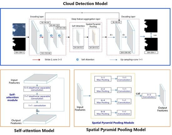
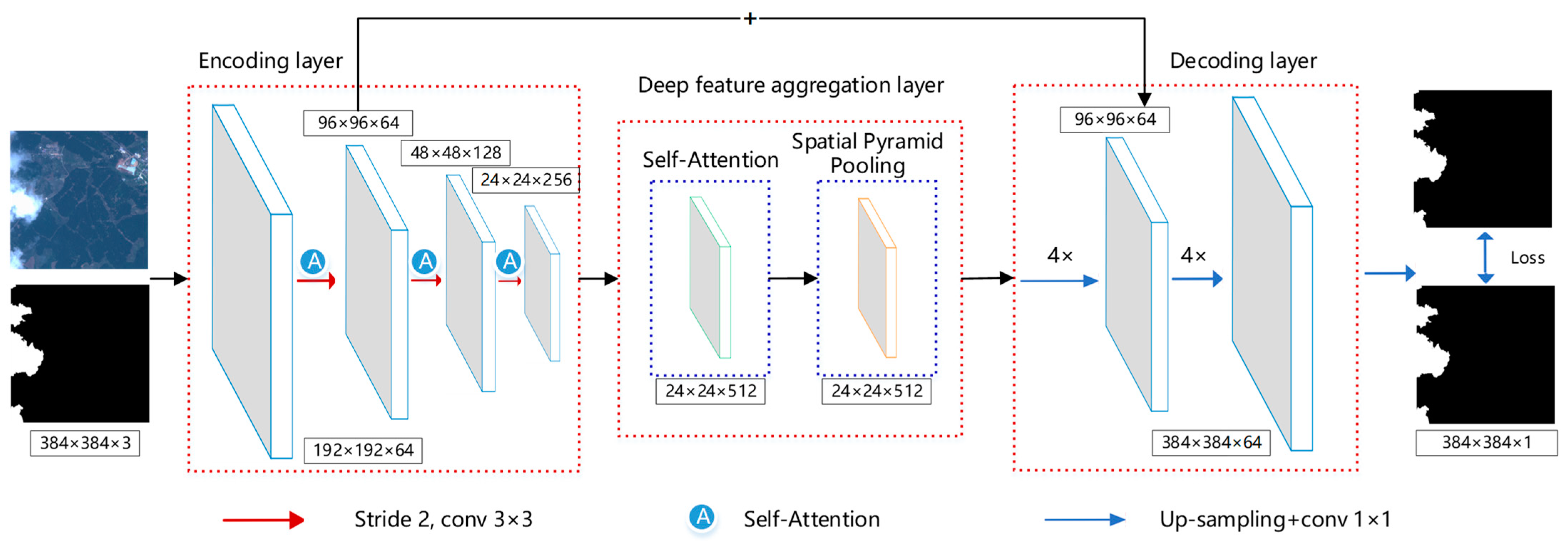
We innovatively introduce a new attention module with a large convolution kernel and design a cloud detection network model that fuses a global self-attention module with spatial pyramidal pooling, detecting and combining global features with local features to improve the detection accuracy of gauzy cloud regions and cloud pixels of edge regions.

(2)

Previous cloud detection experiments were carried out only on a single data source or a few types of sensors, while we have carried out richer cloud detection experiments on only visible three-channel images and various types of commonly used optical data, verifying the reliability and robustness of our proposed new cloud detection model.

(3)

The model design idea of our cloud detection can provide some new insights to other remote sensing image information extraction methods, such as change detection, object detection, or object extraction.

1.1. Related Work

1.1.1. Attention Module

The attention module was originally developed for natural language processing tasks [28]. The main advantage is that it can capture long-range features [29], and compared with convolution structure, the high-level semantic feature is significantly improved, thus the attention module has been applied to many downstream tasks, such as object detection [30], semantic segmentation [9], image classification [31], and instance segmentation [32]. From the method categories, the attention module can be classified into four basic categories [27] they are channel attention, spatial attention, temporal attention, and branch attention. In addition, the combination of each basic module can create some interesting new attention structures, such as spatial attention and channel attention, a classical network is DANet [21], which has achieved the highest accuracy in related semantic segmentation competitions. The main architecture of the two-way attention module consists of a Channel Attention Module (CAM) and a Position Attention Module (PAM). The channel attention layer connects different features from channels to solve the insufficient connection problem among different features in traditional CNNs and improves the global semantic connection among features. However, the two-way attention module requires high-performance hardware. To address this problem, ref. [22] proposed a novel attention module that can obtain rich semantic features for any pixel on the feature map by simply representing it with the corresponding row and column pixels, thus effectively reducing the hardware overhead and showing better results in terms of accuracy. With the newly developed transformer architecture, such as the Swin-transformer, the attention module shows a broad application prospect.

Attention module in 2D images, a common approach is to use mathematical transformation to convert 2D images into 1D sequences, though it is simple to implement, it has some problems in computer vision, especially in large remote sensing imageries. For example, the computation complexity of attention modules is very high [27], especially for high-resolution images. Another shortcoming of the attention module is that it can only achieve spatial adaptability while the channel information is missing [27]. As we know, for remote sensing images, the channel information is very important to detect different objects [33,34]. Therefore, it is important to develop a simple attention module that is lightweight and has strong adaptability for spatial and channel dimensions. Moreover, it can also maintain the property of traditional convolution structure.

1.1.2. Spatial Pyramid Pooling Module

Spatial pyramid pooling provides a good information description for overall scene interpretation [35]. It has three advantages: (1) it can solve the problem of inconsistent image size; (2) it can aggregate semantic features at different spatial scales; and (3) it can improve the accuracy of the downstream task, such as object detection or semantic segmentation [36]. A classical segmentation network architecture is DeepLab [37]. In order to solve the problem of information loss, such as downsampling in traditional convolution, dilation convolution is used in DeepLabV1 [37]. The final segmentation accuracy improves significantly, and the main idea of DeepLabV1 is that dilation convolution can keep the spatial resolution unchanged, while increasing the receptive field. DeepLabV2 proposes an atrous spatial pyramid pooling module (ASPP) to adapt to the multi-scale feature of an object [38]. In DeepLabV3 [39] and DeepLabV3+ [40], it modifies the ASPP module in DeepLabV2, and uses multiple improved parallel dilation convolution blocks to improve the segmentation accuracy. Though the ASPP module successfully applies to semantic segmentation, the dilation parameter in dilation convolution is constant. Ref. [41] propose a new module, namely “Dilated Convolution with Learnable Spacing (DCLS)”, which has a learnable parameter. The final segmentation result demonstrates that DCLS is suitable for irregular object segmentation.

Another way to aggregate multi-scale context features is to use global pooling operations, such as max-pooling or average-pooling. Ref. [35] proposes a global average pooling module to refine the pixel-level segmentation result. Though global context feature aggregation can improve the segmentation accuracy, the boundary of multi-scale objects still has a large room for improvement. Ref. [14] propose a pyramid scene parsing network. The core module is PPM, which uses four pooling operations to aggregate multi-scale high-level context features. The segmentation result shows that the accuracy in the edge area improves significantly. Another advantage of PPM is that it has high computational efficiency. The recent study by [42] also uses a simple PPM module to develop a lightweight network for real-time segmentation. Consequently, for massive optical remote sensing imageries, using PPM as a multi-scale high-level feature aggregation module is a cheap but effective alternative.

2. Materials and Methods

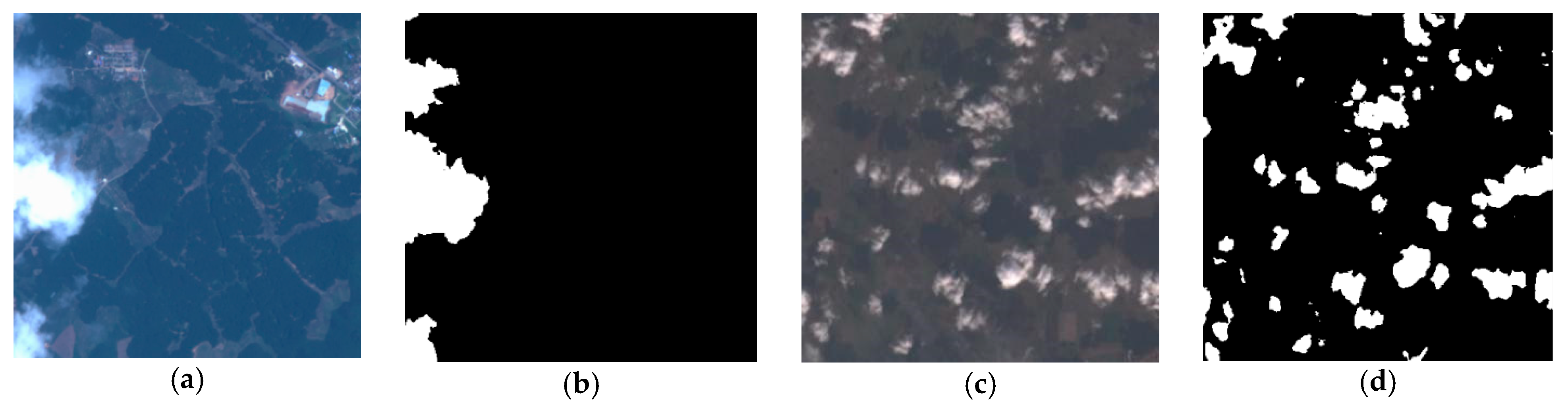
2.1. Data

It is well known that the number of samples has a significant impact on the accuracy improvement of deep learning models [43], so we used a multi-source data mixture for training. The most important advantage is to improve the model generation ability. We used two datasets: the first one was adopted from the open-source Landsat8 dataset provided by [17] (https://github.com/SorourMo/38-Cloud-A-Cloud-Segmentation-Dataset) (accessed on 6 February 2019), which contains a total of 26,301 images of a 384 × 384 size. The second dataset is the AIR-CD data [13], which is generated with the Chinese Gaofen-2 PMS data and is cropped into 384 × 384 tiles to keep pace with the Landsat8 training dataset, with a total of 10,982 sample data. In terms of spectral band selection, we kept only the RGB visible bands of both the Landsat8 dataset and the AIR-CD dataset. Some sample examples are shown in Figure 1.

Figure 1. Training images and label images. (a) GF-2 true color images. (b) GF-2 ground truth images. (c) Landsat8 true color images. (d) Landsat8 ground truth images.

The distribution of training, testing, and validation datasets are shown in Table 1:

Table 1. The proportion between training data and test data.

Data Sources	Training Set (Train Model)	Test Set (for Selecting the Optimal Model)	Validation Set (for Comparing Algorithm Accuracy)
Landsat8	15,781	5260	5260
GF-2	6590	2196	2196

To enhance the robustness of the segmentation model, we use the following data augmentation methods: (1) random angle rotation; (2) image folding; (3) random scale scaling; (4) channel confusion; (5) random brightness change. On remote sensing images, geographical features present huge spectral differences in different time-phases and regions, and the data augmentation methods mentioned above could effectively enhance the generalization ability of the model and improve the segmentation accuracy. In practical applications, such as change detection, many users abandon the NIR band and only use the visible bands. This is the main reason why we develop cloud detection methods with only RGB band input. In addition, Google Earth in the USA and Tianditu in China also only have RGB bands, and our proposed cloud detection methods can be migrated up seamlessly.

To test the generalization ability of the model, we selected multiple sensor data with different resolutions for testing. In the data preprocessing stage, only the visible RGB bands were retained with 2% linear stretching and finally converted to uint8. The relevant test data and ID are shown in Table 2.

Table 2. The metadata information of multi-source remote sensing images.

Satellite	Spatial Resolution	Data ID	Season	Topography	Land Cover Types
GF-6 WFV	16 m	GF6_WFV_E79.7_N29.1_20201230_ L1A1120067165	Winter	Plateaus, Plains	Snow, forest, grassland, cropland
GF-1 WFV	16 m	GF1_WFV2_E118.3_N49.2_20200527_L1A0004828354	Spring	Mountains	Urban, forest, cropland, shrubland
Landsat9	30 m	LC09_L2SP_178026_20220327_20220329_02_T1	Spring	Plains	Water bodies, cropland, wetlands
Beijing-2	3.2 m	PMS_L1_20201103023341_003023VI_002_0120201221002001_005	Autumn	Hills	Urban, forest, cropland
Sentinel-2	10 m	20220623T025529_20220623T031001_ T49QGE	Summer	Plains	Urban, water, cropland

2.2. Proposed Cloud Detection Module

We propose a cloud detection model that fuses the attention module with spatial pyramid pooling to effectively extract clouds from complex scenes. It mainly consists of three main parts, i.e., an encoding layer, a depth feature aggregation layer, and a decoding layer (Figure 2). The encoding layer is mainly used to extract depth features, the deep feature aggregation layer is used to extract richer semantic features, and the decoding layer is used to segment clouds by fusing multi-scale features from the encoding layer.

Figure 2. Proposed cloud detection module.

In Figure 2, the self-attention module and the spatial pyramid pooling module are two key modules, whose main purpose is to obtain richer and more effective cloud features to improve the accuracy of cloud detection in complex scenes. The implementation of the self-attention module and the pyramid pooling module is shown in Figure 3.

Figure 3. Self-attentive Module and Spatial Pyramid Pooling Module. (a) Self-Attention Module. (b) Spatial Pyramid Pooling Module.

2.3. Encoding Layer

As stated above, the encoding layer is mainly used for the deep semantic features of the image. Usually, semantic segmentation networks use ResNet18, ResNet50, and ResNet101 as backbone feature extraction networks [43]. These residual networks can effectively alleviate the gradient disappearance phenomenon and can improve models’ accuracy, but with an increased computational burden, which can seriously affect models’ inference efficiency in practical production environments. The core idea of the DenseNet network architecture [44] is borrowed from the ResNet architecture, with the main purpose of reducing the vanishing gradient that occurs during deep learning training, enhancing feature reuse, and making the features of network learning more fine-grained. The improved feature reuse with a very small number of network parameters is critical for improving training efficiency. In a single block of the DenseNet, each output layer is stacked with all the previous output layers, which directly learns the features of the previous level and improves the reuse rate. Due to the diversity of features, the feature output dimension of the next level could be reduced to reduce the computation burden of the network. Compared with other networks such as Unet [45], DenseNet focuses more on feature extraction and is less computationally intensive. With the deepening of the network, the richness of the extracted features will increase, but it will bring higher hardware overhead.

To balance accuracy and efficiency, we modify the DenseNet 121 (a variant of DenseNet) backbone network for feature extraction. Compared with the original DenseNet 121 network, we make improvements in the following two aspects: (1) for each original 384 × 384 size image block input, we only keep the network layer with a 12 × 12 size feature dimension, and discard the concatenated layer behind, and the final extracted feature dimension size is 1/32 of the original input; (2) during the forward pass of the network, each 3 × 3 convolutional downsampling module with a step size of 2 is connected to a self-attention module, with the aim to make the network learn richer semantic features.

2.4. Deep Feature Integration Layer

The deep feature integration layer contains two key modules: the self-attention module and the spatial pyramid pooling module.

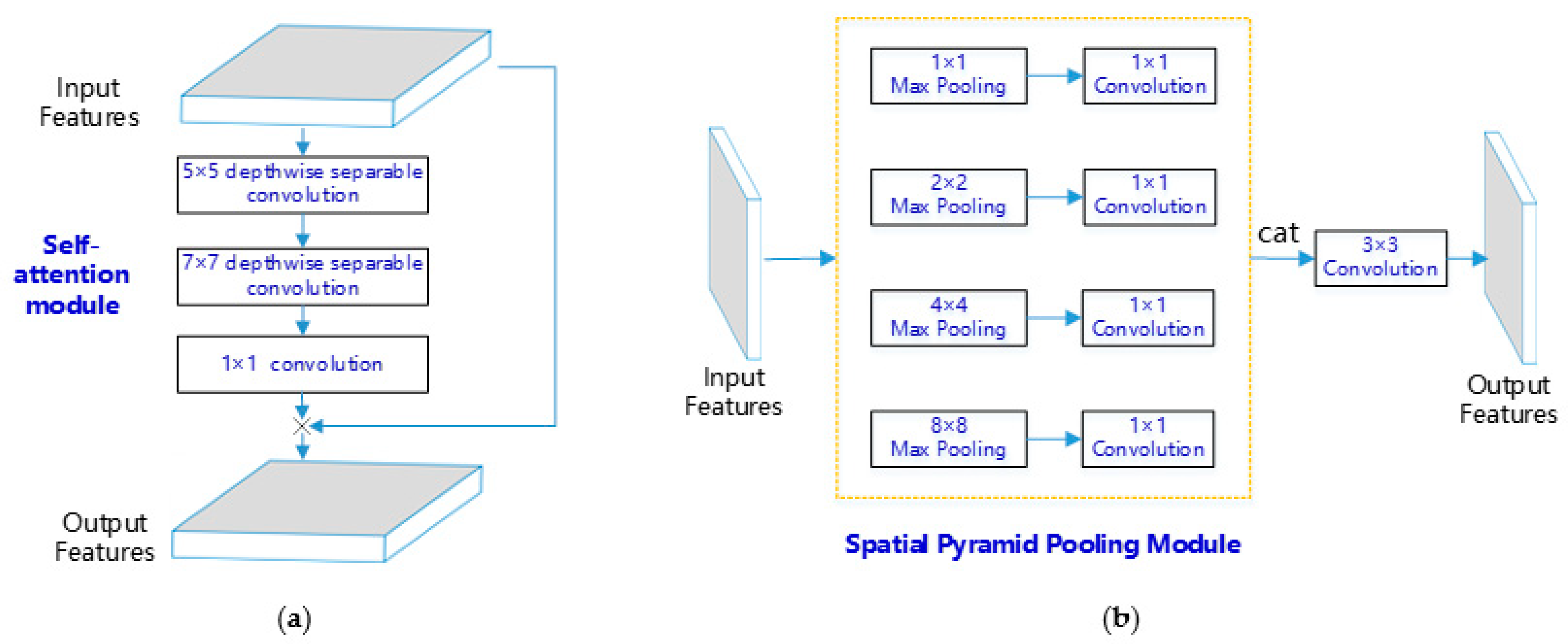
2.4.1. Proposed Self-Attention Module

The primitive self-attentive module was originally used in the field of natural language processing (NLP, natural language process) to improve the accuracy of speech recognition and has been widely adopted even in the field of image processing. Since then, varieties of the self-attention module have emerged to solve the insufficient feature learning problem that exists in traditional CNNs and to enable the network to learn more effective contextual features. Analysis of existing attention modules shows that most of them require complex matrix computation operations, which is the underlying factor causing low computational efficiency. Ref. [27] implemented a visual attention module using only a depthwise separable convolution with a large convolution kernel with array multiplication and achieved optimal results in a relevant vision task. Inspired by this work, we introduce the visual attention module into our cloud detection model to improve the detection accuracy of gauzy clouds coverage regions and cloud pixel edge regions.

2.4.2. Spatial Pyramid Pooling Module

In semantic segmentation, the contextual feature extraction of pixels has a crucial impact on the subsequent segmentation accuracy. For features of different sizes, their information obtained by a single-scale convolution module is limited, and although the ResNet module can extract richer semantic features by deepening the network depth, the computation overhead increases significantly with deeper depth, thus reducing inference efficiency. Ref. [40] proposed an atrous spatial pyramid pooling module (ASPP) to obtain contextual information of pixels in the form of atrous convolution, extracting different feature information by setting convolution blocks of different atrous scales and then fusing the features in a feature stacking (Concat) so that the network learns the feature information of different scales and effectively improves the pixel segmentation accuracy. Ref. [14] proposed a spatial pyramid pooling module (PPM) approach for feature fusion, and the core steps are feature aggregation by pooling operation, pooling parameters by setting different scales to form feature layers, and finally, feature fusion by Concat, because pooling operators do not need parameter learning [14], thus PPM has a high computing performance.

To deal with the complex forms of cloud targets of different sizes and shapes, we use the PPM module for multi-scale feature aggregation to extract the finer features of cloud targets. In the detailed implementation. The maximum pooling is used for feature aggregation the pooling parameters are set to 1,2,4,8, and then the 4-dimensional features are fused in the way of Concat to improve the segmentation accuracy of the model.

2.5. Decoding Layer

The decoding layer performs multi-scale feature fusion with the encoding layer features by up-sampling, and then an optimization function is used to optimize the final output features to finally achieve pixel-level cloud target segmentation.

2.5.1. Multi-Scale Feature Fusion

The decoding layer uses two 4 × 4 up-sampling modules to achieve feature size alignment, and after the first up-sampling module extracts the features, they are fused with the encoding layer features to fuse semantic features of different scales to achieve high precision segmentation of cloud targets of different sizes and shapes. The core idea of this architecture is borrowed from the design idea of Unet, and relevant documents [46] show that this fusion method has a good segmentation effect for small targets and complex scene targets that are very similar to cloud target segmentation, which can therefore be reasonably adopted in the current study.

2.5.2. Optimization Function

In the semantic segmentation field, cross-entropy is usually used as the loss function [9]. In practical applications, cloud targets and background targets usually have large differences in pixel ratios, and directly using cross-entropy cannot effectively balance the differences in the number of targets. To effectively solve this problem, we mend the cross-entropy function as follows:

$$bce=-(\frac{{\displaystyle \sum _{i\in Z_1}logP(y_i=1)}}{num\_pos}+\frac{{\displaystyle \sum _{i\in Z_2}log(1-P(y_i=0))}}{num\_neg})$$

(1)

where $P\left(y_i=1\right)$denotes the probability value of a positive sample pixel i after the sigmoid function, $P\left(y_i=0\right)$denotes the probability value of a negative sample pixel i after the sigmoid function, $Z_1$denotes a positive sample pixel set, $Z_2$denotes a negative sample set, $nu{m}_{-}pos$ and $nu{m}_{-}neg$ denote the pixel counts of positive and negative samples in a labeled sample set, respectively.

2.6. Accuracy Assessment

We quantitatively evaluate the model performance using the five metrics, Accuracy, Recall, Precision, F1-score, and IOU (Intersection over Union), whose formulas are:

Accuracy = (TP + TN)/(TP + TN + FP + FN)

(2)

Recall = TP/(TP + FN)

(3)

Precision = TP/(TP + FP)

(4)

F1-score = (2 × Recall × Precision)/(Recall + Precision)

(5)

IOU = TP/(TP + FP + FN)

(6)

where TP indicates that the predicted result is a cloud pixel and the ground truth pixel is also a cloud pixel. TN indicates that the predicted pixel is the background value and the ground truth pixel is also the background value. FP indicates that the pixel in the ground truth image is cloud but is predicted as the background value. FN indicates that the pixel in the ground truth image is the background value but is predicted as cloud.

3. Results

3.1. Parameter Setting

Our experimental setup consists of an AMD 5600X CPU, the Ubuntu 20.04 operating system, the Pytorch 1.10.1 deep learning framework, and an RTX 3090 with a 24 GB memory GPU. We use the Adam optimizer and set the batch size parameter to 16, the initial learning rate to 0.0001, and the epoch of training to 60.

3.2. Comparison with Feature-Based Cloud Detection Methods

To fairly evaluate the cloud detection capabilities of different algorithms, we chose the classical Fmask algorithm [6], MFC [5], and CSD-SI [7] methods for comparison. The test images were selected from a Landsat8 multispectral image (ID LC08_L1TP_116029_20131205_20170428_01_T2), where clouds and snow coexist and can effectively test the performance of different algorithms in complex scenes, and the ground truth was generated by visual interpretation. A brief description of the principle of the contrast algorithm, the optimal parameters setting of the algorithm, and the details of the bands involved in the cloud mask are shown in Table 3.

Table 3. Comparison of different feature-based algorithms.

Algorithm	Journal	Principles	Band List (Landsat8)	Reference Code Address and Parameters Setting
Fmask	RSE	For the open-sourced Landsat5-Landsat8, and Sentinel-2 data, which are widely used globally, the authors improve the differentiation between clouds and snow by introducing DEM with global surface water coverage data and combining a new spectral-contextual snow index. By conducting a large number of experimental comparisons in different regions of the world, the authors show that the method is effective and has a high practical value, and it has been used by GEE (Google Earth Engine) as the official optical data cloud masking algorithm.	Visible light (RGB) + Near-infrared (NIR) + Short wave infrared (SWIR) + Thermal infrared (TIR)	We use the official Fmask algorithm at GEE, the source code is: https://code.earthengine.google.com/361fc7a4b6d1b6817030d501b0d2b01e (accessed on 14 March 2022)
MFC	RSE	For the Chinese GF-1 WFV data, a cloud and cloud shadow detection algorithm with the fusion of spectral indices and geometric features is proposed. For the problem that it is difficult to distinguish the highlighted object from the cloud target, the authors use shape feature constraints to solve this difficult problem, and for the cloud–snow mixing region, LBP texture is used to assist in the improvement. Finally, cloud and cloud shadow detection experiments are conducted on different scenes to prove the effectiveness of the method.	Visible light (RGB) + Near-infrared (NIR)	The official software is downloaded from http://sendimage.whu.edu.cn/en/mfc/ (accessed on 1 July 2017), and the key parameters are set using the recommended settings of the paper, where the shape feature FRAC is set to 1.4, which is due to the optimal results achieved on the images used in this paper.
CSD-SI	ISPRS	Previous feature-based cloud and cloud shadow detection algorithms can only be adapted to the problem of a single sensor. The authors propose a new spectral index for detecting multispectral and hyperspectral optical image cloud and shadow targets, and the literature achieves better experimental results on different data sources such as Landsat5, Landsat7, Landsat8, and GF-1, which verifies the effectiveness and robustness of the new cloud detection feature index.	Visible light (RGB) + Near-infrared (NIR)	The algorithm was replicated using Matlab 2020b, where the T1 parameter was set to 0.02 and t2 was set to 1/4.

It is worth noting that the three algorithms mentioned above also detect shadows along with clouds. For comparison, since our model focuses on only clouds, we use only the cloud detection results of the above algorithm, and the optimal parameter settings also focus on the cloud detection effect. When using our algorithm for cloud detection, the original image is preprocessed using a 2% linear stretching, retaining only the RGB visible triplet bands without the involvement of additional band information such as the NIR and shortwave SWIR bands. The results are shown in Figure 4.

Figure 4. Comparison of cloud detection effects of different algorithms (the yellow area in the figure indicates the missed detection pixels and the blue area indicates the wrong detection pixels, the letter A represents the subregion of the whole image, we will discuss different algorithms performance in this area). (a) True color Landsat8 images. (b) ground truth. (c) Fmask. (d) MFC. (e) CSD-SI. (f) ours.

To more clearly compare the experimental effects of different algorithms, we zoom in on the sub-region A of the true-color image, as shown in Figure 5.

Figure 5. Detail comparison of different algorithms (the yellow area in the figure indicates the missed detection pixels and the blue area indicates the incorrectly detected pixels). (a) True-color image of subregion A. (b) Subregion A ground truth map. (c) Fmask algorithm cloud detection results for subregion A. (d) MFC algorithm cloud detection results for subregion A. (e) CSD-SI algorithm Cloud detection results for subregion A. (f) Our algorithm cloud detection results for subregion A.

It is obvious from Figure 5 that the deep learning method has relatively fewer false detection pixels and better visual results in the cloud–snow mixing region. The CSD-SI and MFC algorithms, on the other hand, misidentified a large number of snow-covered regions as clouds, indicating that using them for high-precision cloud–snow differentiation is more challenging as they have limited spectral features. Fmask alleviates the cloud–snow mixing false detection problem to some extent due to the inclusion of more optical features, but there is still a large number of false detection in the edge region of cloud pixels. The proposed cloud detection method based on deep learning using the RGB visible triple bands has obtained better detection results, which is more valuable for practical applications considering that more and more optical remote sensing satellites are collecting data with only RGB bands to reduce costs.

The quantitative assessment of the experimental results is shown in Table 4.

Table 4. Comparison of feature-based cloud detection methods quantitative accuracy.

Methods	Accuracy	Recall	Precision	F1-Score	IOU
Fmask	0.8351	0.8794	0.3895	0.5399	0.3693
MFC	0.7766	0.2449	0.1611	0.1943	0.1076
CSD-SI	0.8268	0.2866	0.2497	0.2669	0.1539
Proposed method	0.9419	0.8693	0.7297	0.7934	0.5865

It is obvious that the proposed cloud detection method achieved the highest accuracy in terms of all the three indices, further proving that the deep learning method can perform high-precision cloud detection using a smaller number of bands.

3.3. Comparison with Other Cloud Detection Methods Based on Deep Learning Methods

We selected DeeplabV3+ [40], MT-Unet [47] semantic segmentation networks, and cloud detection methods selected MSCFF [9], CDNet [13], RS-net [12], and GCDB-UNet [4] for comparison, and the training parameters were kept consistent with our methods. Table 5 shows the details of the comparison.

Table 5. Detailed analysis of different deep learning models.

Methods	Journal	Model Characteristics
DeeplabV3+	ECCV	This model is a semantic segmentation algorithm for natural images. The core idea is the use of a spatial pyramid pooling module to perceive object features of different scales and sizes by fusing multi-scale contextual semantic features, and the overall architecture is simple and effective, with smooth and accurate object segmentation boundaries. In our comparison experiments, ResNet50 is used as the backbone feature network to extract depth features. For the pyramid pooling module of this network, we use {1,6,12,18} as the atrous convolution parameters.
MT-Unet	ICASSP	The model is a segmentation network developed for medical images. Unlike the CNN architecture, the core module of this network is developed based on the transformer, and the overall architecture still adopts an encoder-decoder architecture similar to U-net, with the major innovation being the design of a self-attention module with local-global Gaussian adaptive weights, which makes the extracted features richer. Experiments are conducted on medical images, and the results show that the highest accuracy is achieved. Since the attention module we use is also global feature extraction, the transformer network is chosen for comparison.
MSCFF	ISPRS	This model is a cloud detection algorithm for optical remote sensing images, and its main idea is to use a segmentation network similar to the U-net architecture, and the core is similar to DeeplabV3+ in employing multi-scale expansion convolution to obtain the depth semantic features of cloud targets at different scales, which has shown good experimental accuracy in different data sources at home and abroad. In our comparison experiments, the original parameter settings are used, the last two encoding modules and the beginning two decoding modules of MSCFF, and the expansion convolution parameters are set to 2 and 4.
CDNet	TGRS	This model is a cloud detection algorithm for complex scenarios such as cloud–snow coexistence, and its main idea is to use a multi-scale feature pyramid module with a boundary optimization module, which shows high experimental accuracy on China ZY-3 images. Since the network was originally designed for thumbnail image cloud detection, we use it for the original true-color images for the sake of fairness of comparison, and the backbone features use the improved ResNet50 network from the original paper.
RS-net	RSE	This model is a cloud detection algorithm for optical remote sensing images, and its main idea is based on U-net for improvement. The authors use the cloud mask results detected by the Fmask algorithm as training samples and restart training the network model, which has higher accuracy than Fmask on the test dataset and can effectively distinguish cloud–snow mixed pixels, proving the effectiveness and robustness of deep learning methods in cloud detection.
GCDB-UNet	KBS	This model is mainly a cloud detection network developed for difficult scenarios such as gauzy clouds. The core idea is to develop a non-local attention module to model complex scenes in context, which effectively improves the detection accuracy of gauzy clouds. The authors demonstrate the effectiveness of the model by conducting experiments on the self-developed MODIS dataset.

In the above table, ECCV represents the conference of the European Conference on Computer Vision, ICASSP is the conference of the IEEE International Conference on Acoustics, Speech and Signal Processing, ISPRS means ISPRS Journal of Photogrammetry and Remote Sensing, TGRS represents IEEE Transaction on Geoscience and Remote Sensing, RSE represents Remote Sensing of Environment, and KBS is Knowledge-Based Systems.

In order to fairly evaluate the performance capability of different algorithm models in practical application scenarios, the GF-2 PMS data are selected for experimental comparison. The test data are the validation set partly divided from the AIR-CD dataset, and the lower mat contains different types of cloud–snow coexistence areas, water bodies, cities, and croplands. The image preprocessing method also uses 2% linear stretching for the original four-channel multispectral images, retaining only the RGB visible bands, and the image sizes are all 6907 × 7300 × 3. The cloud detection results of different algorithm models are shown in Figure 6.

Figure 6. Comparison of cloud detection results of different algorithms (from top to bottom, true-color image map, ground truth, DeeplabV3+ extraction result, MT-Unet, MSCFF extraction results, CDNet extraction results, RS-net, GCDB-UNet, and extraction result of our algorithm. The yellow areas indicate the missed extracted pixels and the blue areas indicate the wrong extracted pixels, the letter A/B represents the subregion of the whole picture, we will discuss different algorithms performance in this area).

In Figure 6, our proposed model has relatively better cloud detection results, with relatively fewer omission alarms, relatively fewer pixels of false negative in the gauzy cloudy region, and more accurate performance in the edge region, while the DeeplabV3+, MSCFF, and RS-net models miss relatively more pixels. The DeeplabV3+ model is a segmentation algorithm for natural images, and its dilation convolutional block uses a fixed atrous convolution scale parameter, which is {1,6,12,18}, thus is not entirely appropriate for remote sensing images as they are very sensitive to multiple spatial scales. MSCFF uses a dilation convolutional block similar to DeeplabV3+ and with a lower dilation parameter (only 2 and 4), thus in the larger cloud target region, the central region appears to be under-extracted and the network might misidentify this region as snow. From this, it can be concluded that obtaining global semantic features can get better results. The cloud pixel regions extracted by GCDB-UNet with the attention module are more accurate, which is due to the long-range feature modeling capability of the attention module, but there are still many false predictions in the cloud pixel edge regions, which may be because the model does not perform reinforcement feature learning for the edge pixels. Although MT-Unet adopts a local-global self-attentive module, it is essentially a segmentation network developed for medical images. On medical images, the contextual information is often simple and the network does not need to be deep, but it is sensitive to long-range features. For cloud targets on remote sensing images, the shape, brightness, and contextual information are extremely different, and a shallower network may not be able to learn the complex semantic information, resulting in more false alarms, and the same problem is found with RS-net. To better compare the differences in the extraction results of different algorithms, we zoom into a local area in the above figure, as shown in Figure 7.

Figure 7. Detail comparison of different deep learning models at subregioin A (the yellow areas indicate missed extracted pixels and the blue areas indicate wrongly extracted pixels). (a) True color images. (b) ground truth. (c) DeeplabV3+. (d) MT-Unet. (e) MSCFF. (f) CDNet. (g) RS-net cloud. (h) GCDB-Unet. (i) ours.

A comparison of the effect of cloud detection in subregion B is shown in Figure 8.

Figure 8. Detail comparison of different deep learning models at subregion B (the yellow areas indicate the missed extracted pixels and the blue areas indicate the wrong extracted pixels). (a) True color images. (b) ground truth. (c) DeeplabV3+. (d) MT-Unet. (e) MSCFF. (f) CDNet. (g) RS-net. (h) GCDB-Unet. (i) ours.

From Figure 8, it can be seen that the cloud regions detected by DeeplabV3+ have more false recognition cases, MSCFF and MT-Unet cloud detection results miss more pixels, CDNet and GCDB-Unet network cloud detection is relatively good, but in the edge part, the false pixels still occupy a certain proportion. The RS-net cloud detection results all have partial omissions and false detections. From the local experimental comparison, our algorithm extracts relatively better results, especially in the cloud edge and gauzy cloud coverage regions. In terms of implementation theory, our cloud detection network uses a large convolutional kernel for feature extraction and then global pixel modeling to extract features from arbitrary pixels. Compared with the previous attention module, the attention to the edge area and the gauzy cloud coverage area of the feature extraction will be stronger, which directly shows that the effect of cloud detection in this complex area is more satisfactory, and the central “window area” of large thick clouds can be effectively distinguished.

The results of the quantitative evaluation of the extraction results of GF-2 are shown in Table 6.

Table 6. Comparison of deep learning based cloud detection methods quantitative accuracy.

Methods	Accuracy	Recall	Precision	F1-Score	IOU
DeeplabV3	0.90386	0.8754	0.8543	0.8647	0.7614
MT-Unet	0.8856	0.9312	0.7836	0.8511	0.7407
MSCFF	0.8857	0.8750	0.8135	0.8431	0.7288
CDNet	0.9051	0.9961	0.7891	0.8806	0.7867
RS-net	0.8275	0.7719	0.7456	0.7585	0.6110
GCDB-UNet	0.8915	0.9970	0.7650	0.8657	0.7632
Proposed method	0.9375	0.9868	0.8568	0.9172	0.8471

As can be seen from Table 6, our accuracy is relatively better with an F1-score, proving that the attention module employing a large convolutional kernel is effective and reasonable for the cloud detection task.

4. Discussion

4.1. Ablation Study

To objectively evaluate the impact of different modules on the accuracy, we used ablation experiments to verify the degree of contribution of different modules in the model to the overall accuracy. The GF-2 data from the previous section were selected for quantitative accuracy evaluation, and the results are shown in Table 7, where the backbone model refers to the removal of the PPM and self-attention modules, and the training parameters are kept consistent.

Table 7. Ablation study.

Module Selection	Accuracy	Recall	Precision	F1-Score	IOU
backbone model	0.8642	0.8541	0.8265	0.8400	0.7551
+PPM	0.9038	0.9173	0.8378	0.8757	0.8097
+self-attention	0.9281	0.9459	0.8408	0.8902	0.8259
+PPM+self-attention	0.9375	0.9868	0.8568	0.9172	0.8417

From Table 7, we can see that the self-attention module has the greatest improvement in the accuracy performance of the model, and the spatial pyramid pooling module also has some improvement, and both of them are successively combined to achieve the highest cloud detection accuracy, indicating that the deep feature aggregation layer is effective.

From the experimental results, the deep learning method outperforms the multi-band thresholding method in terms of accuracy, despite only using the RGB visible bands, verifying the effectiveness and universality of the deep learning method. Compared with other deep learning methods, our cloud detection model, in terms of detail performance, is better, with relatively fewer missed and incorrectly detected pixels, especially in the thin cloud coverage area and cloud pixel boundary area, and the visual effect is also relatively better. From the network implementation theory, our cloud detection model mainly adopts the self-attentive module and spatial pyramid pooling for feature fusion, which are essentially extracted deep features with a larger range and richer semantics to improve the accuracy of cloud detection in complex regions.

4.2. Generalization Ability Discussion

To test the generation ability of our proposed module, we use the multi-source remote sensing images in Table 2. The cloud detection results are shown in Figure 9.

Figure 9. Cloud detection results of multi-source remote sensing imagery (the yellow areas indicate the missed extracted pixels and the blue areas indicate the wrong extracted pixels). (a) GF-1 WFV true color images. (b) ground truth. (c) cloud detection results. (d) GF-6 WFV true color images. (e) ground truth. (f) cloud detection results. (g) Landsat9 true color images. (h) ground truth. (i) cloud detection results. (j) Beijing-2 true-color images. (k) ground truth. (l) cloud detection results. (m) Sentinel-2 true-color images. (n) ground truth. (o) cloud detection result.

It can be very clearly seen that our cloud detection model has equally effective generalization ability on a variety of images such as GF-1 WFV, GF-6 WFV, Landsat9, Beijing-2, etc. The quantitative accuracy evaluation is shown in Table 8.

Table 8. Quantitative accuracy of multi-source remote sensing images.

Image Data Source	Spatial Resolution (m)	Image Size (Pix)	Accuracy	Recall	Precision	F1-Score	IOU
GF-1 WFV	16	13,400 × 12,000 × 3	0.9733	0.9093	0.9203	0.9147	0.8913
GF-6 WFV	16	17,797 × 12,817 × 3	0.9861	0.9187	0.9370	0.9278	0.9153
Landsat9	30	7761 × 7861 × 3	0.9822	0.9574	0.9988	0.9777	0.9563
Beijing-2	3.2	7815 × 7260 × 3	0.9977	0.9277	0.9458	0.9366	0.9261
Sentinel-2	10	10,922 × 10,940	0.9828	0.9449	0.9090	0.9266	0.9197

In Table 8, the overall accuracy of the F1-Score is above 0.9, which proves the generalization ability of the model. In addition, a very interesting point is that the cloud detection model performs with higher accuracy on the latest Landsat9 images relative to the other image data, and a more detailed comparison from the visual aspect also reveals that the edge regions are more accurate, probably due to the Landsat8 imagery used for the training samples. Landsat8 and Landsat9 are very similar in terms of optical and spatial resolution indicators, which potentially makes the models more sensitive to similar data. This is useful for large-scale cloud detection practical application tasks, which can be trained with similar data or similar data sources according to the optical characteristics and spatial resolution of the target image. This idea is not only valid for the task of cloud detection but also still holds theoretically for other geographic feature extraction and classification tasks.

4.3. Efficiency Discussion

In real-world scenarios, the efficiency of cloud detection algorithms is also a very important indicator. In order to compare the computational efficiency of different algorithms, we tested GF-1WFV data (shown in Section 4.2) with RTX3090 as the test hardware GPU, and the models were not subjected to any pruning, quantization, or other acceleration operations. Conversely, the trained model files are directly used for inference. The consumption times of different models are shown in Table 9.

Table 9. Comparison of the computational efficiency of different deep learning model.

Algorithm	Time-Consuming (s)
DeeplabV3	19.03
MT-Unet	18.71
MSCFF	28.21
CDNet	25.98
RS-net	19.29
GCDB-UNet	26.37
Proposed algorithm	16.08

It can be seen that our computational efficiency reaches the relative optimum. Furthermore, thanks to the hardware optimization (NVIDIA GPU), the efficiency of the deep learning method is very high. A large image with 13,400 × 12,000 × 3 pixels only need 16s to generate cloud mask. Therefore, on a mass of optical remote sensing images in real-world scenarios, we can produce cloud mask layers with cloud detection methods based on deep learning. In addition, to effectively improve the efficiency of cloud mask preprocessing by other research works, we have developed an automated cloud detection tool that can be downloaded from https://github.com/wzp8023391/Cloud-Detection-Tool.git (accessed on 18 March 2022).

5. Conclusions

In this manuscript, we proposed a new cloud detection model. Compared with other deep learning-based cloud detection methods, it achieves the optimum accuracy. Moreover, the computation efficiency is also faster. With the help of a large convolution kernel (such as 7 × 7 convolution), more efficient semantic features can be captured by our new cloud detection model. To our best knowledge, our proposed model is the first one to use a large kernel to detect clouds in optical remote sensing images. Consequently, it also gives us some new inspiration for remote sensing interpretation, that is, researchers can use large kernels and are not limited to the small kernel (3 × 3). In addition, we innovatively use a data mixed training method of multi-source remote sensing images with different spatial resolutions. Interestingly, in training a cloud detection model in this way, the model still indicates strong robustness and stability. Moreover, when the input image has the same or similar spatial resolution as the training samples, the detection accuracy is more accurate. Thus, in order to improve the robustness of deep learning models in remote sensing images, a cheap method is to increase the quantity of training samples of different spatial resolutions, and that is also our next research focus.

References

- Li, J.F.; Wang, L.Y.; Liu, S.Q.; Peng, B.A.; Ye, H.P. An automatic cloud detection model for Sentinel-2 imagery based on Google Earth Engine. Remote Sens. Lett. 2022, 13, 196–206. [Google Scholar] [CrossRef]
- Luo, C.; Feng, S.S.; Yang, X.F.; Ye, Y.M.; Li, X.T.; Zhang, B.Q.; Chen, Z.H.; Quan, Y.L. LWCDnet: A Lightweight Network for Efficient Cloud Detection in Remote Sensing Images. IEEE Trans. Geosci. Remote Sens. 2022, 60, 5409816. [Google Scholar] [CrossRef]
- Zhang, H.D.; Wang, Y.; Yang, X.L. Cloud detection for satellite cloud images based on fused FCN features. Remote Sens. Lett. 2022, 13, 683–694. [Google Scholar] [CrossRef]
- Li, X.; Yang, X.F.; Li, X.T.; Lu, S.J.; Ye, Y.M.; Ban, Y.F. GCDB-UNet: A novel robust cloud detection approach for remote sensing images. Knowl.-Based Syst. 2022, 238, 107890. [Google Scholar] [CrossRef]
- Li, Z.; Shen, H.; Li, H.; Xia, G.; Gamba, P.; Zhang, L. Multi-feature combined cloud and cloud shadow detection in GaoFen-1 wide field of view imagery. Remote Sens. Environ. 2017, 191, 342–358. [Google Scholar] [CrossRef]
- Qiu, S.; Zhu, Z.; He, B. Fmask 4.0: Improved cloud and cloud shadow detection in Landsats 4–8 and Sentinel-2 imagery. Remote Sens. Environ. 2019, 231, 111205. [Google Scholar] [CrossRef]
- Zhai, H.; Zhang, H.; Zhang, L.; Li, P. Cloud/shadow detection based on spectral indices for multi/hyperspectral optical remote sensing imagery. ISPRS J. Photogramm. Remote Sens. 2018, 144, 235–253. [Google Scholar] [CrossRef]
- Satpathy, A.; Jiang, X.D.; Eng, H.L. LBP-Based Edge-Texture Features for Object Recognition. IEEE Trans. Image Process. 2014, 24, 1953–1964. [Google Scholar] [CrossRef]
- Li, Z.; Shen, H.; Cheng, Q.; Liu, Y.; You, S.; He, Z. Deep learning based cloud detection for medium and high resolution remote sensing images of different sensors. ISPRS J. Photogramm. Remote Sens. 2019, 150, 197–212. [Google Scholar] [CrossRef]
- Wei, J.; Huang, W.; Li, Z.Q.; Sun, L.; Zhu, X.L.; Yuan, Q.Q.; Liu, L.; Cribb, M. Cloud detection for Landsat imagery by combining the random forest and superpixels extracted via energy-driven sampling segmentation approaches. Remote Sens. Environ. 2020, 248, 112005. [Google Scholar] [CrossRef]
- Abdar, M.; Pourpanah, F.; Hussain, S.; Rezazadegan, D.; Liu, L.; Ghavamzadeh, M.; Nahavandi, S. A review of uncertainty quantification in deep learning: Techniques, applications and challenges. Inf. Fusion 2021, 76, 243–297. [Google Scholar] [CrossRef]
- Jeppesen, J.H.; Jacobsen, R.H.; Inceoglu, F.; Toftegaard, T.S. A cloud detection algorithm for satellite imagery based on deep learning. Remote Sens. Environ. 2019, 229, 247–259. [Google Scholar] [CrossRef]
- Yang, J.Y.; Guo, J.H.; Yue, H.J.; Liu, Z.H.; Hu, H.F.; Li, K. CDnet: CNN-Based Cloud Detection for Remote Sensing Imagery. IEEE Trans. Geosci. Remote Sens. 2019, 57, 6195–6211. [Google Scholar] [CrossRef]
- Zhao, H.; Shi, J.; Qi, X.; Wang, X.; Jia, J. Pyramid scene parsing network. In Proceedings of the IEEE Conference on Computer Vision and Pattern Recognition, Honolulu, HI, USA, 21–26 July 2017; pp. 2881–2890. [Google Scholar]
- He, Q.B.; Sun, X.; Yan, Z.Y.; Fu, K. DABNet: Deformable Contextual and Boundary-Weighted Network for Cloud Detection in Remote Sensing Images. IEEE Trans. Geosci. Remote Sens. 2022, 60, 5601216. [Google Scholar] [CrossRef]
- Li, H.; Xiong, P.; Fan, H.; Sun, J. DFANet: Deep Feature Aggregation for Real-Time Semantic Segmentation. In Proceedings of the 2019 IEEE/CVF Conference on Computer Vision and Pattern Recognition (CVPR), Long Beach, CA, USA, 15–20 June 2019; pp. 9514–9523. [Google Scholar]
- Mohajerani, S.; Saeedi, P. Cloud-Net: An End-to-End Cloud Detection Algorithm for Landsat 8 Imagery. In Proceedings of the 2019 IEEE International Geoscience and Remote Sensing Symposium (IGARSS 2019), Yokohama, Japan, 28 July–2 August 2019; pp. 1029–1032. [Google Scholar]
- Wu, X.; Shi, Z.W.; Zou, Z.X. A geographic information-driven method and a new large scale dataset for remote sensing cloud/snow detection. ISPRS J. Photogramm. Remote Sens. 2021, 174, 87–104. [Google Scholar] [CrossRef]
- Zhang, J.; Zhou, Q.; Wu, J.; Wang, Y.C.; Wang, H.; Li, Y.S.; Chai, Y.Z.; Liu, Y. A Cloud Detection Method Using Convolutional Neural Network Based on Gabor Transform and Attention Mechanism with Dark Channel Subnet for Remote Sensing Image. Remote Sens. 2020, 12, 3261. [Google Scholar] [CrossRef]
- Zhang, J.; Wu, J.; Wang, H.; Wang, Y.C.; Li, Y.S. Cloud Detection Method Using CNN Based on Cascaded Feature Attention and Channel Attention. IEEE Trans. Geosci. Remote Sens. 2022, 60, 4104717. [Google Scholar] [CrossRef]
- Fu, J.; Liu, J.; Tian, H.J.; Li, Y.; Bao, Y.J.; Fang, Z.W.; Lu, H.Q. Dual Attention Network for Scene Segmentation. In Proceedings of the 2019 IEEE/CVF Conference on Computer Vision and Pattern Recognition (CVPR 2019), Long Beach, CA, USA, 15–20 June 2019; pp. 3141–3149. [Google Scholar]
- Huang, Z.L.; Wang, X.G.; Huang, L.C.; Huang, C.; Wei, Y.C.; Liu, W.Y. CCNet: Criss-Cross Attention for Semantic Segmentation. In Proceedings of the IEEE/CVF International Conference on Computer Vision (ICCV), Seoul, Korea, 27–28 October 2019; pp. 603–612. [Google Scholar]
- Lv, N.; Zhang, Z.H.; Li, C.; Deng, J.X.; Su, T.; Chen, C.; Zhou, Y. A hybrid-attention semantic segmentation network for remote sensing interpretation in land-use surveillance. Int. J. Mach. Learn. Cybern. 2022, 1, 1–12. [Google Scholar] [CrossRef]
- Qing, Y.H.; Huang, Q.Z.; Feng, L.Y.; Qi, Y.Y.; Liu, W.Y. Multiscale Feature Fusion Network Incorporating 3D Self-Attention for Hyperspectral Image Classification. Remote Sens. 2022, 14, 742. [Google Scholar] [CrossRef]
- Jamali, A.; Mahdianpari, M. Swin Transformer and Deep Convolutional Neural Networks for Coastal Wetland Classification Using Sentinel-1, Sentinel-2, and LiDAR Data. Remote Sens. 2022, 14, 359. [Google Scholar] [CrossRef]
- Ding, X.; Zhang, X.; Zhou, Y.; Han, J.; Ding, G.; Sun, J. Scaling Up Your Kernels to 31x31: Revisiting Large Kernel Design in CNNs. arXiv 2022, arXiv:2203.06717. [Google Scholar]
- Guo, M.-H.; Lu, C.-Z.; Liu, Z.-N.; Cheng, M.-M.; Hu, S.-M. Visual attention network. arXiv 2022, arXiv:2202.09741. [Google Scholar]
- Vaswani, A.; Shazeer, N.; Parmar, N.; Uszkoreit, J.; Jones, L.; Gomez, A.N.; Polosukhin, I. Attention is all you need. Adv. Neural Inf. Process. Syst. 2017, 30. Available online: https://proceedings.neurips.cc/paper/2017/file/3f5ee243547dee91fbd053c1c4a845aa-Paper.pdf (accessed on 14 July 2022).
- Lee, J.D.M.C.K.; Toutanova, K. Pre-training of deep bidirectional transformers for language understanding. arXiv 2018, arXiv:1810.04805. [Google Scholar]
- Yuan, Y.; Huang, L.; Guo, J.; Zhang, C.; Chen, X.; Wang, J. Ocnet: Object context network for scene parsing. arXiv 2018, arXiv:1809.00916. [Google Scholar]
- Chen, C.F.R.; Fan, Q.; Panda, R. Crossvit: Cross-attention multi-scale vision transformer for image classification. In Proceedings of the IEEE/CVF International Conference on Computer Vision, Montreal, BC, Canada, 11–17 October 2021; pp. 357–366. [Google Scholar]
- Sun, Y.; Gao, W.; Pan, S.; Zhao, T.; Peng, Y. An efficient module for instance segmentation based on multi-level features and attention mechanisms. Appl. Sci. 2021, 11, 968. [Google Scholar] [CrossRef]
- Chen, L.C.; Papandreou, G.; Kokkinos, I.; Murphy, K.; Yuille, A.L. DeepLab: Semantic image segmentation with deep convolutional nets, atrous convolution, and fully connected CRFs. IEEE Trans. Pattern Anal. Mach. Intell. 2017, 40, 834–848. [Google Scholar] [CrossRef]
- Qin, Z.; Zhang, P.; Wu, F.; Li, X. Fcanet: Frequency channel attention networks. In Proceedings of the IEEE/CVF International Conference on Computer Vision, Montreal, BC, Canada, 11–17 October 2021; pp. 783–792. [Google Scholar]
- Liu, W.; Rabinovich, A.; Berg, A.C. Parsenet: Looking wider to see better. arXiv 2015, arXiv:1506.04579. [Google Scholar]
- Zhao, L.; Dong, X.; Chen, W.Y.; Jiang, L.F.; Dong, X.J. The combined cloud model for edge detection. Multimed. Tools Appl. 2017, 76, 15007–15026. [Google Scholar] [CrossRef]
- Chen, L.C.; Papandreou, G.; Kokkinos, I.; Murphy, K.; Yuille, A.L. Semantic image segmentation with deep convolutional nets and fully connected CRFs. arXiv 2014, arXiv:1412.7062. [Google Scholar]
- Chen, L.; Zhang, H.; Xiao, J.; Nie, L.; Shao, J.; Liu, W.; Chua, T.S. SCA-CNN: Spatial and channel-wise attention in convolutional networks for image captioning. In Proceedings of the IEEE Conference on Computer Vision and Pattern Recognition, Honolulu, HI, USA, 21–26 July 2017; pp. 5659–5667. [Google Scholar]
- Chen, L.C.; Papandreou, G.; Schroff, F.; Adam, H. Rethinking atrous convolution for semantic image segmentation. arXiv 2017, arXiv:1706.05587. [Google Scholar]
- Chen, L.-C.; Zhu, Y.; Papandreou, G.; Schroff, F.; Adam, H. Encoder-Decoder with Atrous Separable Convolution for Semantic Image Segmentation. In Proceedings of the European Conference on Computer Vision (ECCV), Munich, Germany, 8–14 September 2018; pp. 833–851. [Google Scholar]
- Hassani, I.K.; Pellegrini, T.; Masquelier, T. Dilated convolution with learnable spacings. arXiv 2021, arXiv:2112.03740. [Google Scholar]
- Peng, J.; Liu, Y.; Tang, S.; Hao, Y.; Chu, L.; Chen, G.; Ma, Y. PP-LiteSeg: A Superior Real-Time Semantic Segmentation Model. arXiv 2022, arXiv:2204.02681. [Google Scholar]
- He, K.M.; Zhang, X.Y.; Ren, S.Q.; Sun, J. Deep Residual Learning for Image Recognition. In Proceedings of the 2016 IEEE Conference on Computer Vision and Pattern Recognition (CVPR), Las Vegas, NV, USA, 27–30 June 2016; pp. 770–778. [Google Scholar]
- Huang, G.; Liu, Z.; van der Maaten, L.; Weinberger, K.Q. Densely Connected Convolutional Networks. In Proceedings of the 30th IEEE Conference on Computer Vision and Pattern Recognition (CVPR 2017), Honolulu, HI, USA, 21–26 July 2017; pp. 2261–2269. [Google Scholar]
- Ronneberger, O.; Fischer, P.; Brox, T. U-Net: Convolutional Networks for Biomedical Image Segmentation. Med. Image Comput. Comput.-Assist. Interv. 2015, 9351 Pt III, 234–241. [Google Scholar]
- Yuan, Y.; Rao, F.; Lang, H.; Lin, W.; Zhang, C.; Chen, X.; Wang, J. HRFormer: High-Resolution Transformer for Dense Prediction. arXiv 2021, arXiv:2110.09408. [Google Scholar]
- Wang, H.; Xie, S.; Lin, L.; Iwamoto, Y.; Han, X.-H.; Chen, Y.-W.; Tong, R. Mixed transformer u-net for medical image segmentation. In Proceedings of the ICASSP 2022-2022 IEEE International Conference on Acoustics, Speech and Signal Processing (ICASSP), Singapore, 23–27 May 2022; pp. 2390–2394. [Google Scholar]
Publisher’s Note: MDPI stays neutral with regard to jurisdictional claims in published maps and institutional affiliations. |
© 2022 by the authors. Licensee MDPI, Basel, Switzerland. This article is an open access article distributed under the terms and conditions of the Creative Commons Attribution (CC BY) license (https://creativecommons.org/licenses/by/4.0/).