Article

Underwater Image Restoration via Contrastive Learning and a Real-World Dataset †

1
Data 61, Commonwealth Scientific and Industrial Research Organisation (CSIRO), Canberra 2601, Australia
2
College of Engineering & Computer Science, Australian National University, Canberra 2601, Australia
3
Oceans & Atmosphere, Commonwealth Scientific and Industrial Research Organisation (CSIRO), Canberra 2601, Australia
*
Author to whom correspondence should be addressed.
This paper is an extended version of our paper published in International Geoscience and Remote Sensing Symposium (IGARSS), Brussels, Belgium, 11–16 July 2021.
Remote Sens. 2022, 14(17), 4297; https://doi.org/10.3390/rs14174297
Submission received: 26 July 2022 / Revised: 16 August 2022 / Accepted: 21 August 2022 / Published: 31 August 2022

Abstract

:
Underwater image restoration is of significant importance in unveiling the underwater world. Numerous techniques and algorithms have been developed in recent decades. However, due to fundamental difficulties associated with imaging/sensing, lighting, and refractive geometric distortions in capturing clear underwater images, no comprehensive evaluations have been conducted with regard to underwater image restoration. To address this gap, we constructed a large-scale real underwater image dataset, dubbed Heron Island Coral Reef Dataset (‘HICRD’), for the purpose of benchmarking existing methods and supporting the development of new deep-learning based methods. We employed an accurate water parameter (diffuse attenuation coefficient) to generate the reference images. There are 2000 reference restored images and 6003 original underwater images in the unpaired training set. Furthermore, we present a novel method for underwater image restoration based on an unsupervised image-to-image translation framework. Our proposed method leveraged contrastive learning and generative adversarial networks to maximize the mutual information between raw and restored images. Extensive experiments with comparisons to recent approaches further demonstrate the superiority of our proposed method. Our code and dataset are both publicly available.

Graphical Abstract

1. Introduction

For marine science and oceanic engineering, significant applications such as the surveillance of coral reefs, underwater robotics, and submarine cable inspection require clear underwater images. For high-level computer vision tasks [1], clear underwater images are also required. Furthermore, clear images help the development of undersea remote sensing techniques [2,3,4]. Raw images with low visual quality do not meet these expectations, where the clarity of raw images is degraded by both absorption and scattering [5,6,7]. The clarity of underwater images thus plays an essential role in scientific missions. Therefore, fast, accurate, and effective techniques producing clear underwater images need to be developed to improve the visibility, contrast, and color properties of underwater images for satisfactory visual quality and practical usage. The main techniques to infer clear images are known as underwater image enhancement and restoration. Underwater image enhancement aims to produce visually pleasing results, focusing on enhancing contrast and brightness. In comparison, underwater image restoration is based on the image formulation model [5,6,7], and aims to rectify the distorted colors to present the true colors of the underwater scene. In this paper, we mainly focus on the objective of underwater image restoration.
In the underwater scene, visual quality is greatly affected by light refraction, absorption, and scattering. For instance, underwater images usually have a green-bluish tone since red light with longer wavelengths attenuates faster. Underwater image restoration is a highly ill-posed problem, which requires several parameters (e.g., global background light and medium transmission map) that are mostly unavailable in practice.
These parameters can be roughly estimated by employing priors and supplementary information; we refer to these approaches as the conventional methods. Most conventional underwater restoration methods employ priors to estimate the unknown parameters in the imaging model. The Dark Channel Prior (DCP) [8] is a simple yet effective prior for image dehazing. With the same imaging model, some variants based on the DCP have been developed for underwater imaging [5,9,10]. Carlevaris et al. [5] exploited the differences between attenuation among three color channels as a prior to predict the transmission map of the underwater scene. Drews et al. [9] ignored the red channel and proposed the Underwater Dark Channel Prior (UDCP). The UDCP applies DCP to the blue and green channels only to predict the transmission map. The Red channel prior [10] makes use of the red channel, i.e., the color associated with the longest wavelengths, to restore the underwater image.
Chiang et al. [11] employed measured attenuation coefficients of open ocean waters and assumed that the transmission map of the red channel is the recovered transmission by which the underwater image can be restored. In contrast to [9], which focused on the green and blue channels, Lu et al. [12] ignored the green channel and restored the underwater image by leveraging the transmission map estimated from the blue and red channels only. Peng et al. [13] proposed a method based on image blurriness and light absorption (IBLA), which uses a depth estimation approach to restore underwater images. Relying on the Jerlov water types [14], Berman et al. [15] took spectral profiles of water types into account to simplify underwater image restoration as image dehazing. However, due to the diversity of water types and lighting conditions, conventional underwater image restoration methods can fail to rectify the color of underwater images.
Supplementary information including polarization filters, stereo imaging, and the range map of the scene also helps underwater image restoration. Polarimetric imaging [16,17,18] relies on the polarization camera to capture the polarization information, thus removing the backscattering light effect. Stereo imaging naturally provides the range information to simplify the estimation of parameters [15].
Another approach to underwater image restoration employs learning-based methods. Recent advances in deep learning have demonstrated dramatic success in different fields. In the line of learning-based underwater image restoration, Cao et al. [19] recovered the scene radiance based on estimated background light and the scene depth using two neural networks. Barbosa et al. [20] employed the DehazeNet [21] to predict the transmission map, thus predicting the scene radiance. The underwater residual convolutional neural network (URCNN) [22] is a residual convolutional neural network. It learns the transmission map to restore the image. After restoration, it also enhances the restored image. The underwater convolutional neural network (UWCNN) [23] is a supervised model including three densely connected building blocks [24] trained on its synthetic underwater image datasets.
Although learning-based methods have demonstrated their effectiveness in modeling the underwater image restoration process, they require a large-scale dataset for training, which is often difficult to obtain. Thus, most learning-based models, regardless of enhancement or restoration, either use a limited number of real underwater images [15,25,26], synthesized underwater images [19,20,22,23,27,28,29], or natural in-air images [29,30] as either the source domain or target domain of the training set. Four commonly used underwater image restoration datasets are as follows:
  • SQUID (http://csms.haifa.ac.il/profiles/tTreibitz/datasets/ambient_forwardlooking/index.html, accessed on 25 July 2022) [15]: The Stereo Quantitative Underwater Image Dataset includes 57 stereo pairs from four different sites, two in the Red Sea and the other two in the Mediterranean Sea. Every image contains multiple color charts and its range map without providing the reference images.
  • TURBID (http://amandaduarte.com.br/turbid/, accessed on 25 July 2022) [26]: TURBID consists of five different subsets of degraded images with its respective ground-truth reference image. Three subsets are publicly available: they are degraded by milk, deepblue, and chlorophyll. Each subset contains 20, 20, and 42 images, respectively.
  • UWCNN Synthetic Dataset (https://li-chongyi.github.io/proj_underwater_image_synthesis.html, accessed on 25 July 2022) [23]: UWCNN synthetic dataset contains ten subsets, each subset representing one water type with 5000 training images and 2495 validation images. The dataset is synthesized from the NYU-v2 RGB-D dataset [31]. The first 1000 clean images are used to generate the training set and the remaining 449 clean images are used to generate the validation set. Each clean image is used to generate five images based on different levels of atmospheric light and water depth.
  • Sea-thru dataset (http://csms.haifa.ac.il/profiles/tTreibitz/datasets/sea_thru/index.html, accessed on 25 July 2022) [32]: This dataset contains five subsets, representing five diving locations. It contains 1157 images in total; every image is with its range map. Color charts are available within the partial dataset. No reference images are provided.
The above datasets are limited in capturing the natural variability in a wide range of water types. The synthetic training data also limit the generalization of models [33]. For unsupervised methods, natural in-air images are also a good source to learn from [30]; however, unsupervised methods usually lack strong constraints and thus networks may inadvertently learn the structure and geometry information of in-air images and thus tend to perform geometric changes instead of color correction.
Furthermore, only partial datasets provide reference restored images. Lacking a large-scale, publicly available real-world underwater image restoration dataset with scientifically restored images limits the development of learning-based underwater image restoration methods.
To overcome the previously discussed challenges, we constructed a large-scale real-world underwater image dataset, the Heron Island Coral Reef Dataset (HICRD). The HICRD contains 9676 raw underwater images in total and 2000 scientifically restored reference images. It contains two subsets, the unpaired HICRD and the paired HICRD. It also contains the measured diffuse attenuation coefficient and the camera sensor response.
To fully use the proposed HICRD, we designed a learning-based underwater image restoration model trained on the HICRD. We formulate the restoration problem as an image-to-image translation problem and propose a novel Contrastive underwater Restoration approach (CWR). CWR combines both contrastive learning [34,35] and generative adversarial networks [36]. Given an underwater image as input, CWR directly outputs a restored image, showing the real color of underwater objects as if the image was taken in-air without any structure or content loss. The flowchart of this paper is presented in Figure 1.
The main contribution of our work is summarized as follows:
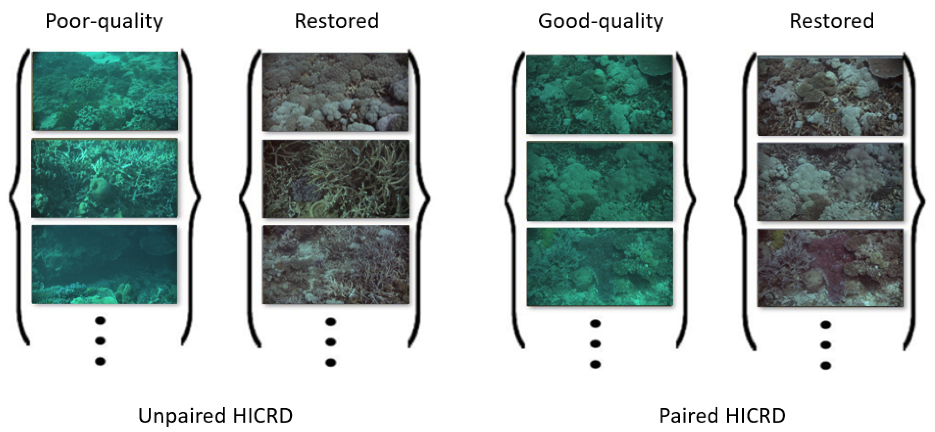
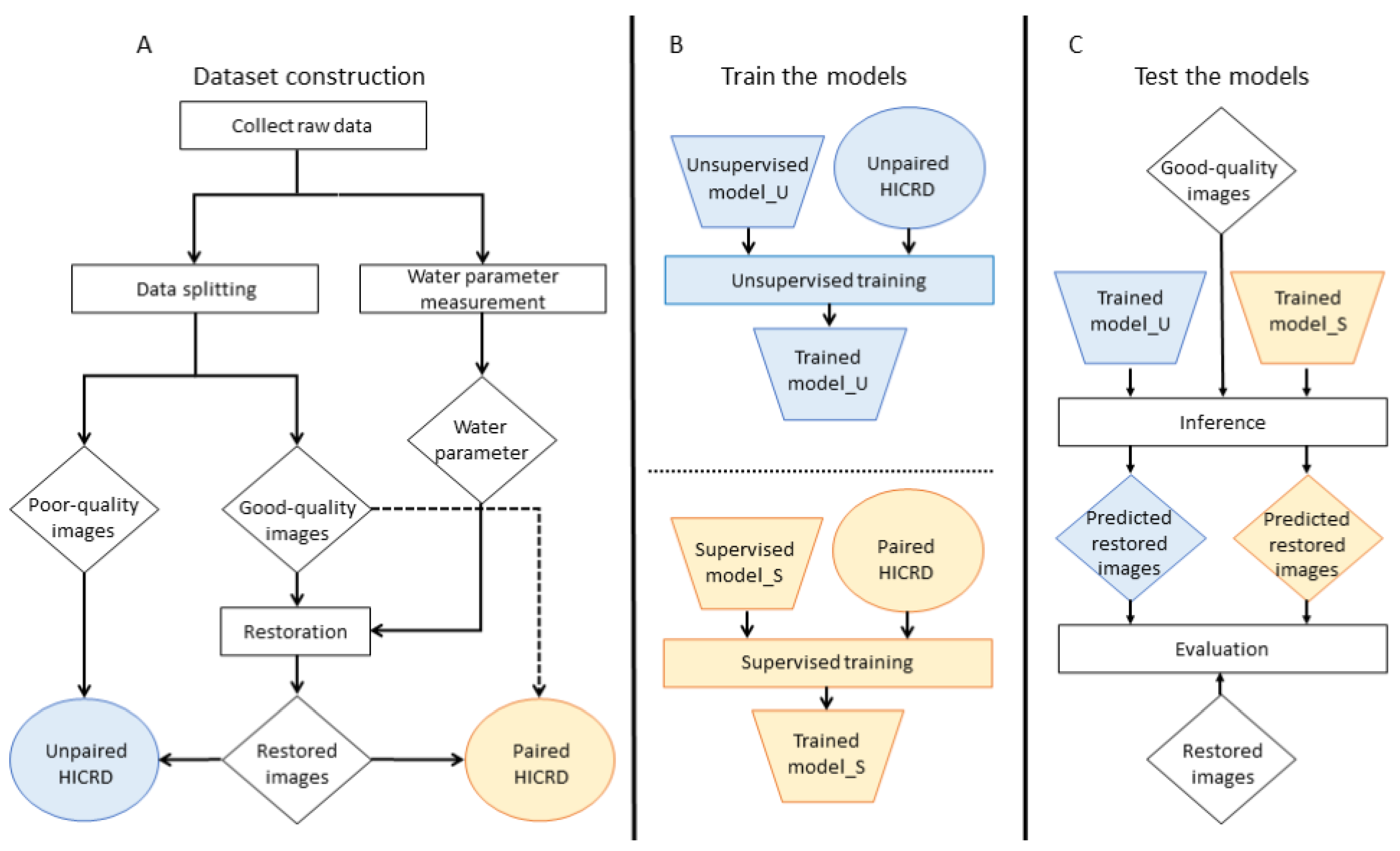
  • We constructed a large-scale, high-resolution underwater image dataset with real underwater images and restored images. The Heron Island Coral Reef Dataset (HICRD) provides a platform to evaluate the performance of various underwater image restoration models on real underwater images with various water types. It also enables the training of both supervised and unsupervised underwater image restoration models.
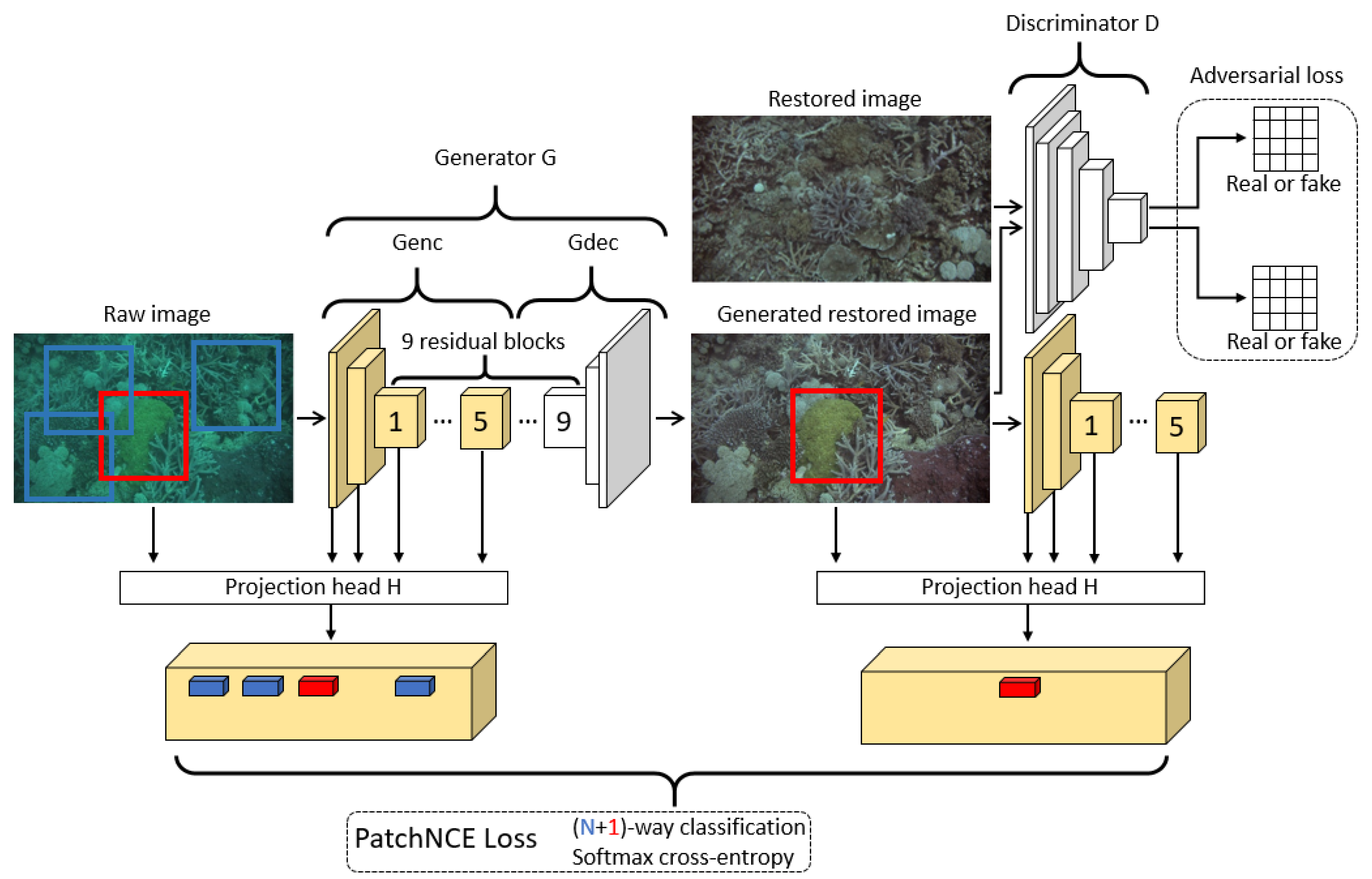
  • We proposed an unsupervised learning-based model, i.e., CWR, which leverages contrastive learning to maximize the mutual information between the corresponding patches of the raw image and the restored image to capture the content and color feature correspondences between the two image domains.
Some results of this paper were originally published in its conference version [37]. However, this longer article includes the details of the HICRD and CWR to provide a deeper understanding, e.g., data collection (Section 2.1.1), water parameter measurement (Section 2.1.2), and implementation details of CWR (Section 2.3). We also added more related work in the introduction (Section 1). A more comprehensive experiment is available in the result section (Section 3), including more baselines (Section 3.1), more evaluation results (Section 3.4), transfer learning results (Section 3.5), and an ablation study (Section 3.6). A discussion section (Section 4) is added to provide a comprehensive analysis and future research directions.

2. Materials and Methods

2.1. A Real-World Dataset

To address a previously discussed issue and gap, we collected a new dataset, measured the water parameters, and created reference restored images. In this section, we elaborate on the constructed dataset in detail, including data collection, water parameter measurement, imaging model, and reference image generation. The flowchart of this section is shown in Figure 1A.

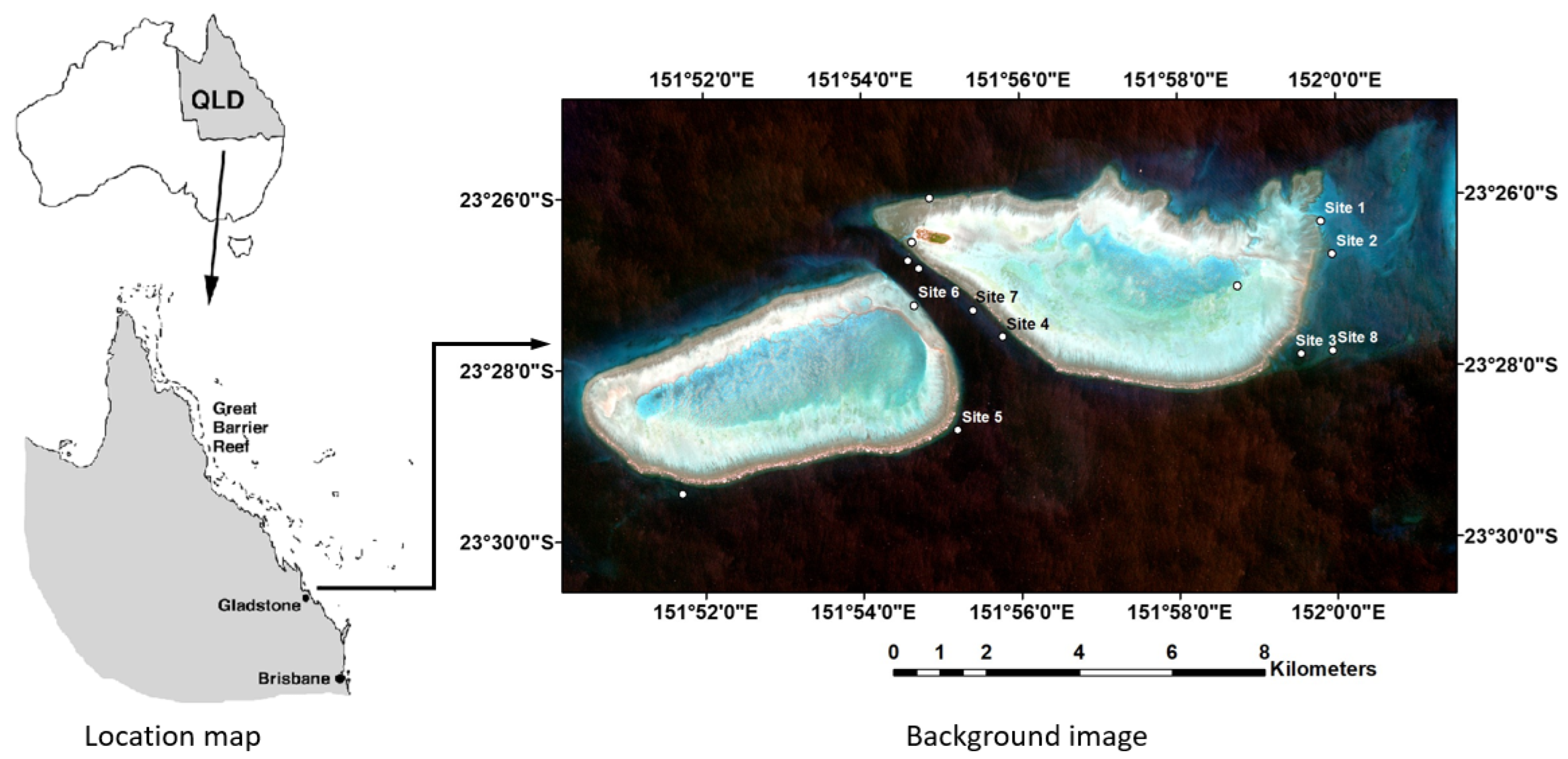
2.1.1. Data Collection

Images and other forms of optical data of HICRD were collected from several sample locations around Heron Reef, located in the Southern Great Barrier Reef, Australia, from 11 to 16 June 2018. These sample locations, corresponding to Reef Check Australia permanent transect sites [38], were selected to represent a variety of coral reef environments with a range of coral densities, water depths, and water conditions. Figure 2 shows the location of sample stations on Heron Reef and nearby Wistari Reef.
The image acquisition of HICRD was conducted using CSIRO’s Underwater Spectral Instrument Platform (CORYCAEUS). RGB images in HICRD were captured by the on-board MQ022CG-CM color camera. It is a small form factor USB 3.0 camera made by Ximea GmbH, Münster, Germany. The camera carries a 2/3″ 10-bit CMOSIS CMV 2000 sensor. The optics is an Edmund Optics 12mm focal length F1.8 lens. This lens has a field of view of 41.1 when used with the Ximea camera. During image capturing procedures, the camera aperture was fixed, and its exposure time was adjusted by a human operator on board the boat viewing the live video streamed back from the cameras while divers were swimming underwater. The image capturing frequency was 3–5 frame/s.
Our data acquisition task was accomplished by a team of divers and boat members. The divers carried out underwater data collection using CORYCAEUS. Boat staff made surface measurements, provided safety monitoring, and maintained boat control. The detailed procedure is as follows: upon arrival at a coral reef sample site, first the boat crew verify the GPS location and collect water samples, surface reflectance, water column spectral absorbance, and backscattering measurements. One then turns on CORYCAEUS and carries it to the divers. Diver one first measures underwater reflectance. Diver two then manipulates CORYCAEUS to swim in a fixed direction keeping a constant distance of 2 m above the reef. Diver one safeguards diver 2 during the whole measuring transect. Meanwhile, one of the boat members monitors the live video from CORYCAEUS transferred by a tethering cable. The boat crew follow the divers in the boat motoring at a low speed, and maintain a safe distance of (10–30 m) from the divers. At the end of each transect, the boat crew signal the divers to the surface. Both divers and CORYCAEUS are retrieved from the water. Final readings of the GPS position and other measurements are recorded.

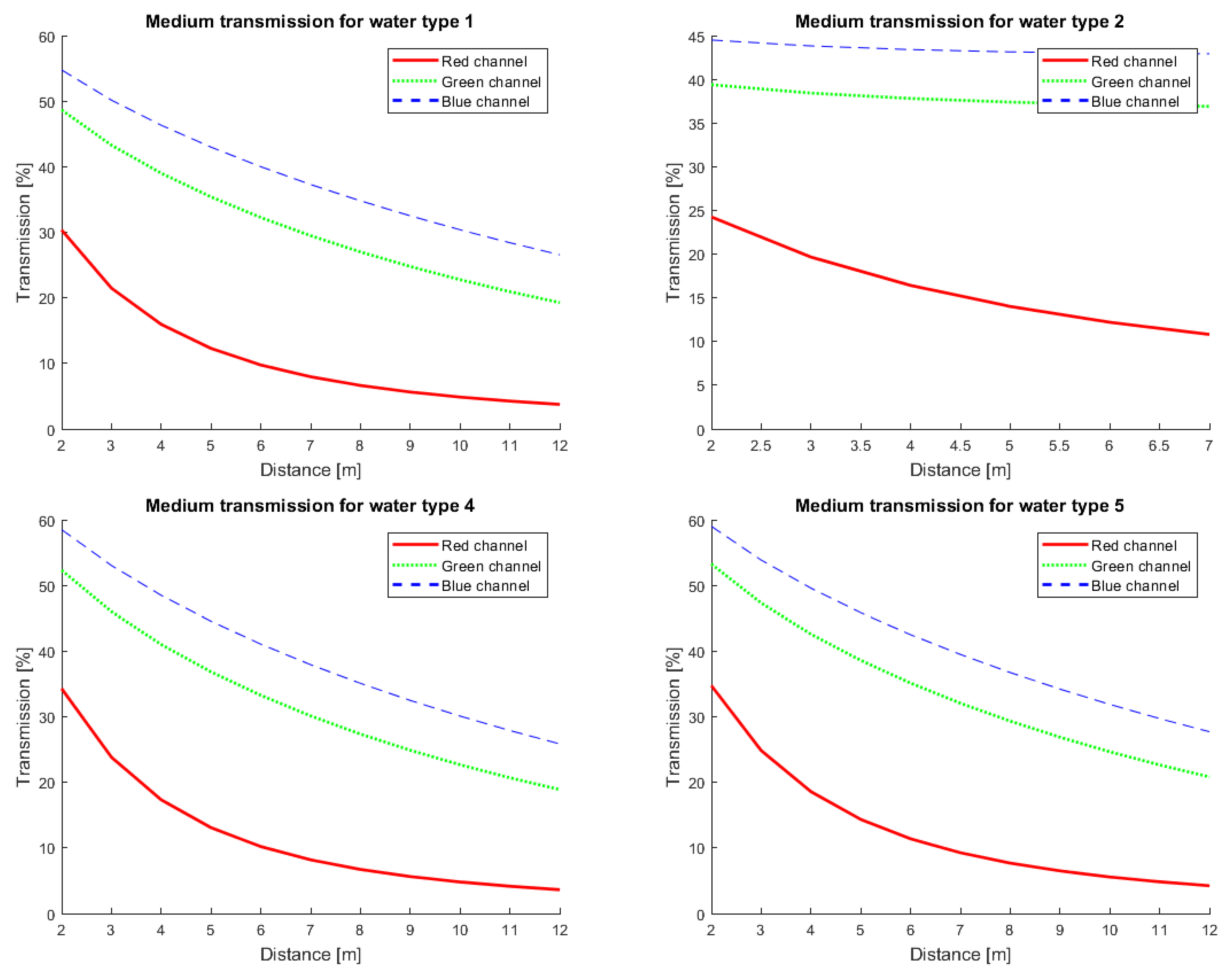
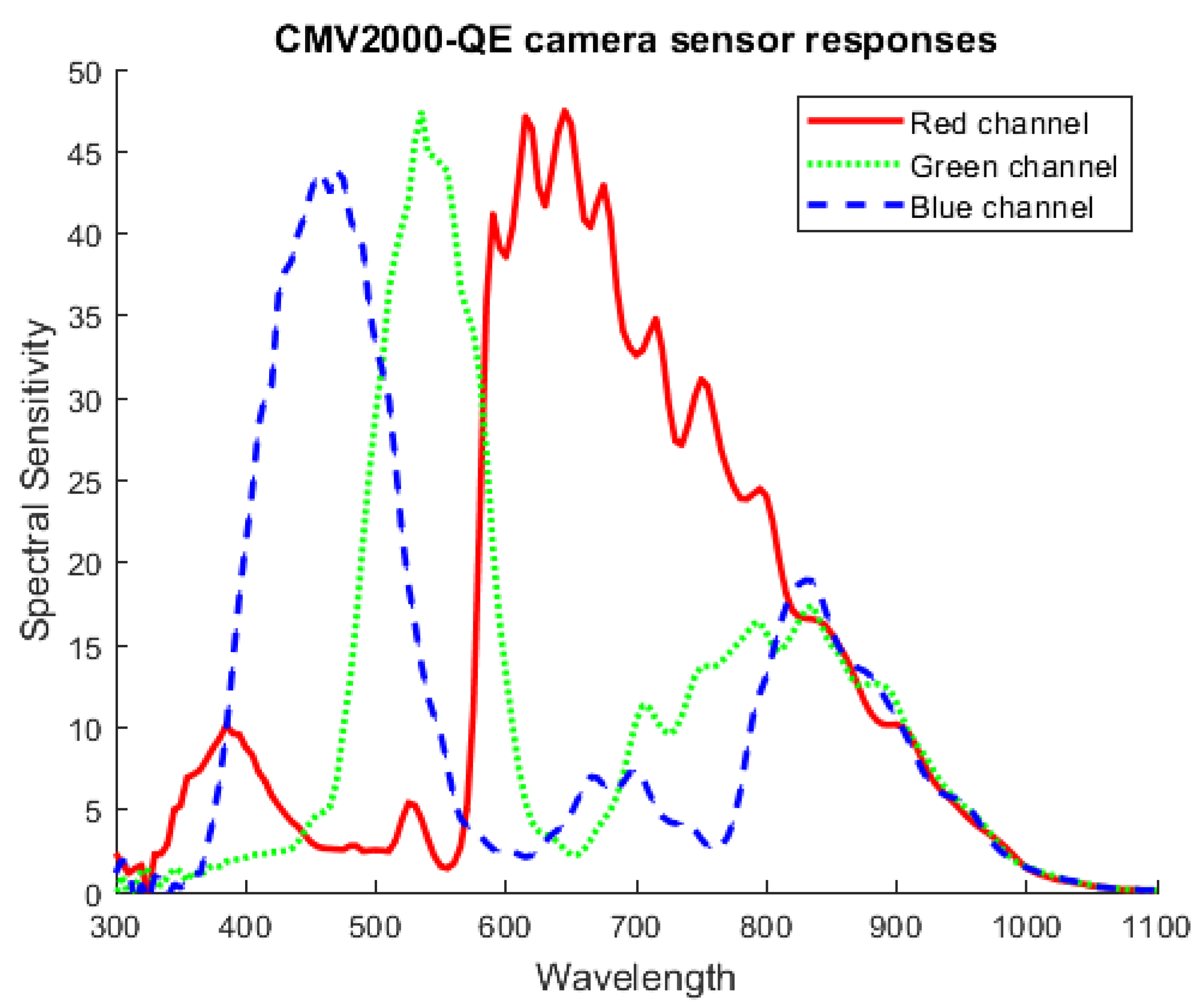
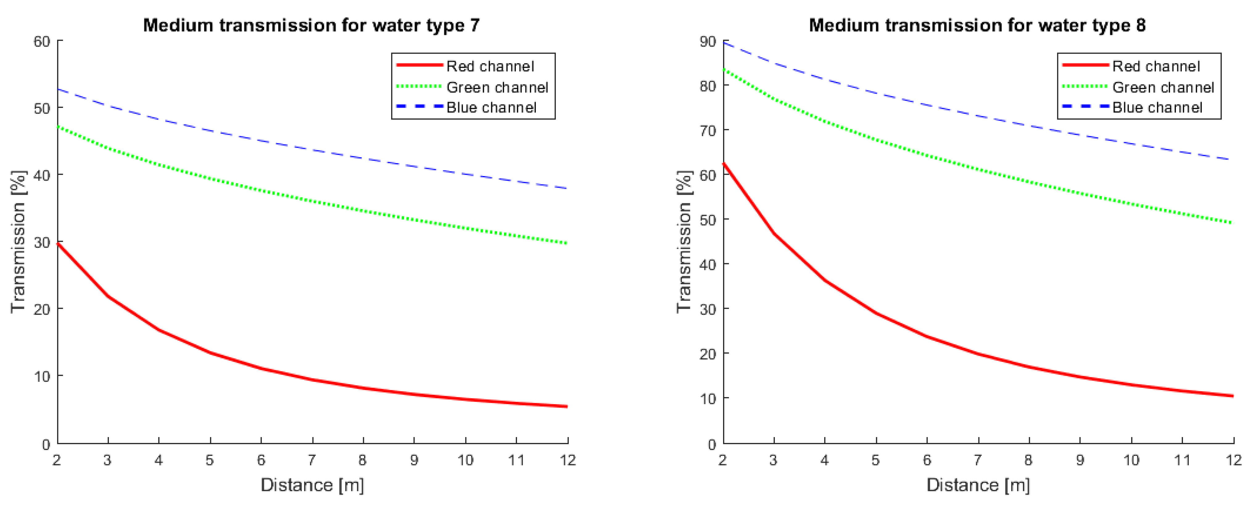
2.1.2. Water Parameter Estimation

To understand the effects of bio-optical constituents on the behavior of light through the water column, data were collected to characterize the inherent and apparent optical properties (IOPs and AOPs).
At each dive site, IOPs were collected as vertical profiles of the absorption a( λ ), and attenuation spectral coefficients c( λ ) were measured using a 10 cm path length WET Labs (http://seabird.com, accessed on 25 July 2022) spectral absorption–attenuation meter. Backscattering coefficients bb( λ ) were measured using a WET Labs BB-9 spectral backscattering meter, while temperature, salinity, and density were collected using a WET Labs water quality monitor (WQM). Profiles were measured with all instruments connected to a WET Labs DH-4 data logger, allowing consistent time stamping. The backscattering measurements were corrected for salinity and light loss due to absorption over the path length using the absorption and scattering values from the ac-s [40].
Surface water samples were collected for a laboratory analysis of the absorbing components (particulate and dissolved). Samples for particulate absorption (phytoplankton and non-algal) were prepared by filtration through a 25 mm Whatman GF/F glass-fiber filter and stored flat in liquid nitrogen for transport. Particle absorption coefficients were measured over the 250–800 nm spectral range with a Cintra 4040 UV/VIS dual-beam spectrophotometer (http://gbcsci.com, accessed on 25 July 2022) equipped with an integrating sphere [41]. Samples for a measurement of chromophoric dissolved organic matter (CDOM) absorption were prepared by vacuum filtration through a 0.22 µm Millipore filter and preserved with sodium azide for sample transport [42]. The absorbance of each filtrate was measured from 250 to 800 nm in a 10 cm pathlength quartz cell using a Cintra 4040 UV/VIS spectrophotometer [41]. Total absorption is considered as the sum of the particulate and dissolved components plus that of pure water.
Radiometric profiles (AOPs) were measured at each station using three TriOS Ramses radiometers (http://trios.de, accessed on 25 July 2022). One irradiance radiometer was mounted on the boat to measure the total downwelling irradiance, and two sensors were mounted on an underwater frame to measure the water radiance and irradiance, respectively. The diffuse attenuation coefficient ( K d ) was determined from measurements of the rate of change (slope) of the logarithm of the irradiance (E)depth profile [43] and can be written as:
K d = 1 z z 0 l n [ E ( z ) E ( z 0 ) ]
where z 0 is the uppermost depth of measurement. Depth averaged K d over the depth interval from the surface to depth z is expressed as [44]:
K d ( 0 z ) = 0 z K d ( z ) d z z

2.1.3. Detailed Information of HICRD

The Heron Island Coral Reef Dataset (HICRD) contains raw underwater images from eight sites with detailed metadata for each site, including water parameters (diffuse attenuation), maximum dive depth, and the camera model. Six sites have wavelength-dependent attenuation within the water column. According to the depth information of raw images and the distance between objects and the camera, images with roughly the same depth, constant distance, and good visual quality are labeled as good quality. Images with sharp depth changes, distance changes, or poor visual quality are labeled as low-quality. We apply our imaging model described in Section 2.1.4 to good quality images, producing corresponding reference restored images, and manually remove some restored images with non-satisfactory quality.
The HICRD contains 6003 low-quality images, 3673 good-quality images, and 2000 reference restored images. We used low-quality images and restored images as the unpaired training set. In contrast, the paired training set contains 1700 good-quality images and corresponding restored images. The test set contains 300 good-quality images as well as 300 corresponding restored images as reference images. All images are in 1842 × 980 resolution. Figure 3 shows the total diffuse attenuation for different water types. Figure 4 shows a randomly selected image examples from the HICRD and the split of the HICRD. Table 1 presents the detailed information of the HICRD. Based on the Underwater Image Quality Measure (UIQM) [45], Natural Image Quality Evaluator (NIQE) [46], and dubbed Blind/Referenceless Image Spatial Quality Evaluator (BRISQUE) [47], Table 2 presents a comparison between low-quality images and good-quality images.

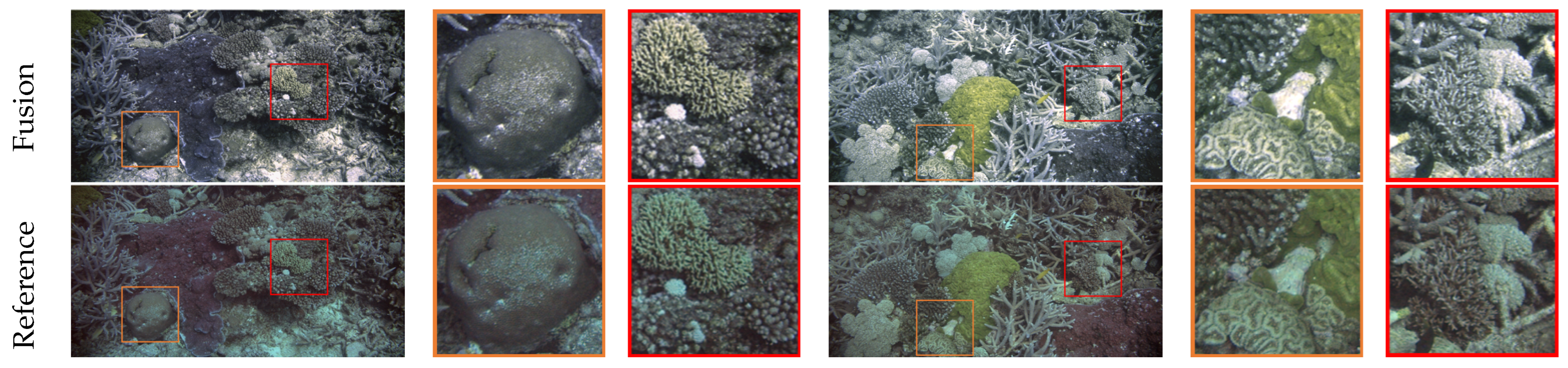
2.1.4. Underwater Imaging Model and Reference Image Generation

Unlike the dehazing model [8], absorption plays a critical role in an underwater scenario. Each channel’s absorption coefficient is wavelength dependent, being the highest for red and the lowest for blue. A simplified underwater imaging model [48] can be formulated as:
I c ( x ) = J c ( x ) t c ( x ) + A c ( 1 t c ( x ) ) , c { r , g , b } ,
where I ( x ) is the observed intensity, J ( x ) is the scene radiance, and A is the global atmospheric light. t c ( x ) = e β c d ( x ) is the medium transmission describing A ( x ) the portion of light that is not scattered, β c is the light attenuation coefficient and d ( x ) is the distance between the camera and object. Channels are in RGB space. We assume the measured diffuse attenuation coefficient K d c to be identical to the attenuation coefficient β c .
Transmittance is highly related to β c , which is the light attenuation coefficient of each channel, and it is wavelength-dependent. Unlike in previous work [11,13], instead of assigning a fixed wavelength for each channel containing bias (e.g., 600 nm, 525 nm, and 475 nm for red, green, and blue), we employed the camera sensor response to conduct a more accurate estimation. Figure 5 shows the camera sensor response of camera sensor type CMV2000-QE used in collecting the dataset.
The new total attenuation coefficient is estimated by:
p c = a b β λ S c ( λ ) d λ ,
where p c is the total attenuation coefficient, β λ is the attenuation coefficient of each wavelength, and S c ( λ ) is the camera sensor response of each wavelength. Following the human visible spectrum, we set a = 400 nm and b = 750 nm to calculate the medium transmission for each channel. We modified the medium transmission t c ( x ) in Equation (3) leading to a more accurate estimation:
t c ( x ) = e p c d ( x ) .
It is challenging to measure the scene’s actual distance from an individual image without a depth map. Instead of using a flawed estimation approach, we assumed the distance between the scene and the camera to be small (1–5 m) and manually assigned a distance for each good-quality image. The assigned distance is verified via the following process: for each water type (diving location), we checked the difference inside the image triplets (last image, current image, and next image) to ensure that the assigned distance is reasonable and consistent between images that are close to each other. If the difference is more than 1 m, this triplet will be further checked to avoid labeling noise.
The global atmospheric light, A c , is usually assumed to be the pixel’s intensity with the highest brightness value in each channel. However, this assumption often fails due to the presence of artificial lighting and self-luminous aquatic creatures. Since we have access to the diving depth, we can define A c as follows:
A c = e p c z ,
where p c is the total attenuation coefficient and z is the diving depth.
With the medium transmission and global atmospheric light, we can recover the scene radiance. The final scene radiance J ( x ) is estimated as:
J c ( x ) = I c ( x ) A c m a x ( t c ( x ) , t 0 ) + A c .
Typically, we choose t 0 = 0.1 as a lower bound. In practice, due to the complexity with image formulation, our imaging model based on the simplified underwater imaging model may encounter information loss, i.e., the pixel intensity values of J c ( x ) are larger than 255 or less than 0. This problem is avoided by only mapping a selected range (13–255) of pixel intensity values from I to J. However, outliers may still occur; we re-scale the whole pixel intensity values to enhance contrast and keep information lossless after restoration.

2.2. Proposed Method

Given two domains X R H × W × 3 and Y R H × W × 3 and a dataset of unpaired instances X containing raw underwater images x and Y containing restored images y. We denote it X = x X and Y = y Y . We aim to learn a mapping G : X Y to enable underwater image restoration.
Contrastive Underwater Restoration (CWR) has a generator G as well as a discriminator D. G enables the mapping from domain X to domain Y and D ensures that the translated images belong to the correct image domain. The first half of the generator is defined as an encoder, while the second half is a decoder and denoted G e n c and G d e c , respectively.
For the mapping, we extracted the features of images from several layers of the encoder and send them to a two-layer MLP projection head. Such a projection head learns to project the extracted features from the encoder to a stack of features. CWR combines three losses, including Adversarial loss, PatchNCE loss, and Identity loss. Figure 6 shows the overall architecture and losses of CWR. The details of our objective are described below.

2.2.1. Adversarial Loss

Generative adversarial network (GAN) [36] incorporates a generator and a discriminator, where the generator aims to generate realistic samples while the discriminator is designed to classify real samples from generated fake samples. Such an adversarial training mechanism forces generated samples to match the distribution of real samples. In our case, adversarial loss helps the generator translate raw underwater images into visually similar images into images from the target domain, that is, the domain of restored underwater images. For the mapping G : X Y with discriminator D, the GAN loss [36] is calculated by:
GAN G , D , X , Y = E y Y log D ( y ) + E x X log 1 D ( G ( x ) ) ,
where G tries to generate images G ( x ) that look similar to images from domain Y, while D aims to distinguish between translated samples G ( x ) and real samples y.

2.2.2. PatchNCE Loss

Our goal is to maximize the mutual information between corresponding patches of the input and the output. For instance, for a patch showing a coral reef of the generated restored image, we should be able to associate it more strongly to the same coral reef patch of the raw input underwater image other than the rest of the patches of the image.
Following the setting of CUT [49], we used a noisy contrastive estimation framework to maximize the mutual information between inputs and outputs. The idea behind contrastive learning is to correlate two signals, i.e., the “query” and its “positive” example, in contrast to other examples in the dataset (referred to as “negatives”).
We map query, positive, and N negatives to K-dimensional vectors and denote them v , v + R K and v R N × K , respectively. Note that v n R K denotes the n-th negative. We set up an ( N + 1 ) -way classification problem and computed the probability that a “positive” is selected over “negatives”. Mathematically, this can be expressed as a cross-entropy loss which is computed by:
v , v + , v = log ( exp s i m ( v , v + ) / τ exp s i m ( v , v + ) / τ + n = 1 N exp s i m ( v , v n ) / τ ) ,
where sim ( u , v ) = u v / u v denotes the cosine similarity between u and v . τ denotes a temperature parameter to scale the distance between the query and other examples, and we use 0.07 as default. We set the numbers of negatives as 255 as the default setting.
We used G e n c and a two-layer projection head H to extract features from domain X. We select L layers from G e n c ( X ) and send them to H, embedding one image into a stack of features z l L = H l G enc l ( x ) L , where G enc l represents the output of l-th selected layers. For the patches, after having a stack of features, each feature actually represents one patch from the image. We take advantage of that and denote the spatial locations in each selected layer as s { 1 , . . . , S l } , where S l is the number of spatial locations in each layer. We selected a query each time, referring to the corresponding feature (“positive”) as z l s R C l and all other features (“negatives”) as z l S s R S l 1 × C l , where C l is the number of channels in each layer. We have aimed to match the corresponding patches of input and output images. The patch-based, multi-layer PatchNCE loss for mapping G : X Y can be expressed as:
PatchNCE ( G , H , X ) = E x X l = 1 L s = 1 S l z ^ l s , z l s , z l S s .

2.2.3. Identity Loss

In order to prevent generators from unnecessary changes and keep the structure identical after translation, we add an identity loss [50].
Identity ( G ) = E y Y G ( y ) y 1 .
Such an identity loss also encourages the mappings to preserve color composition between the input and output.

2.2.4. Full Objective

The generated restored image should be realistic ( G A N ), and patches in the corresponding input raw and generated restored images should share a correspondence ( PatchNCE ). The generated restored image should have an identical structure to the input raw image. In contrast, the colors are the true colors of scenes ( Identity ). The full objective is:
( G , D , H ) = λ G A N G A N ( G , D , X ) + λ N C E PatchNCE ( G , H , X ) + λ i d t Identity ( G ) .
We set λ G A N = 1 and λ N C E = 1 following previous mutual information maximization methods [49,51]. We set λ i d t = 10 to prevent generators from unnecessary structure and color changes.

2.3. Implementation Details

2.3.1. Architecture of Generator and Layers Used for PatchNCE Loss

Figure 6 represents the architecture of the generator and layers used for computing PatchNCE loss. Our generator architecture is based on CycleGAN [50] and CUT [49]. We use a ResNet-based [52] generator with nine residual blocks for training. It contains two downsampling blocks, nine residual blocks, and two upsampling blocks. Each downsampling and upsampling block follows two-stride convolution/deconvolution, normalization and an activation function, i.e., ReLU. Each residual block contains convolution, normalization, ReLU, convolution, normalization, and a residual connection.
We define the first half of generator G as an encoder represented as G e n c . The patch-based multi-layer PatchNCE loss is computed using features from five layers of the encoder (the RGB pixels, the first and second downsampling convolution, and the first and the fifth residual block). The patch sizes extracted from these four layers are 1 × 1, 9 × 9, 15 × 15, 35 × 35, and 99 × 99 resolution, respectively. Following CUT [49], for each layer’s features, we sampled 256 random locations and applied a two-layer MLP (projection head H X ) to infer 256-dim final features.

2.3.2. Architecture of Discriminator

We used the same PatchGAN discriminator architecture as CycleGAN [50] and Pix2Pix [53], which uses local patches of sizes 70 × 70 and assigns a result to every patch. This is equivalent to manually cropping one image into 70 × 70 overlapping patches, run a regular discriminator over each patch, and averaging the results. The PatchGAN discriminator is shown in Figure 6. For instance, the discriminator takes an image from either domain X or domain Y, passes it through five downsampling Convolutional-Normalization-LeakeyReLU layers, and outputs a result matrix of 62 × 62. Each element corresponds to the classification result of one patch.

3. Results

3.1. Baselines

We focus on unsupervised underwater image restoration methods, conventional underwater image enhancement methods, and conventional underwater image restoration methods. Most learning-based underwater image restoration methods do not provide the source code, and do not support unsupervised training; instead, we train a set of state-of-the-art image-to-image translation models, using the HICRD dataset to enable underwater image restoration. We employ unsupervised image-to-image translation models to fully exploit the HICRD. We compare CWR to several state-of-the-art baselines from different approaches, including image-to-image translation approaches (CUT [49], CycleGAN [50] and DCLGAN [51]), conventional underwater image enhancement methods (Histogram-prior [54], Retinex [55] and Fusion [56]), conventional underwater image restoration methods (UDCP [9], DCP [8], IBLA [13], and Haze-line [15]), and learning-based restoration method (UWCNN [23]). We used the pre-trained UWCNN model with water type-3, which is close to our dataset.
For image-to-image translation approaches, CUT [49] and DCLGAN [51] aim to maximize the mutual information between corresponding patches of the input and the output. DCLGAN [51] employs a dual learning setting and assigns different encoders to different domains, to gain a better performance. We firstly employed CUT and DCLGAN to enable the underwater image restoration task. CycleGAN [50] is based on the cycle-consistency assumption, i.e., it learns the reverse mapping from the target domain back to the source domain and forces the reconstruction image to be identical to the input image. CycleGAN has been widely used in the field of underwater image restoration and enhancement. We treat those image-to-image translation approaches trained on the HICRD as learning-based underwater image restoration methods.
For conventional underwater image enhancement methods, Histogram-prior [54] is based on a histogram distribution prior; it contains two steps, where the first step is underwater image dehazing, and the second step is contrast enhancement. Retinex [55] enhances a single underwater image with a color correction step, a layer decomposition step, and a color enhancement step. Fusion [56] creates a color-compensated version and a white-balanced version based on the input underwater image. Using two different versions of the images derived from the input underwater image as inputs, it employs a multi-scale fusion step to enable underwater image enhancement.
Other restoration methods are introduced in Section 1.

3.2. Training Details

We train CWR, CUT, CycleGAN, and DCLGAN for 100 epochs with the same learning rate of 0.0002. The learning rate decays linearly after half the epochs. We load all images in 800 × 800 resolution and randomly crop them into 512 × 512 patches during training. We load the test images in 1680 × 892 resolution for all methods. For CWR, we employ spectral normalization [57] for the discriminator and instance normalization [58] for the generator. The batch size is set to one. The ADAM [59] optimizer is employed for optimization, for which we set β 1 = 0.5 and β 2 = 0.999. We train our method and other baselines using a Tesla P100-PCIE-16GB GPU. The GPU driver version is 440.64.00, and the CUDA version is 10.2.

3.3. Evaluation Protocol

To fully measure the performance of different methods, we employed three full-reference metrics: mean-square error (MSE), peak signal-to-noise ratio (PSNR), and structural similarity index (SSIM) [60] as well as a non-reference metric designed for underwater images: underwater image quality measure (UIQM) [45]. UIQM comprises three underwater image attribute measures: the underwater image colorfulness measure (UICM), the underwater image sharpness measure (UISM), and the underwater image contrast measure (UIConM). A higher UIQM score suggests that the result is more consistent with human visual perception.
We additionally use Fréchet Inception Distance (FID) [61] to measure the quality of the generated images. FID embeds a set of generated samples into the feature space given by a particular layer of InceptionNet, treating the embedding layer as a continuous multivariate Gaussian that estimates the mean and covariance of the generated data and the real data. A lower FID score suggests that generated images tend to be more realistic.
For all metrics, we used the full test set for evaluation, i.e., 300 underwater raw images, and 300 corresponding restored images. We also compared the evaluation speed for all methods.

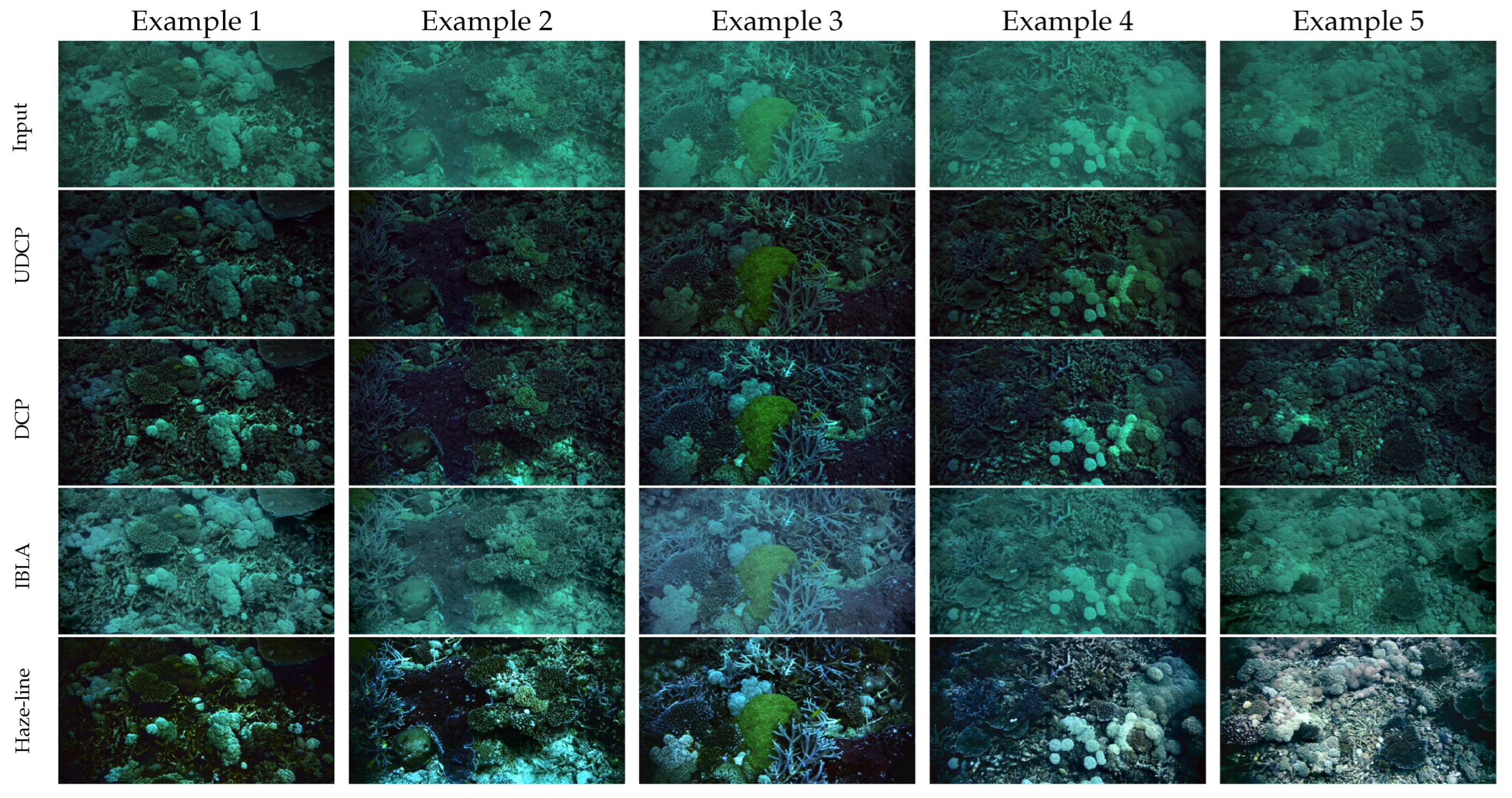
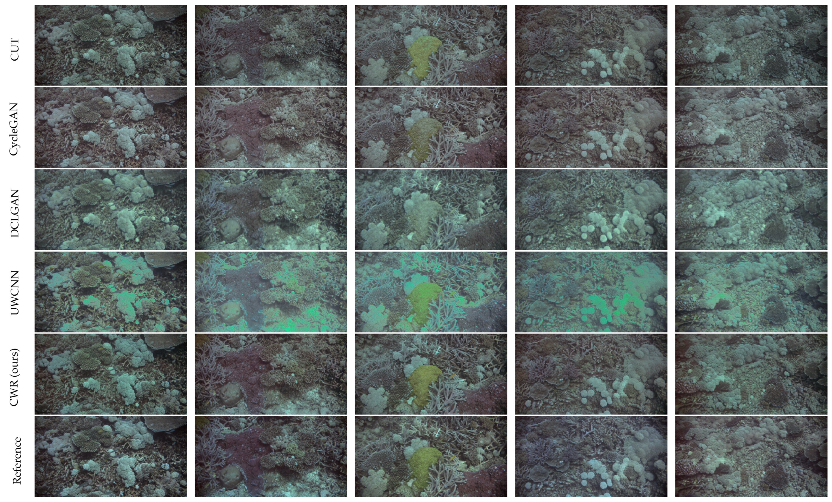
3.4. Evaluation Results

Table 3 provides a quantitative evaluation, where no method always wins in terms of all metrics. However, CWR performs better than all the baseline in full-reference metrics. CWR also shows competitive results in UIQM and FID score. This suggests that CWR performs accurate restoration, and the outputs of CWR are consistent with human visual perception. Restoration methods tend to have a lower FID score, while enhancement methods tend to have a higher UIQM score. Restoration methods provide more similar outputs to our reference restored images, while the outputs of enhancement methods are more consistent with human visual perception. This is due to the objectives of restoration and enhancement being different. Conventional restoration methods run slowly, while enhancement methods tend to run faster.
Figure 7 presents the randomly selected qualitative results. Learning-based methods provide better restoration results than conventional restoration methods, where conventional restoration methods fail to perform the correct restoration. Such a phenomenon is shown in UDCP [9], DCP [8], and Haze-line [15], where they fail to remove the green-bluish tone in underwater images. CWR performs a better restoration process than other learning-based methods in keeping with the structure and content of the restored images identical to raw images with negligible artifacts.
For underwater image enhancement methods, Figure 8 shows the qualitative results of Examples 2 and 3 with zoomed patches. Conventional enhancement methods keep the structure unchanged, but sometimes over-enhance the images, adding a bright color to the objects.

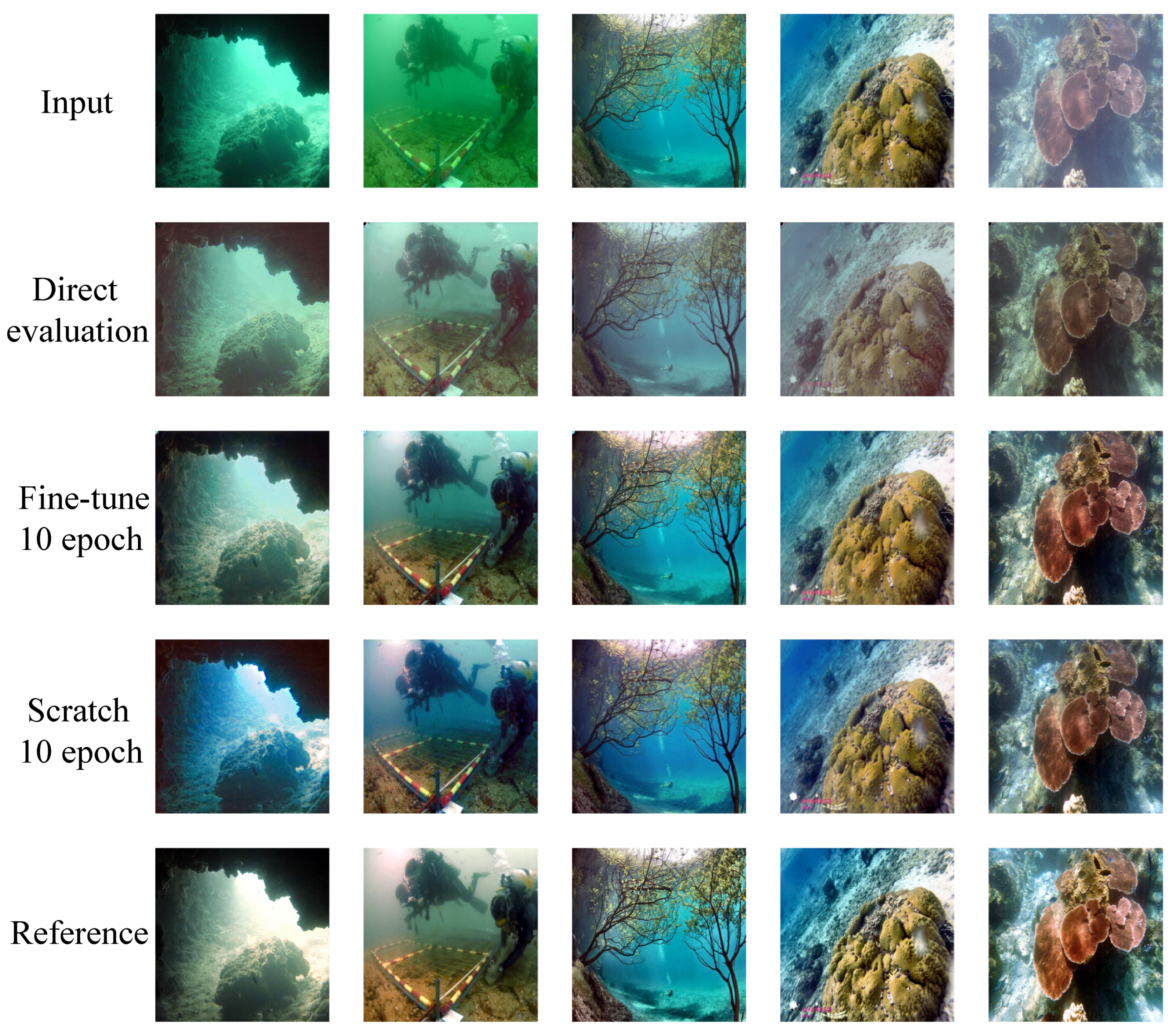
3.5. Generalization Performance on UIEB

To verify the performance of CWR, we further test it on the UIEB [25] dataset, which is an underwater image enhancement dataset containing 890 raw underwater image and enhancement image pairs. Following the data split introduced in the UIEB, we randomly choose 800 images as the training set, and train our CWR with identical settings used in the HICRD, but for 400 epochs. In test time, we used the remaining 90 images as a test set. Test images are resized to 512 × 512 resolution. Results are presented in Table 4.
We also studied the generalization of HICRD pre-trained CWR on UIEB datasets. Figure 9 shows the results of CWR on the UIEB dataset, including three cases: CWR directly evaluated on UIEB, CWR fine-tuned on UIEB for 10 epochs, and CWR trained from scratch on UIEB for 10 epochs.

3.6. Ablation Study

We conduct ablation experiments to understand the effectiveness of each component inside CWR. Table 5 presents the results.

4. Discussion

This paper described a large-scale real-world underwater restoration dataset, offering high-quality training data and proper reference restored images to support the development of both unsupervised and supervised learning-based models. Using the HICRD dataset, we evaluated recent methods from different views, including image-to-image translation approaches, conventional underwater image enhancement methods, conventional underwater image restoration methods, and learning-based restoration methods. In addition, a novel unsupervised method leveraging state-of-the-art contrastive learning techniques was proposed to fully capitalize on the HICRD dataset. In quantitative evaluations, though CWR performs better overall, there is no one method that always wins in both full-reference and non-reference metrics, suggesting new learning-based underwater image restoration methods should be developed.
Although the HICRD is a large-scale dataset, it does not cover all of the common water types. All images are acquired from Heron Island, where different sites still share similar environmental and geomorphological conditions. Most images within the HICRD are related to coral reefs. The HICRD did not capture other objects present underwater, such as shipwrecks and underwater archaeological sites [62].
We simply assume the attenuation diffuse attenuation K d and the (horizontal) attenuation coefficient β to be identical. Such an assumption is widely used in our community [15,23,63]; however, it is an incorrect assumption [6,64]. K d is an apparent optical property (AOP); it varies with sun-sensor geometry while β is an inherent optical property (IOP). This assumption leads to an imprecise restoration process; thus, an imperfect reference restored image. Moreover, following the commonly used simplified underwater imaging model consequently leads to errors. The simplified underwater imaging model ignores the absorption coefficient and ignores the difference between the backward scattering and attenuation, where attenuation is the combination of scattering and absorption. Recently, a revised underwater imaging model [6] was proposed. However, due to the complexity of this revised underwater imaging model, only a few works followed this model. More complexity leads to more parameters to estimate, where estimates inevitably contain more errors compared to accurate measurements. We do not employ the revised underwater imaging model as our imaging model to mitigate the errors from the estimation of parameters. New underwater image restoration datasets should be constructed using a more precise method, that is, employing the revised underwater imaging with fewer assumptions to generate more precise reference restored images.
The evaluation metrics for underwater image restoration are limited. Existing non-reference methods are mainly designed for underwater image enhancement; thus, if no reference restored images are provided, it would be difficult to evaluate the restoration methods. Using underwater image enhancement metrics to evaluate the restoration methods may lead to failure cases [33]. New evaluation metrics that incorporate underwater physical model properties should be developed to advance the underwater image restoration research. Furthermore, more specialized high-level task-driven evaluation metrics should be developed. Liu et al. [65] showed that the image quality assessment and detection accuracy are not strongly correlated. However, one goal of underwater image enhancement and restoration is to produce clear images to support applications in practice. Novel task-driven evaluation metrics should be developed, and they should correlate with the quality of input images.
In this paper, we focus on RGB underwater image restoration. Multi-spectral and hyper-spectral images can be used for various underwater applications [66,67,68,69]. However, few multi-spectral and hyper-spectral underwater image restoration techniques have been developed [70]. New work in underwater image restoration can consider building a benchmark dataset for multi-spectral or hyper-spectral images to further research along this critical direction.

5. Conclusions

This paper presents a real-world underwater image dataset HICRD that offers large-scale data consisting of real underwater images and restored images enabling a comprehensive evaluation of existing underwater image enhancement and restoration methods. The HICRD employs measured water parameters to create the reference restored images. We believe that the HICRD will enable a significant advancement of the use of learning-based underwater restoration methods, in both unsupervised and supervised manners. Along with the HICRD, a novel approach, CWR, employing contrastive learning, is proposed to exploit the HICRD. CWR performs a realistic underwater image restoration process in an unsupervised manner. Experimental results show that CWR performs significantly better than several conventional enhancement and restoration methods while showing more desirable results than state-of-the-art learning-based restoration methods.

Author Contributions

Conceptualization, J.H., M.S. and T.M.; methodology, J.H., M.S. and M.A.A.; code, J.H.; validation, M.S., E.B., S.A., M.A.A. and L.P.; analysis, J.H.; data collection, E.B., J.A. and R.W.; writing—original draft preparation, J.H., R.W. and E.B.; writing—review and editing, M.S., E.B., M.A.A., S.A., H.L. and L.P.; supervision, M.S., H.L. and L.P.; project administration, T.M. and L.P.; funding acquisition, T.M. and J.A. All authors have read and agreed to the published version of the manuscript.

Funding

This research was funded by Commonwealth Scientific and Industrial Research Organisation (CSIRO) through a AIM FSP_TB07_WP05: Optical sensing for marine environments project.

Data Availability Statement

The dataset presented in this study is available at GitHub: https://github.com/JunlinHan/CWR, accessed on 25 July 2022.

Acknowledgments

We thank Phillip Ford (Ocean & Atmosphere, CSIRO) for editing the manuscript. We thank the marine parks for permitting us to conduct experiments at the Great Barrier Reef (Permit G18/40267. I). We thank the anonymous reviewers for their reviews.

Conflicts of Interest

The authors declare no conflict of interest.

References

  1. Reggiannini, M.; Moroni, D. The Use of Saliency in Underwater Computer Vision: A Review. Remote Sens. 2021, 13, 22. [Google Scholar] [CrossRef]
  2. Williams, D.P.; Fakiris, E. Exploiting environmental information for improved underwater target classification in sonar imagery. IEEE Trans. Geosci. Remote Sens. 2014, 52, 6284–6297. [Google Scholar] [CrossRef]
  3. Ludeno, G.; Capozzoli, L.; Rizzo, E.; Soldovieri, F.; Catapano, I. A microwave tomography strategy for underwater imaging via ground penetrating radar. Remote Sens. 2018, 10, 1410. [Google Scholar] [CrossRef]
  4. Fei, T.; Kraus, D.; Zoubir, A.M. Contributions to automatic target recognition systems for underwater mine classification. IEEE Trans. Geosci. Remote Sens. 2014, 53, 505–518. [Google Scholar] [CrossRef]
  5. Carlevaris-Bianco, N.; Mohan, A.; Eustice, R.M. Initial results in underwater single image dehazing. In Proceedings of the Oceans 2010 Mts/IEEE Seattle, Seattle, WA, USA, 20–23 September 2010; pp. 1–8. [Google Scholar]
  6. Akkaynak, D.; Treibitz, T. A Revised Underwater Image Formation Model. In Proceedings of the IEEE Conference on Computer Vision and Pattern Recognition (CVPR), Salt Lake City, UT, USA, 18–23 June 2018; pp. 6723–6732. [Google Scholar]
  7. Yuan, J.; Cao, W.; Cai, Z.; Su, B. An Underwater Image Vision Enhancement Algorithm Based on Contour Bougie Morphology. IEEE Trans. Geosci. Remote Sens. 2020, 59, 8117–8128. [Google Scholar] [CrossRef]
  8. He, K.; Sun, J.; Tang, X. Single image haze removal using dark channel prior. IEEE Trans. Pattern Anal. Mach. Intell. 2010, 33, 2341–2353. [Google Scholar]
  9. Drews, P.; Nascimento, E.; Moraes, F.; Botelho, S.; Campos, M. Transmission estimation in underwater single images. In Proceedings of the IEEE International Conference on Computer Vision Workshops, Sydney, NSW, Australia, 2–8 December 2013; pp. 825–830. [Google Scholar]
  10. Galdran, A.; Pardo, D.; Picón, A.; Alvarez-Gila, A. Automatic red-channel underwater image restoration. J. Vis. Commun. Image Represent. 2015, 26, 132–145. [Google Scholar] [CrossRef]
  11. Chiang, J.Y.; Chen, Y.C. Underwater image enhancement by wavelength compensation and dehazing. IEEE Trans. Image Process. 2011, 21, 1756–1769. [Google Scholar] [CrossRef]
  12. Lu, H.; Li, Y.; Zhang, L.; Serikawa, S. Contrast enhancement for images in turbid water. J. Opt. Soc. Am. A 2015, 32, 886–893. [Google Scholar] [CrossRef]
  13. Peng, Y.T.; Cosman, P.C. Underwater image restoration based on image blurriness and light absorption. IEEE Trans. Image Process. 2017, 26, 1579–1594. [Google Scholar] [CrossRef]
  14. Jerlov, N.G. Marine Optics; Elsevier: Amsterdam, The Netherlands, 1976. [Google Scholar]
  15. Berman, D.; Levy, D.; Avidan, S.; Treibitz, T. Underwater single image color restoration using haze-lines and a new quantitative dataset. IEEE Trans. Pattern Anal. Mach. Intell. 2020, 43, 2822–2837. [Google Scholar] [CrossRef] [Green Version]
  16. Schechner, Y.Y.; Karpel, N. Recovery of underwater visibility and structure by polarization analysis. IEEE J. Ocean. Eng. 2005, 30, 570–587. [Google Scholar] [CrossRef]
  17. Li, X.; Hu, H.; Zhao, L.; Wang, H.; Yu, Y.; Wu, L.; Liu, T. Polarimetric image recovery method combining histogram stretching for underwater imaging. Sci. Rep. 2018, 8, 12430. [Google Scholar] [CrossRef] [PubMed]
  18. Hu, H.; Zhang, Y.; Li, X.; Lin, Y.; Cheng, Z.; Liu, T. Polarimetric underwater image recovery via deep learning. Opt. Lasers Eng. 2020, 133, 106152. [Google Scholar] [CrossRef]
  19. Cao, K.; Peng, Y.T.; Cosman, P.C. Underwater image restoration using deep networks to estimate background light and scene depth. In Proceedings of the 2018 IEEE Southwest Symposium on Image Analysis and Interpretation (SSIAI), Las Vegas, NV, USA, 8–10 April 2018; pp. 1–4. [Google Scholar]
  20. Barbosa, W.V.; Amaral, H.G.; Rocha, T.L.; Nascimento, E.R. Visual-quality-driven learning for underwater vision enhancement. In Proceedings of the 2018 25th IEEE International Conference on Image Processing (ICIP), Athens, Greece, 7–10 October 2018; pp. 3933–3937. [Google Scholar]
  21. Cai, B.; Xu, X.; Jia, K.; Qing, C.; Tao, D. Dehazenet: An end-to-end system for single image haze removal. IEEE Trans. Image Process. 2016, 25, 5187–5198. [Google Scholar] [CrossRef]
  22. Hou, M.; Liu, R.; Fan, X.; Luo, Z. Joint residual learning for underwater image enhancement. In Proceedings of the 2018 25th IEEE International Conference on Image Processing (ICIP), Athens, Greece, 7–10 October 2018; pp. 4043–4047. [Google Scholar]
  23. Li, C.; Anwar, S.; Porikli, F. Underwater scene prior inspired deep underwater image and video enhancement. Pattern Recognit. 2020, 98, 107038. [Google Scholar] [CrossRef]
  24. Huang, G.; Liu, Z.; Van Der Maaten, L.; Weinberger, K.Q. Densely connected convolutional networks. In Proceedings of the IEEE Conference on Computer Vision and Pattern Recognition, Honolulu, HI, USA, 21–26 July 2017; pp. 4700–4708. [Google Scholar]
  25. Li, C.; Guo, C.; Ren, W.; Cong, R.; Hou, J.; Kwong, S.; Tao, D. An underwater image enhancement benchmark dataset and beyond. IEEE Trans. Image Process. 2019, 29, 4376–4389. [Google Scholar] [CrossRef]
  26. Duarte, A.; Codevilla, F.; Gaya, J.D.O.; Botelho, S.S. A dataset to evaluate underwater image restoration methods. In Proceedings of the OCEANS 2016-Shanghai, Shanghai, China, 10–13 April 2016; pp. 1–6. [Google Scholar]
  27. Fabbri, C.; Islam, M.J.; Sattar, J. Enhancing underwater imagery using generative adversarial networks. In Proceedings of the 2018 IEEE International Conference on Robotics and Automation (ICRA), Brisbane, QLD, Australia, 21–25 May 2018; pp. 7159–7165. [Google Scholar]
  28. Islam, M.J.; Xia, Y.; Sattar, J. Fast underwater image enhancement for improved visual perception. IEEE Robot. Autom. Lett. 2020, 5, 3227–3234. [Google Scholar] [CrossRef]
  29. Wang, K.; Hu, Y.; Chen, J.; Wu, X.; Zhao, X.; Li, Y. Underwater image restoration based on a parallel convolutional neural network. Remote Sens. 2019, 11, 1591. [Google Scholar] [CrossRef]
  30. Li, C.; Guo, J.; Guo, C. Emerging from water: Underwater image color correction based on weakly supervised color transfer. IEEE Signal Process. Lett. 2018, 25, 323–327. [Google Scholar] [CrossRef]
  31. Silberman, N.; Derek Hoiem, P.K.; Fergus, R. Indoor Segmentation and Support Inference from RGBD Images. In Proceedings of the ECCV, Florence, Italy, 7–13 October 2012. [Google Scholar]
  32. Akkaynak, D.; Treibitz, T. Sea-Thru: A Method for Removing Water From Underwater Images. In Proceedings of the IEEE/CVF Conference on Computer Vision and Pattern Recognition (CVPR), Long Beach, CA, USA, 15–20 June 2019; pp. 1682–1691. [Google Scholar]
  33. Anwar, S.; Li, C. Diving deeper into underwater image enhancement: A survey. Signal Process. Image Commun. 2020, 89, 115978. [Google Scholar] [CrossRef]
  34. He, K.; Fan, H.; Wu, Y.; Xie, S.; Girshick, R. Momentum contrast for unsupervised visual representation learning. In Proceedings of the IEEE Conference on Computer Vision and Pattern Recognition (CVPR), Seattle, WA, USA, 13–19 June 2020; pp. 9729–9738. [Google Scholar]
  35. Chen, T.; Kornblith, S.; Norouzi, M.; Hinton, G. A simple framework for contrastive learning of visual representations. In Proceedings of the International Conference on Machine Learning (ICML), Virtual Event, 13–18 July 2020; pp. 1597–1607. [Google Scholar]
  36. Goodfellow, I.; Pouget-Abadie, J.; Mirza, M.; Xu, B.; Warde-Farley, D.; Ozair, S.; Courville, A.; Bengio, Y. Generative adversarial nets. In Proceedings of the Advances in Neural Information Processing Systems (NIPS), Montreal, QC, Canada, 8–13 December 2014; pp. 2672–2680. [Google Scholar]
  37. Han, J.; Shoeiby, M.; Malthus, T.; Botha, E.; Anstee, J.; Anwar, S.; Wei, R.; Petersson, L.; Armin, M.A. Single Underwater Image Restoration by contrastive learning. In Proceedings of the IEEE International Geoscience and Remote Sensing Symposium (IGARSS), Brussels, Belgium, 11–16 July 2021. [Google Scholar]
  38. Salmond, J.; Passenger, J.; Kovacs, E.; Roelfsema, C.; Stetner, D. Reef Check Australia 2018 Heron Island Reef Health Report; Reef Check Foundation Ltd.: Marina Del Rey, CA, USA, 2018. [Google Scholar]
  39. Schönberg, C.H.; Suwa, R. Why bioeroding sponges may be better hosts for symbiotic dinoflagellates than many corals. In Porifera Research: Biodiversity, Innovation and Sustainability; Museu Nacional: Rio de Janeiro, Brazil, 2007; pp. 569–580. [Google Scholar]
  40. Boss, E.; Twardowski, M.; McKee, D.; Cetinić, I.; Slade, W. Beam Transmission and Attenuation Coefficients: Instruments, Characterization, Field Measurements and Data Analysis Protocols, 2nd ed.; IOCCG Ocean Optics and Biogeochemistry Protocols for Satellite Ocean Colour Sensor Validation; IOCCG: Dartmouth, NS, Canada, 2019. [Google Scholar]
  41. Oubelkheir, K.; Ford, P.W.; Clementson, L.A.; Cherukuru, N.; Fry, G.; Steven, A.D.L. Impact of an extreme flood event on optical and biogeochemical properties in a subtropical coastal periurban embayment (Eastern Australia). J. Geophys. Res. Ocean. 2014, 119, 6024–6045. [Google Scholar] [CrossRef]
  42. Mannino, A.; Novak, M.G.; Nelson, N.B.; Belz, M.; Berthon, J.F.; Blough, N.V.; Boss, E.; Brichaud, A.; Chaves, J.; Del Castillo, C.; et al. Measurement Protocol of Absorption by Chromophoric Dissolved Organic Matter (CDOM) and Other Dissolved Materials, 1st ed.; IOCCG Ocean Optics and Biogeochemistry Protocols for Satellite Ocean Colour Sensor Validation; IOCCG: Dartmouth, NS, Canada, 2019. [Google Scholar]
  43. Austin, R.W.; Petzold, T.J. The Determination of the Diffuse Attenuation Coefficient of Sea Water Using the Coastal Zone Color Scanner. In Oceanography from Space; Gower, J.F.R., Ed.; Springer: Boston, MA, USA, 1981; pp. 239–256. [Google Scholar] [CrossRef]
  44. Simon, A.; Shanmugam, P. A new model for the vertical spectral diffuse attenuation coefficient of downwelling irradiance in turbid coastal waters: Validation with in situ measurements. Opt. Express 2013, 21, 30082–30106. [Google Scholar] [CrossRef] [PubMed]
  45. Panetta, K.; Gao, C.; Agaian, S. Human-visual-system-inspired underwater image quality measures. IEEE J. Ocean. Eng. 2015, 41, 541–551. [Google Scholar] [CrossRef]
  46. Mittal, A.; Soundararajan, R.; Bovik, A.C. Making a “completely blind” image quality analyzer. IEEE Signal Process. Lett. 2012, 20, 209–212. [Google Scholar] [CrossRef]
  47. Mittal, A.; Moorthy, A.K.; Bovik, A.C. No-reference image quality assessment in the spatial domain. IEEE Trans. Image Process. 2012, 21, 4695–4708. [Google Scholar] [CrossRef]
  48. Serikawa, S.; Lu, H. Underwater image dehazing using joint trilateral filter. Comput. Electr. Eng. 2014, 40, 41–50. [Google Scholar] [CrossRef]
  49. Park, T.; Efros, A.A.; Zhang, R.; Zhu, J.Y. Contrastive learning for unpaired image-to-image translation. In Proceedings of the European Conference on Computer Vision, Munich, Germany, 8–14 September; pp. 319–345.
  50. Zhu, J.Y.; Park, T.; Isola, P.; Efros, A.A. Unpaired image-to-image translation using cycle-consistent adversarial networks. In Proceedings of the IEEE International Conference on Computer Vision, Venice, Italy, 22–29 October 2017; pp. 2223–2232. [Google Scholar]
  51. Han, J.; Shoeiby, M.; Petersson, L.; Armin, M.A. Dual Contrastive Learning for Unsupervised Image-to-Image Translation. In Proceedings of the IEEE/CVF Conference on Computer Vision and Pattern Recognition Workshops, Nashville, TN, USA, 19–25 June 2021. [Google Scholar]
  52. He, K.; Zhang, X.; Ren, S.; Sun, J. Deep residual learning for image recognition. In Proceedings of the IEEE Conference on Computer Vision and Pattern Recognitio (CVPR), Las Vegas, NV, USA, 27–30 June 2016; pp. 770–778. [Google Scholar]
  53. Isola, P.; Zhu, J.Y.; Zhou, T.; Efros, A.A. Image-to-Image Translation with Conditional Adversarial Networks. In Proceedings of the IEEE Conference on Computer Vision and Pattern Recognition (CVPR), Honolulu, HI, USA, 21–26 July 2017; pp. 1125–1134. [Google Scholar]
  54. Li, C.Y.; Guo, J.C.; Cong, R.M.; Pang, Y.W.; Wang, B. Underwater image enhancement by dehazing with minimum information loss and histogram distribution prior. IEEE Trans. Image Process. 2016, 25, 5664–5677. [Google Scholar] [CrossRef]
  55. Fu, X.; Zhuang, P.; Huang, Y.; Liao, Y.; Zhang, X.P.; Ding, X. A retinex-based enhancing approach for single underwater image. In Proceedings of the International Conference on Image Processing, Paris, France, 27–30 October 2014; pp. 4572–4576. [Google Scholar]
  56. Ancuti, C.O.; Ancuti, C.; De Vleeschouwer, C.; Bekaert, P. Color balance and fusion for underwater image enhancement. IEEE Trans. Image Process. 2017, 27, 379–393. [Google Scholar] [CrossRef]
  57. Miyato, T.; Kataoka, T.; Koyama, M.; Yoshida, Y. Spectral normalization for generative adversarial networks. arXiv 2018, arXiv:1802.05957. [Google Scholar]
  58. Ulyanov, D.; Vedaldi, A.; Lempitsky, V. Instance normalization: The missing ingredient for fast stylization. arXiv 2016, arXiv:1607.08022. [Google Scholar]
  59. Kingma, D.P.; Ba, J. Adam: A method for stochastic optimization. In Proceedings of the International Conference on Learning Representations (ICLR), Banff, AB, Canada, 14–16 April 2014. [Google Scholar]
  60. Wang, Z.; Bovik, A.C.; Sheikh, H.R.; Simoncelli, E.P. Image quality assessment: From error visibility to structural similarity. IEEE Trans. Image Process. 2004, 13, 600–612. [Google Scholar] [CrossRef] [PubMed] [Green Version]
  61. Heusel, M.; Ramsauer, H.; Unterthiner, T.; Nessler, B.; Hochreiter, S. Gans trained by a two time-scale update rule converge to a local nash equilibrium. In Proceedings of the Advances in Neural Information Processing Systems, Long Beach, CA, USA, 4–9 December 2017. [Google Scholar]
  62. Mangeruga, M.; Bruno, F.; Cozza, M.; Agrafiotis, P.; Skarlatos, D. Guidelines for underwater image enhancement based on benchmarking of different methods. Remote Sens. 2018, 10, 1652. [Google Scholar] [CrossRef]
  63. Berman, D.; Treibitz, T.; Avidan, S. Diving into haze-lines: Color restoration of underwater images. In Proceedings of the British Machine Vision Conference (BMVC), London, UK, 4–7 September 2017; Volume 1. [Google Scholar]
  64. Akkaynak, D.; Treibitz, T.; Shlesinger, T.; Loya, Y.; Tamir, R.; Iluz, D. What Is the Space of Attenuation Coefficients in Underwater Computer Vision? In Proceedings of the IEEE Conference on Computer Vision and Pattern Recognition (CVPR), Honolulu, HI, USA, 21–26 July 2017; pp. 4931–4940. [Google Scholar]
  65. Liu, R.; Fan, X.; Zhu, M.; Hou, M.; Luo, Z. Real-world underwater enhancement: Challenges, benchmarks, and solutions under natural light. IEEE Trans. Circuits Syst. Video Technol. 2020, 30, 4861–4875. [Google Scholar] [CrossRef]
  66. Yi, D.H.; Gong, Z.; Jech, J.M.; Ratilal, P.; Makris, N.C. Instantaneous 3D continental-shelf scale imaging of oceanic fish by multi-spectral resonance sensing reveals group behavior during spawning migration. Remote Sens. 2018, 10, 108. [Google Scholar] [CrossRef]
  67. Fu, X.; Shang, X.; Sun, X.; Yu, H.; Song, M.; Chang, C.I. Underwater hyperspectral target detection with band selection. Remote Sens. 2020, 12, 1056. [Google Scholar] [CrossRef]
  68. Mogstad, A.A.; Johnsen, G.; Ludvigsen, M. Shallow-water habitat mapping using underwater hyperspectral imaging from an unmanned surface vehicle: A pilot study. Remote Sens. 2019, 11, 685. [Google Scholar] [CrossRef]
  69. Dumke, I.; Ludvigsen, M.; Ellefmo, S.L.; Søreide, F.; Johnsen, G.; Murton, B.J. Underwater hyperspectral imaging using a stationary platform in the Trans-Atlantic Geotraverse hydrothermal field. IEEE Trans. Geosci. Remote Sens. 2018, 57, 2947–2962. [Google Scholar] [CrossRef]
  70. Guo, Y.; Song, H.; Liu, H.; Wei, H.; Yang, P.; Zhan, S.; Wang, H.; Huang, H.; Liao, N.; Mu, Q.; et al. Model-based restoration of underwater spectral images captured with narrowband filters. Optics Express 2016, 24, 13101–13120. [Google Scholar] [CrossRef]
Figure 1. The flowchart of this paper, where rectangles denote operations, rhombus denote images, circles denote datasets, and trapezoids denote models. We show (A) Dataset construction (Section 2.1): We construct a large-scale dataset, referred to as Heron Island Coral Reef Dataset (HICRD). We collect raw data from different sites and split the raw images into low-quality and good-quality images. We restore the good-quality images with the measured water parameters. The paired HICRD contains the good-quality images, and the corresponding reference restored images, while the unpaired HICRD contains low-quality images and the reference restored images. (B) Train the models (Section 2.2 and Section 3): We mainly train the unsupervised models using the unpaired HICRD. The paired HICRD can support the training of supervised models. (C) Test the models (Section 3): We test the trained models using the same test set and measure the predicted restored images with reference restored images.
Remotesensing 14 04297 g001
Figure 2. Location of field sites during the 2018 field campaign around Heron and Wistari Reefs. Location map is modified from [39]. Background image: Sentinel-2 true color image, acquired on 14 May 2021.
Remotesensing 14 04297 g002
Figure 3. The medium transmission t c ( x ) for six different sites/water types. HICRD contains various water types, where type1, type2, type 4, type 7, and type 8 are different. The medium transmission is formulated in Equation (5).
Remotesensing 14 04297 g003aRemotesensing 14 04297 g003b
Figure 4. Example images and split of HICRD dataset. Unpaired HICRD contains low-quality images and restored images as the training set while paired HICRD uses the good-quality images and corresponding reference restored images.
Remotesensing 14 04297 g004
Figure 5. Camera sensor response for camera sensor-type CMV2000-QE which is used to collect real underwater images.
Remotesensing 14 04297 g005
Figure 6. The overall architecture and losses of CWR. CWR targets learning a mapping G : X Y , i.e., raw underwater image → restored image. We use a ResNet-based generator with nine residual blocks and defined the first half of the generator G to be encoder. We use encoder G e n c and projection head H to extract the patch-based, multi-layer features from the raw image and its translated version (generated restored image), embedding one image to a stack of features. Each layer represents a different resolution of the patches. Here, we depict one layer only for simplification. In the stack of features, given the red “query” from the generated restored image, we set up an ( N + 1 ) -way classification problem and computed the probability that a red “positive” is selected over N blue “negatives”. Such a process shows the computation of the PatchNCE loss. We send both the generated restored image and the accurate restored image to the PatchGAN discriminator for computing adversarial loss. For each image, the discriminator outputs a result metric showing the discrimination result in the patch level. Note that the patches here are different from that computing the PatchNCE loss. We omit the identity loss here.
Remotesensing 14 04297 g006
Figure 7. Qualitative results on the test set of HICRD, where all examples are randomly selected from the test set. We compare CWR to other underwater image restoration baselines. Conventional restoration methods fail to remove the green tone in underwater images. CWR shows visual satisfactory results without content and structure loss.
Remotesensing 14 04297 g007aRemotesensing 14 04297 g007b
Figure 8. Qualitative results on the test set of HICRD for underwater image enhancement methods. Examples 2 and 3 are identical to Figure 7. Enhancement methods usually produce aesthetically pleasing results, however, enhancement methods sometimes over-enhance the images, adding bright color to the stone and coral reef against the true color of the objects. The zoomed section presents the details of color and structure.
Remotesensing 14 04297 g008aRemotesensing 14 04297 g008b
Figure 9. Results of multiple CWRs on UIEB dataset. CWR trained on HICRD scales well to greenish and green-bluish images. Features learned from HICRD can be transferred to underwater image enhancement tasks.
Remotesensing 14 04297 g009
Table 1. Detailed information of the HICRD dataset. The unpaired training set contains all low-quality images and all reference restored images while the paired training set contains 1700 good-quality images and the corresponding reference restored images. The test set contains 300 good-quality images from site 5, as well as 300 corresponding reference restored images. The water parameter for Site 3 and Site 6 are not available.
Site 1Site 2Site 3Site 4Site 5Site 6Site 7Site 8
Low-quality images475345819231726117961718
Good-quality images43711511042134452677293
Reference images2516N.A.1601241N.A.457101
Water type0102N.A.0405N.A.0708
Diver 1 max depth6.85.77.38.77.26.610.79.4
Diver 2 max depth6.46.37.68.87.46.510.49.3
Table 2. A comparison between low-quality data and good-quality data in terms of three non-reference metrics.
Number of ImagesUIQM ↑NIQE ↓BRISQUE ↓
Low quality60032.804.0733.56
Good quality36733.113.9332.58
Table 3. Comparisons to baselines on the HICRD dataset on common evaluation metrics. Category shows the categories of different methods, where L denotes learning-based, R denotes restoration, C denotes conventional, and E denotes enhancement. We show five quantitative metrics for all methods and the evaluation running speed. CWR is in the first place (in red) for MSE, PNSR, and SSIM while the second place (in blue) for FID. Based on quantitative measurements, CWR produces restored images with higher quality. Speed refers to the evaluation speed per image in seconds. CWR also runs faster than all conventional restoration methods, and on par to other learning-based restoration methods. The speed of CWR with a Tesla P100 GPU is approximately 1.5 s per image while 46 s per image on an Intel(R) Core(TM) i5-6500 CPU @ 3.20GHZ.
CategoryMethodYearMSE↓PSNR↑SSIM↑UIQM↑FID↓Speed↓
CEHistogram [54]20162408.814.440.6185.2769.1510
Retinex [55]20141227.217.360.7225.4371.905
Fusion [56]20171238.617.530.7835.3358.5785
CRUDCP [9]20133159.913.310.4894.9938.0367
DCP [8]20102548.214.270.5344.4937.52168
IBLA [13]2017803.919.420.4593.6323.06141
Haze-line [15]20202305.614.690.4274.7153.67192
LRCUT [49]2020170.326.300.7965.2622.3546
CycleGAN [50]2017448.221.810.5915.2716.7446
DCLGAN [51]2021443.821.920.7354.9324.4446
UWCNN [23]2020775.820.200.7544.1833.4355
CWR (ours)2022127.226.880.8345.2518.201.5/46
Table 4. Quantitative results assessment on the UIEB dataset. All tested images are scaled to 512 × 512 resolution. CWR consistently outperforms all baselines, suggesting the superior performance and generalization of CWR. red and blue indicates best and second best results.
MethodYearMSE↓PSNR↑SSIM↑
Histogram [54]20161576.816.480.598
Retinex [55]20143587.314.770.549
Fusion [56]2017967.219.970.705
UDCP [9]20136152.110.870.444
DCP [8]20102770.815.200.639
IBLA [13]20173587.314.770.549
CUT [49]2020860.320.340.765
CWR (ours)2022660.521.070.791
Table 5. Quantitative results for ablations: (I) no adversarial loss; (II) no PatchNCE loss; (III) no identity loss; (IV) λ i d t = 1; (V) λ i d t = 20; and (VI) replace spectral norm with instance norm. The best and second best results are highlighted in red and blue.
AblationMSE↓PSNR↑SSIM↑UIQM↑FID↓
I717.119.750.4513.6036.77
II810.519.300.7364.0644.62
III229.324.720.7395.1322.12
IV217.425.280.7565.4037.02
V203.925.540.7795.4836.35
VI160.126.160.8175.1619.46
CWR127.226.880.8345.2518.20
Publisher’s Note: MDPI stays neutral with regard to jurisdictional claims in published maps and institutional affiliations.

